

A comprehensive guide to Ordinary Least Squares (OLS) regression, including mathematical derivations, matrix formulations, step-by-step examples, and Python implementation. Learn the theory behind OLS, understand the normal equations, and implement OLS from scratch using NumPy and scikit-learn.

This article is part of the free-to-read Machine Learning from Scratch
Choose your expertise level to adjust how many terms are explained. Beginners see more tooltips, experts see fewer to maintain reading flow. Hover over underlined terms for instant definitions.
Ordinary Least Squares (OLS)
Ordinary Least Squares (OLS) is the fundamental method for estimating parameters in linear regression models. Unlike more complex machine learning algorithms that require iterative optimization, OLS provides a direct, closed-form solution that we can compute exactly using matrix algebra. This makes OLS both mathematically elegant and computationally efficient, providing a foundation for understanding more advanced regression techniques.
OLS works by finding the line (or hyperplane in multiple dimensions) that minimizes the sum of squared differences between observed values and predicted values. The "least squares" name comes from this minimization of squared errors, which has both mathematical and practical advantages. When we have a dataset with features and a target variable, OLS gives us the best-fitting linear relationship according to this squared error criterion.
In simple terms, imagine we have a scatter plot of data points and want to draw a straight line through them. OLS finds the line that makes the total squared distance from all points to the line as small as possible. This line not only shows us the general trend in our data but also allows us to make predictions for new observations.
OLS vs. Linear Regression
It's important to clarify that Ordinary Least Squares (OLS) is not a type of regression model itself, but rather a method (or formula) for estimating the parameters of a linear regression model. In other words, OLS is the mathematical procedure we use to find the best-fitting line (or hyperplane) for a set of data in linear regression.
- Linear regression refers to the statistical model that describes the relationship between the dependent variable and one or more independent variables.
- OLS is the technique most commonly used to estimate the coefficients (parameters) of that model by minimizing the sum of squared errors.
So, when we talk about "OLS regression," we're really referring to linear regression models whose parameters have been estimated using the OLS method. The OLS formula provides a systematic way to find the line (or hyperplane) that best fits the data according to the least squares criterion.
Note: While OLS is the most common method for linear regression, other estimation methods exist (such as weighted least squares, generalized least squares, or maximum likelihood estimation), but OLS remains the standard approach for basic linear regression problems.
Advantages
OLS offers several advantages that make it a preferred method for linear regression. First, it provides a closed-form solution, meaning we can compute the optimal coefficients directly using a mathematical formula rather than through iterative optimization. This makes OLS computationally efficient and typically finds the global minimum of the sum of squared errors, unlike iterative methods that might get stuck in local minima.
The method is also highly interpretable, as each coefficient represents the expected change in the target variable for a one-unit increase in the corresponding feature, holding all other features constant. This linear relationship makes it easy to understand and explain the model's predictions to stakeholders. Additionally, OLS has well-established statistical properties, including being the Best Linear Unbiased Estimator (BLUE) under the Gauss-Markov assumptions, which provides theoretical guarantees about the quality of the estimates.
Finally, OLS is well-understood, with extensive theoretical foundation and practical experience accumulated over decades. This method is applicable across a wide range of applications, and it provides a useful baseline against which to compare more complex models.
Disadvantages
Despite its strengths, OLS has several important limitations that we should be aware of. The method assumes a linear relationship between features and the target variable, which may not hold in many real-world scenarios. If the true relationship is nonlinear, OLS will provide biased and potentially misleading results.
OLS is also sensitive to outliers, as the squared error penalty means that extreme values have disproportionate influence on the final model. A single outlier can significantly shift the regression line, potentially leading to poor predictions for many of our data points. Additionally, OLS assumes that features are not perfectly correlated (no multicollinearity), as this can make the matrix inversion unstable and lead to unreliable coefficient estimates.
The method also assumes that errors are normally distributed with constant variance (homoscedasticity), and that observations are independent. Violations of these assumptions can lead to biased standard errors and incorrect statistical inferences. Finally, OLS doesn't perform any feature selection, so it will use all provided features even if some are irrelevant or redundant, potentially leading to overfitting in high-dimensional settings.
Formula
The core of OLS lies in its elegant mathematical formulation. We'll break down the mathematics step by step, starting with the intuitive approach and building up to the matrix notation.
The Objective Function
OLS seeks to minimize the sum of squared errors (SSE) between observed values and predicted values:
where:
- is the observed target value for the -th data point
- is the predicted target value for the -th data point
- is the number of data points
The predicted value comes from the linear model:
where:
- is the intercept
- are the coefficients for the features
- are the feature values for the -th data point
Deriving the Normal Equations
Let's walk through, step by step, how we derive the equations that allow us to solve for the optimal coefficients in OLS regression. This process is rooted in calculus: to find the minimum of a function (in this case, the sum of squared errors), we set its derivatives with respect to each parameter to zero. These resulting equations are called the normal equations.
Step 1: Write the Sum of Squared Errors (SSE)
Recall that the OLS objective is to minimize the sum of squared errors between the observed values and the predicted values :
where
Step 2: Take Partial Derivatives with Respect to Each Coefficient
To find the values of that minimize SSE, we take the partial derivative of SSE with respect to each coefficient and set it to zero. This is because the minimum (or maximum) of a differentiable function occurs where its derivative is zero—these are known as the critical points, and for the SSE (which is a convex function in this case), setting the derivatives to zero guarantees we find the global minimum.
Step 2.1: For the Intercept :
Let's derive the process of taking the derivative of the sum of squared errors (SSE) with respect to the intercept in detail.
Recall the SSE:
where
So, explicitly, the SSE can be written as:
We want to find the value of that minimizes SSE. To do this, we take the partial derivative of SSE with respect to :
Since the sum is over , and appears in every term, we can bring the derivative inside the sum:
Let us denote the prediction error for the -th data point as:
So each term inside the sum is . The derivative of with respect to is:
By the chain rule:
But , so
Therefore,
Putting this back into the sum, we have:
Or, equivalently,
To find the minimum, we set this derivative equal to zero:
Dividing both sides by (which does not affect the equality), we get:
This equation tells us that, at the minimum, the sum of the residuals (the differences between the observed values and the predicted values) is zero.
Now, let's substitute the explicit form of back in:
Or, written out:
This is the normal equation for the intercept in OLS regression. It states that, at the optimal values of the coefficients, the sum of the residuals is zero.
Step 2.2: For Each Slope Coefficient (where ):
Now, let's derive the process of taking the partial derivative of the sum of squared errors (SSE) with respect to a generic slope coefficient (where ):
Recall the sum of squared errors:
where the predicted value for observation is:
We want to compute the partial derivative of SSE with respect to :
Let's break this down step by step:
-
Apply the linearity of differentiation (the derivative of a sum is equal to the sum of the derivatives for each term):
The derivative of a sum is the sum of the derivatives, so we can write: -
Apply the chain rule to each term:
For each , is a function of through . The chain rule gives:Since does not depend on , its derivative is zero. The derivative of with respect to is , because:
Therefore,
So, the derivative for each term is:
-
Sum over all observations:
Putting this back into the sum, we have:Or, equivalently,
-
Set the derivative to zero to find the minimum:
To find the value of that minimizes the SSE, set the derivative equal to zero:Dividing both sides by (which does not affect the equality), we get:
This equation tells us that, at the minimum, the sum of the residuals (errors) weighted by the value of feature for each observation is zero. In other words, the residuals are orthogonal (uncorrelated) to each feature in the model.
-
Substitute the explicit form of :
Recall that . Plugging this in, we get:Or, written out more explicitly:
This is the normal equation for the slope coefficient in OLS regression. It states that, at the optimal values of the coefficients, the sum of the residuals weighted by the corresponding feature values is zero for each feature. This property is fundamental to the OLS solution and ensures that the model's errors are, on average, uncorrelated with each predictor.
Step 3: The System of Equations: The Normal Equations
We now have equations (one for each coefficient, including the intercept) in unknowns:
- One equation from setting the derivative with respect to to zero
- equations from setting the derivatives with respect to each to zero
These equations are called the normal equations. Solving this system gives us the OLS estimates for all coefficients.
In summary:
For the intercept:
For each coefficient :
This system of equations forms the foundation for the matrix solution that follows, and helps explain how OLS "balances" the errors across data points and features to find the best-fitting line or hyperplane.
Matrix Formulation
The system of normal equations we derived above can be written much more compactly and powerfully using matrix notation. This not only makes the equations easier to manipulate, but also reveals the underlying structure of the OLS solution—especially when dealing with multiple features.
Let's define the key components:
- is the design matrix of shape , where is the number of observations and is the number of features. The first column of is all ones to account for the intercept term, and the remaining columns contain the values of each feature for every observation.
- is the target vector of length , containing the observed values of the dependent variable.
- is the coefficient vector of length , which includes the intercept () and one coefficient for each feature.
In matrix notation, the model is written as:
where is the vector of errors (residuals).
The Normal Equations in Matrix Form
Recall that, for each coefficient, we set the derivative of the sum of squared errors to zero. In matrix terms, this yields the normal equations:
Here's what each part means:
- is a matrix known as the Gram matrix. It summarizes the relationships (covariances) between all pairs of features, including the intercept.
- is a -dimensional vector that captures the relationship between each feature (and the intercept) and the target variable.
Solving for the OLS Coefficients
To find the vector of coefficients that minimizes the sum of squared errors, we solve the normal equations for :
Let's break down each component of this solution:
- (Gram matrix): This matrix encodes how each feature relates to every other feature (including itself). If two features are highly correlated, the corresponding off-diagonal entry will be large.
- (Inverse of Gram matrix): This step "untangles" the relationships between features, allowing us to isolate the effect of each one. The inverse exists only if the features are not perfectly collinear (i.e., no feature is an exact linear combination of others).
- (Feature-target cross-product): This vector measures how each feature (and the intercept) is associated with the target variable across all observations.
- Matrix multiplication : This operation combines all the above information to yield the set of coefficients that minimize the sum of squared errors. Each coefficient in represents the estimated effect of its corresponding feature on the target, holding all other features constant.
Matrix Notation Benefits
This matrix formulation is not just a mathematical convenience—it is the foundation for efficient computation and for extending OLS to more complex models. It allows us to:
- Solve for all coefficients at once, regardless of the number of features
- Generalize easily to multiple regression, polynomial regression, and regularized models
- Leverage powerful linear algebra libraries for fast computation, even with large datasets
The OLS closed-form solution in matrix notation is:
This formula gives us the unique set of coefficients that minimize the sum of squared errors, provided that is invertible (i.e., the features are linearly independent).
Mathematical Properties
The OLS solution is unique if is invertible (i.e., the features are not perfectly correlated), and it globally minimizes the sum of squared errors. The solution is a linear function of the target values, and, under the Gauss-Markov assumptions, provides unbiased estimates of the true coefficients.
The condition that must be invertible is crucial. This matrix is invertible when:
- The number of observations is greater than or equal to the number of features
- No feature is a perfect linear combination of other features (no multicollinearity)
- No feature is constant (all features have some variation)
When is not invertible (singular), this indicates that the features are linearly dependent. In such cases, the OLS solution is not unique, and the problem is said to be ill-conditioned. This commonly occurs when:
- You have more features than observations ()
- Features are perfectly correlated
- One feature is a linear combination of others
In practice, numerical issues can arise even when the matrix is technically invertible but has a very large condition number, leading to unstable coefficient estimates.
A high condition number means that even tiny errors in the input data or rounding errors during computation can lead to large changes in the estimated coefficients, making them unstable and unreliable. In other words, a large condition number indicates that the matrix is nearly singular, and the OLS solution may be highly sensitive to noise or numerical imprecision.
Visualizing OLS
Let's take a step back and look at OLS from a geometric perspective—it really helps make sense of why this method is so powerful. Imagine you have a scatterplot of your data points, and you're trying to draw the best-fitting straight line through them. What OLS does is find the line where the total of all the squared vertical distances (the "residuals") from each point to the line is as small as possible. Let's see exactly how this works in practice.
This geometric interpretation reveals why OLS is both mathematically elegant and practically effective. By minimizing squared errors, OLS balances the influence of all data points, ensuring that no single observation dominates the solution while still giving more weight to larger errors. You can see how the method finds the optimal balance between fitting the data and maintaining statistical robustness.
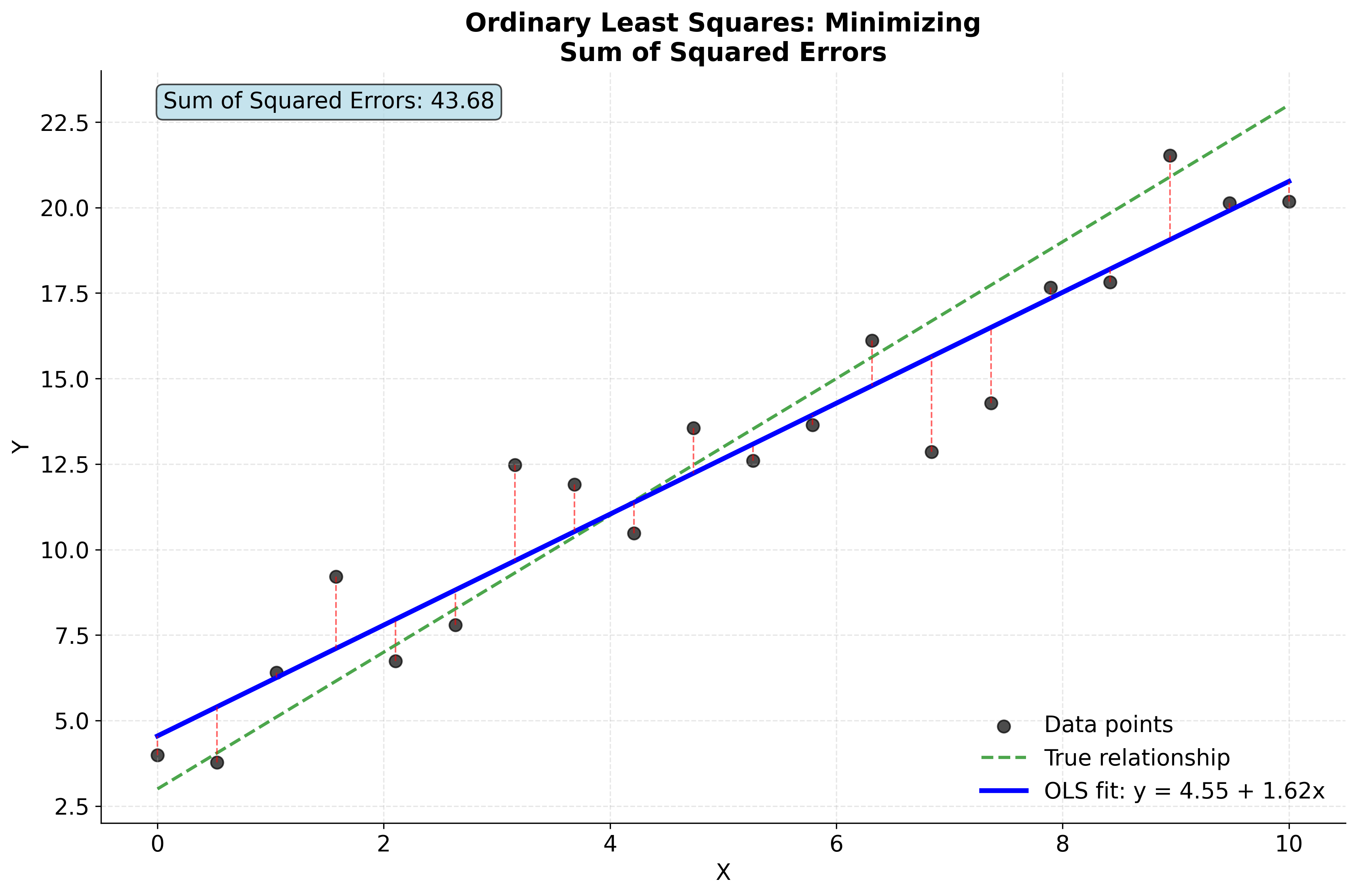
Even though the OLS fit (blue line) is very close to the true relationship (green dashed line), it does not exactly match it. This is because the observed data points contain random noise or error—real-world measurements are rarely perfect. OLS works by finding the line that minimizes the sum of squared vertical distances (residuals) between the observed data and the fitted line, not the true underlying relationship. As a result, the OLS fit represents the best possible linear approximation given the noisy data, but it will generally differ slightly from the true relationship unless there is no noise at all. This distinction highlights a fundamental aspect of statistical modeling: our estimates are always influenced by the variability and imperfections present in real data.
Example
Let's work through a step-by-step example to see exactly how the Ordinary Least Squares (OLS) solution is computed in practice. We'll use a tiny dataset so that every calculation can be shown explicitly, and you'll see how the matrix algebra connects to the underlying numbers.
Step-by-Step Calculation
Suppose we have the following dataset with four points:
| Point | ||
|---|---|---|
| 1 | 1 | 3 |
| 2 | 2 | 5 |
| 3 | 3 | 7 |
| 4 | 4 | 9 |
We want to fit a straight line of the form to this data using OLS.
Step 1: Construct the Design Matrix and Target Vector
The design matrix includes a column of ones (for the intercept) and a column for the values:
The target vector is:
Step 2: Compute
First, we take the transpose of :
Now, multiply by :
- The entry is the sum of the first column of :
- The and entries are the sum of the values:
- The entry is the sum of the squares of :
Step 3: Compute
For a matrix , the inverse is:
Plugging in our values:
- , , ,
So,
Step 4: Compute
Multiply by :
Step 5: Compute the OLS Coefficients
Now, apply the OLS formula:
Multiply the matrices:
So:
- (intercept)
- (slope)
Step 6: Interpret the Results
The OLS solution gives us the best-fitting line:
- The intercept () is
- The slope () is
This means for every unit increase in , increases by units, and when , is predicted to be .
Step 7: Verify the Fit
Let's check that this line fits all the data points exactly:
- For :
- For :
- For :
- For :
All predicted values match the observed values perfectly.
Why Does the Fit Work Perfectly Here?
In this example, the data points all lie exactly on a straight line, so OLS finds a line that passes through every point with zero error. This is an idealized case used for pedagogical purposes.
Important: In real-world data, there is usually noise, measurement error, and other sources of variation, so the OLS line will not pass through every point. Instead, it will minimize the total squared vertical distance (error) between the observed values and the predicted values. Perfect fits like this example are extremely rare in practice and may indicate overfitting or data issues.
Summary of the OLS Calculation Steps
- Build the design matrix and target vector
- Compute and
- Find the inverse
- Multiply to get
- Interpret the coefficients in the context of the problem
- (Optional) Verify predictions and fit
This step-by-step process is the foundation for all OLS regression, whether you have two points or two million. For larger datasets, the calculations are the same, but are handled by computers using efficient matrix operations. In particular, the calculation of the matrix inverse , which is required to solve for the coefficients, can be computationally intensive for very large or high-dimensional datasets. Modern numerical libraries use optimized algorithms (such as LU or Cholesky decomposition) to compute this inverse efficiently and accurately, or may use more stable techniques like solving the equivalent system of linear equations directly without explicitly forming the inverse.
Implementation
Let's implement OLS regression from scratch using NumPy to understand the underlying mathematics, then compare it with scikit-learn's implementation for practical applications.
Step 1: Generate Sample Data
First, we'll create a synthetic dataset with known relationships to test our implementation:
Step 2: Build the Design Matrix
The design matrix needs to include a column of ones for the intercept term:
The design matrix has 100 rows (observations) and 3 columns (intercept + 2 features). The first column is all ones, which allows us to estimate the intercept term in our linear model.
Step 3: Compute OLS Coefficients
Now we'll implement the OLS closed-form solution using matrix operations:
The estimated coefficients should be close to the true values, with small differences due to the random noise we added. This demonstrates that OLS is working correctly by recovering the underlying linear relationship despite the presence of noise.
Step 4: Make Predictions and Calculate Performance
Let's generate predictions and evaluate the model's performance:
The model should show good performance with a high R-squared value, meaning it explains a significant portion of the variance in the target variable. The MSE indicates the average squared prediction error, and the fitted equation shows the estimated effect of each feature on the target variable.
Step 5: Scikit-learn Implementation
For comparison, let's implement the same model using scikit-learn:
The scikit-learn implementation produces identical results to our NumPy implementation (differences are essentially zero due to numerical precision). This confirms that both methods solve the same mathematical problem, with scikit-learn providing a more robust and feature-rich interface for practical applications.
Step 6: Visualizing the Results
Let's create a visualization to see how well our OLS model fits the data:
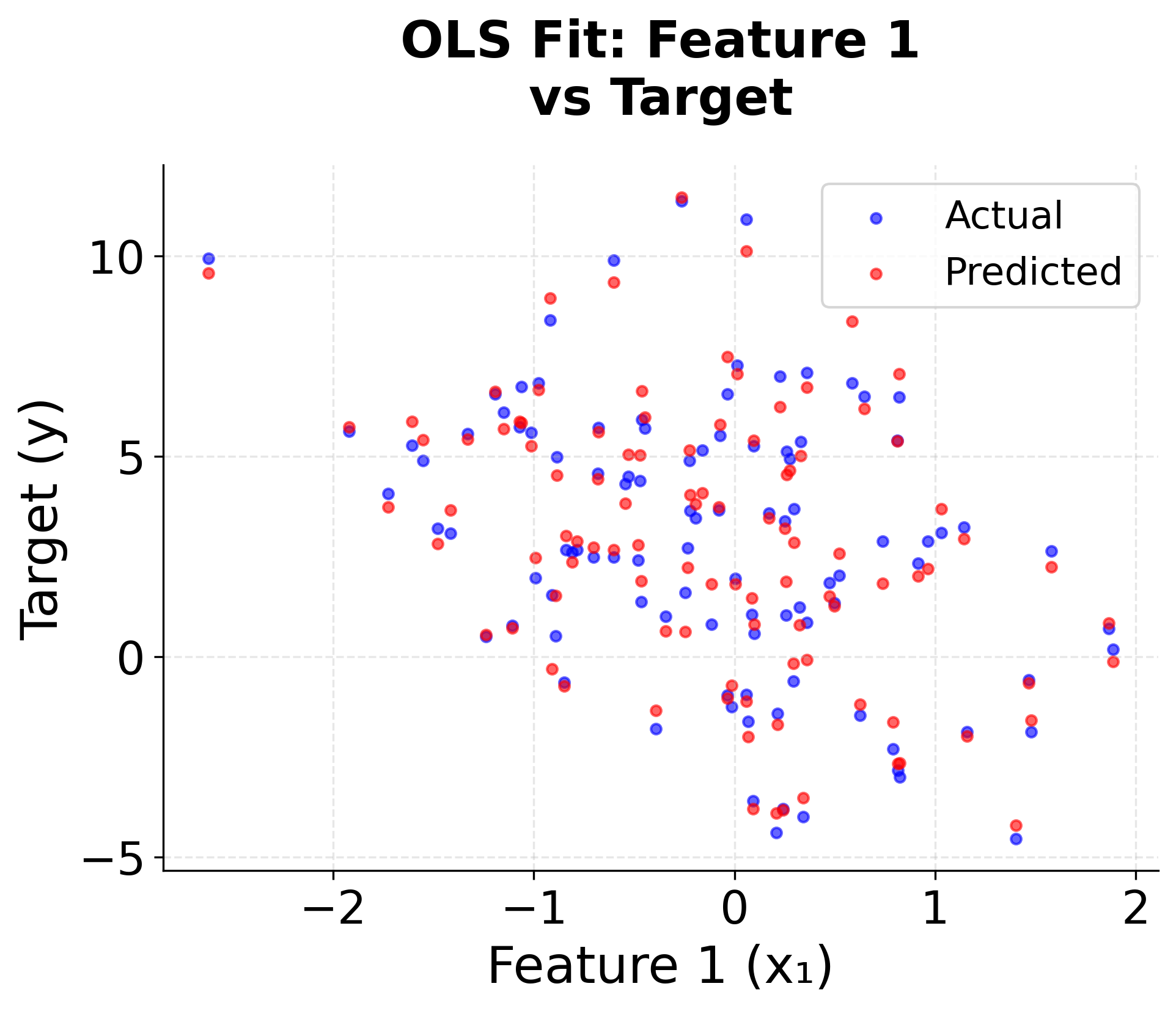
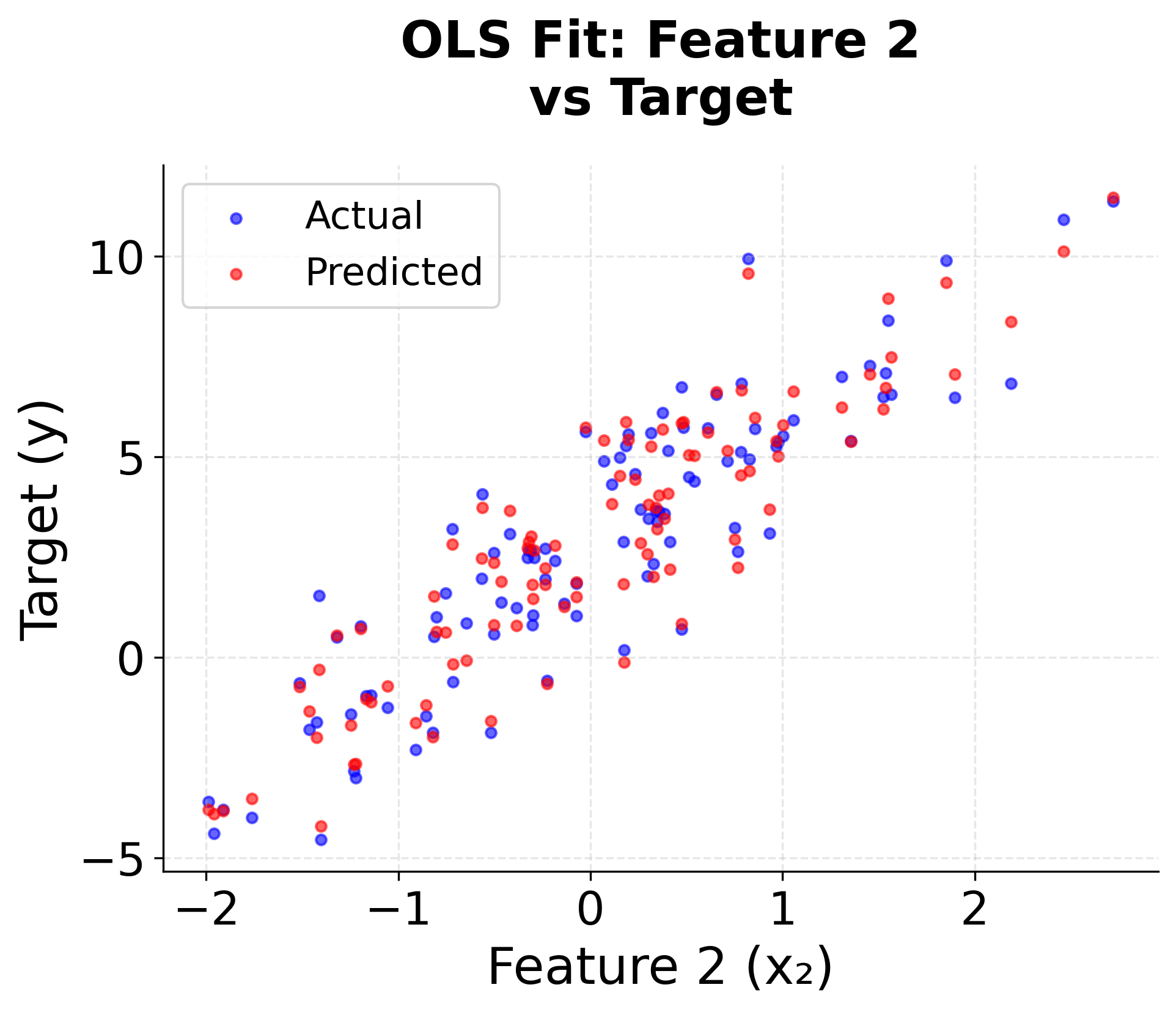
The scatter plots show how well the OLS model captures the relationships between each feature and the target variable. The close alignment between actual and predicted values (shown in blue and red respectively) confirms the model's effectiveness.
Key Parameters
Below are some of the main parameters that affect how the OLS model works and performs.
fit_intercept: Whether to calculate the intercept for this model (default: True). Set to False if you want to force the line through the origin.normalize: Whether to normalize the regressors before regression (default: False). Normalization can help with numerical stability and interpretation.copy_X: Whether to copy X or overwrite the original (default: True). Set to False to save memory for large datasets.n_jobs: Number of jobs to use for computation (default: None). Useful for parallel processing with large datasets.
Key Methods
The following are the most commonly used methods for interacting with the OLS model.
fit(X, y): Fits the linear model to the training data. X should be a 2D array of features, y should be a 1D array of target values.predict(X): Predicts target values for new data using the fitted model. Returns predicted values as a 1D array.score(X, y): Returns the coefficient of determination (R²) for the given test data and labels. Higher values indicate better fit.get_params(): Returns the parameters of the estimator. Useful for model inspection and hyperparameter tuning.
Practical Implications
OLS is most effective when there is a clear linear relationship between features and the target variable, and when interpretability is crucial for the application. The method excels in domains like economics, finance, and social sciences where understanding the magnitude and direction of relationships is as important as making accurate predictions.
Best Practices
Always examine your data for linearity assumptions before applying OLS. Use scatter plots and residual analysis to verify that relationships are approximately linear. Standardize features when they have vastly different scales to improve numerical stability and make coefficient interpretation more meaningful.
Use multiple evaluation metrics beyond just R-squared to assess model quality. Consider adjusted R-squared, AIC, BIC, and cross-validation scores. Check for multicollinearity using variance inflation factors (VIF), as highly correlated features can lead to unstable coefficient estimates. Ensure adequate sample size relative to the number of features (typically 10-15 observations per feature).
Data Requirements and Pre-processing
OLS requires features that are not perfectly correlated (no perfect multicollinearity). While OLS can handle some degree of correlation between features, extreme multicollinearity can make the matrix inversion unstable. Data standardization is often recommended when features have vastly different scales, though OLS doesn't require scaling to function.
The method assumes that errors are normally distributed with constant variance (homoscedasticity) and that observations are independent. Check these assumptions using residual analysis and statistical tests. Missing values should be handled carefully, as OLS requires complete data for all observations.
Common Pitfalls
Ignoring assumption violations, particularly linearity and homoscedasticity, can lead to biased estimates and incorrect statistical inferences. Overfitting by including too many features relative to sample size can lead to unstable coefficient estimates. Neglecting to check for outliers and influential observations is problematic, as a single extreme value can significantly affect the regression line.
Selecting features based solely on statistical significance without considering practical significance can lead to models that are statistically valid but practically meaningless. Confusing correlation with causation is a fundamental pitfall—OLS identifies statistical associations, but establishing causality requires additional evidence beyond statistical significance.
Computational Considerations
The closed-form solution can be computed efficiently using standard linear algebra operations, with computational complexity of O(p³) for matrix inversion and O(np²) for matrix multiplications. For very large datasets, consider using iterative methods or approximate solutions to avoid memory issues with storing large matrices.
The method is highly parallelizable, as matrix operations can be distributed across multiple processors. For production deployments, consider using optimized linear algebra libraries like BLAS and LAPACK for significant performance improvements.
Performance and Deployment Considerations
Use multiple evaluation criteria including R-squared, adjusted R-squared, mean squared error, and cross-validation scores to assess model quality. For statistical inference applications, pay attention to coefficient significance, confidence intervals, and residual analysis.
The interpretable nature of OLS coefficients makes it valuable for applications where model transparency is important. Each coefficient represents the expected change in the target variable for a one-unit increase in the corresponding feature, holding all other features constant.
For production deployment, OLS models are straightforward to implement and maintain. The closed-form solution means predictions can be computed quickly without iterative optimization, making the method suitable for real-time applications. Consider implementing model monitoring to detect concept drift and performance degradation over time.
Summary
Ordinary Least Squares (OLS) provides a mathematically elegant and computationally efficient method for linear regression that serves as the foundation for understanding more advanced techniques. By minimizing the sum of squared errors, OLS finds the optimal linear relationship between features and target variables, offering interpretable results and theoretical guarantees under appropriate assumptions.
The method's closed-form solution makes it computationally attractive, while its linear coefficient interpretation makes it valuable for applications requiring model transparency. However, OLS requires careful attention to its assumptions about linearity, error distribution, and feature relationships to ensure reliable results.
While OLS has limitations in handling nonlinear relationships and high-dimensional data, it remains an essential tool in the data science toolkit, particularly valuable as a baseline model and in applications where interpretability is paramount. Understanding OLS deeply provides the foundation for grasping more sophisticated regression techniques and regularization methods.
Quiz
Ready to test your understanding of Ordinary Least Squares (OLS) regression? Take this quiz to reinforce what you've learned about this fundamental parameter estimation method.

Comments