InteractiveMixed Integer Linear Programming (MILP) for Factory Optimization: Complete Guide with Mathematical Foundations & Implementation

Mixed Integer Linear Programming (MILP) for Factory Optimization

Mixed Integer Linear Programming (MILP) is a powerful optimization technique that combines the flexibility of linear programming with the discrete decision-making capabilities of integer programming. In factory optimization, MILP allows us to model complex production scenarios where we need to make discrete choices (like which machines to use, which products to produce) while optimizing continuous variables (like production quantities, resource allocation). This makes MILP particularly valuable for real-world manufacturing problems where decisions are inherently discrete but quantities are continuous.

Unlike pure linear programming, which assumes all variables can take any fractional value, MILP recognizes that many real-world decisions are binary (yes/no) or integer-valued (whole numbers of items). For example, we can't produce 2.3 machines or hire half a worker. This discrete nature makes MILP more realistic for factory optimization while maintaining the computational advantages of linear programming for the continuous aspects of the problem.

The key advantage of MILP in factory settings is its ability to handle both tactical decisions (what to produce) and strategic decisions (capacity investments, technology choices) in a single optimization framework. This integrated approach allows factory managers to optimize not just production schedules but also long-term capacity planning and resource allocation decisions.

Advantages

MILP provides several significant advantages for factory optimization. First, it offers mathematical rigor and guarantees optimal solutions (within computational limits), which is important for high-stakes manufacturing decisions where suboptimal choices can cost millions. The linear programming foundation ensures that the continuous aspects of production (quantities, resource usage) are optimized efficiently, while the integer constraints handle the discrete nature of real-world manufacturing decisions.

Second, MILP models are highly flexible and can incorporate a wide range of constraints and objectives. We can model complex relationships between products, machines, and resources, including setup costs, capacity constraints, demand requirements, and even multi-period planning horizons. This flexibility makes MILP suitable for diverse manufacturing scenarios, from simple production scheduling to complex supply chain optimization.

Third, MILP provides clear sensitivity analysis capabilities, allowing managers to understand how changes in parameters (demand, costs, capacities) affect optimal solutions. This insight is invaluable for scenario planning and risk management in manufacturing environments where conditions frequently change.

Disadvantages

Despite its power, MILP has several limitations that factory managers should consider. The most significant disadvantage is computational complexity. As the number of integer variables increases, the problem becomes exponentially harder to solve. This means that large-scale factory optimization problems may require significant computational resources and time, potentially making real-time optimization impractical for very complex scenarios.

Second, MILP requires precise mathematical modeling, which can be challenging for complex manufacturing systems. Translating real-world factory constraints into mathematical formulations requires deep understanding of both the manufacturing process and optimization theory. Poor modeling can lead to solutions that are mathematically optimal but practically infeasible.

Third, MILP assumes linear relationships between variables, which may not always reflect real-world manufacturing dynamics. While many factory optimization problems can be approximated linearly, some relationships (like economies of scale or learning curves) are inherently nonlinear and may require more complex modeling approaches or approximations.

Formula

Imagine you're managing a factory floor. Your job is to decide what to produce and how much, all while keeping costs low and staying within machine capacities. But here's the catch: some of your decisions are straightforward quantities (produce 5 units, use 12 hours), while others are all-or-nothing choices (set up the machine or don't, produce this product line or skip it). This fundamental difference between continuous quantities and discrete yes/no decisions is what makes factory optimization both challenging and interesting.

The mathematical challenge emerges because these two types of decisions interact in complex ways. You can't produce anything without first setting up the machine, but setup costs money regardless of how much you produce. Machine capacity limits how much you can make, but the capacity itself depends on which machines you've decided to set up. To solve this problem mathematically, we need a framework that can handle both continuous optimization (finding the best quantities) and discrete decision-making (choosing which setups to perform) simultaneously.

This is exactly what Mixed Integer Linear Programming provides. The "mixed" part means we combine continuous variables (for quantities) with integer or binary variables (for discrete choices). The "linear" part means all relationships are linear, making the problem computationally tractable. The "programming" part refers to optimization, finding the best solution among all possibilities.

Let's build this formulation step by step, starting with what we're trying to optimize.

Building the Objective Function: What Are We Optimizing?

Every optimization problem starts with a clear goal. In factory optimization, that goal is typically to minimize total cost. But here's where it gets interesting: manufacturing costs don't all behave the same way.

Think about what happens when you produce more units. Some costs increase proportionally: raw materials, direct labor, energy consumption. If you produce 10 units instead of 5, these costs roughly double. These are variable costs, which vary directly with production quantity.

But other costs don't change at all with quantity. Setting up a machine costs the same whether you produce 1 unit or 1000 units. Deciding to produce a product line requires the same initial investment regardless of volume. These are fixed costs, which are incurred once when you make a decision, then remain constant.

This creates a fundamental economic trade-off. If setup costs are high, you want to minimize setups, which might mean producing larger batches of fewer products. If variable costs dominate, you want to produce exactly what's needed. The optimizer needs to balance these competing forces.

To model this mathematically, we need two separate terms in our objective function:

Let's break down what each part means:

The Variable Cost Term: $\sum_{i=1}^{n} c_i x_i$

• $n$: number of products or continuous activities we can produce
• $i \in \{1, \ldots, n\}$: index running through all products
• $x_i$: how many units of product $i$ to produce (a continuous variable, $x_i \geq 0$)
• $c_i$: variable cost per unit of product $i$ (e.g., cost of materials and labor per unit)

This summation captures all costs that scale with production. If c_1 = \5$per unit and we produce$x_1 = 10$units, the cost contribution is$$5 \times 10 = $50$. The more we produce, the higher this cost becomes.

The Fixed Cost Term: $\sum_{j=1}^{m} d_j y_j$

• $m$: number of discrete setup decisions we can make
• $j \in \{1, \ldots, m\}$: index running through all setup decisions
• $y_j$: binary variable indicating whether we make setup decision $j$ ($y_j = 1$ if yes, $y_j = 0$ if no)
• $d_j$: fixed cost incurred when we make decision $j$ (setup cost)

This summation captures all costs that are triggered by discrete decisions. If d_1 = \30$and we decide to set up ($y_1 = 1$), we pay$$30$regardless of how much we produce. If we don't set up ($y_1 = 0$), we pay nothing.

Why This Structure Works

The optimizer can now make two types of decisions simultaneously:

1. Continuous decisions ($x_i$ values): How much of each product to produce
2. Discrete decisions ($y_j$ values): Which setups to perform

The objective function automatically balances these decisions. If a product has high variable costs but low setup costs, the optimizer might produce small quantities. If setup costs are high but variable costs are low, it might produce large batches to amortize the setup cost. The mathematical formulation captures this economic logic naturally.

Capturing Resource Constraints: What Limits Can We Work With?

Minimizing cost is only half the story. In the real world, we face physical and operational limits that constrain what we can actually do. Machines have finite capacity. Materials are available in limited quantities. We may have contractual obligations to meet certain demand levels. These constraints define the feasible region, the set of all production plans that are physically possible given our resources.

The mathematical challenge is that resource consumption comes from two different sources, and we need to model both:

1. Variable resource consumption from production quantities: The more we produce, the more resources we use.
2. Fixed resource consumption from setup decisions: Setting up a machine consumes resources regardless of production volume.

Modeling Variable Consumption

When we produce $x_i$ units of product $i$, we consume resources proportionally. If each unit of Product A requires 2 hours on Machine 1, then producing 5 units requires $2 \times 5 = 10$ hours. This is straightforward linear scaling.

Modeling Fixed Consumption

But discrete decisions also consume resources. Setting up Machine 1 might require 1 hour of technician time, whether we produce 1 unit or 100 units. Switching production lines might consume a fixed amount of cleaning material. These fixed consumptions happen once when we make the decision, then don't scale with production.

Combining Both Types of Consumption

For each resource $j$ (machine, material, etc.), we need to ensure that total consumption doesn't exceed available capacity $u_j$. The consumption comes from both sources, so we write:

Let's understand each component:

• $j \in \{1, \ldots, m\}$: index for each resource (Machine 1, Machine 2, Material A, etc.)
• $a_{ij}$: amount of resource $j$ consumed per unit of product $i$ (e.g., hours per unit)
• $x_i$: production quantity of product $i$ (from our objective function)
• $b_{kj}$: fixed amount of resource $j$ consumed when we make setup decision $k$
• $y_k$: binary variable for setup decision $k$ (1 if we set up, 0 if we don't)
• $u_j$: total capacity or availability of resource $j$
• $\forall j$: this constraint should hold for every resource

Why We Need Both Terms: A Concrete Example

Consider Machine 1 with 20 hours of capacity. Product A requires 2 hours per unit, and setting up for Product A requires 1 hour.

In this example:

• $x_1$: number of units of Product A to produce (continuous variable, $x_1 \geq 0$)
• $y_1$: binary variable indicating whether to set up for Product A ($y_1 = 1$ if we set up, $y_1 = 0$ if we don't)
• $a_{11} = 2$: hours of Machine 1 required per unit of Product A
• $b_{11} = 1$: fixed hours of Machine 1 required when setting up for Product A
• $u_1 = 20$: total capacity of Machine 1 in hours

The constraint for Machine 1 becomes:

Substituting the values:

Example calculation: If we decide to set up ($y_1 = 1$) and produce $x_1 = 10$ units:

• Variable consumption: $a_{11} x_1 = 2 \times 10 = 20$ hours
• Fixed consumption: $b_{11} y_1 = 1 \times 1 = 1$ hour
• Total consumption: $20 + 1 = 21$ hours

Since $21 > 20$, this violates the capacity constraint. The optimizer should either reduce production (e.g., produce 9 units: $2(9) + 1(1) = 18 + 1 = 19 \leq 20$) or skip the setup (produce 10 units without setup: $2(10) + 1(0) = 20 + 0 = 20 \leq 20$).

This dual structure, combining variable consumption from production with fixed consumption from setups, is what makes MILP constraints powerful. They capture the reality that both "how much" and "whether to" decisions consume resources.

Notational Note

You might notice that binary variables are indexed differently in the objective ($y_j$) versus constraints ($y_k$). This is a common convention: $j$ in the objective refers to setup decisions, while $j$ in constraints refers to resources. When the number of setup decisions equals the number of resources, $y_j$ and $y_k$ refer to the same variables in different contexts.

Defining Variable Types: Why Two Types Matter

The mathematical power of MILP comes from its ability to handle two fundamentally different types of variables in a single optimization problem. Understanding why we need both types, and how they differ, is crucial for grasping how MILP works.

Continuous Variables: $x_i \geq 0$

Continuous variables $x_i$ can take any non-negative real value. They represent quantities that can be measured with arbitrary precision: production volumes (3.7 units), resource allocations (12.5 hours), time durations (45.2% of capacity).

We require $x_i \geq 0$ because negative production doesn't make physical sense. You can't produce -5 units of a product. The non-negativity constraint ensures all solutions are physically meaningful.

Binary Variables: $y_k \in \{0, 1\}$

Binary variables $y_k$ are much more restrictive: they can only be 0 or 1. There's no middle ground. When $y_k = 1$, we make decision $k$ (set up the machine, produce the product line, invest in the technology). When $y_k = 0$, we don't make that decision.

This binary nature is what makes the problem "mixed integer." We're mixing continuous optimization (finding optimal quantities) with discrete decision-making (choosing which setups to perform).

Why This Constraint Is Profound

The constraint $y_k \in \{0, 1\}$ might look simple, but it has important implications. It prevents fractional setups: you cannot set up a machine "halfway" or produce a product line "75% of the way." Either you do it completely ($y_k = 1$) or you don't do it at all ($y_k = 0$).

This discrete constraint fundamentally changes the geometry of the feasible region. In pure linear programming, the feasible region is a convex polyhedron, a smooth continuous shape. But when we add integer constraints, the feasible region becomes the intersection of that polyhedron with discrete lattice points. This creates a non-convex feasible region, which is why MILP problems are computationally challenging but mathematically precise for real-world factory decisions.

The "mixed" nature means we get the best of both worlds: the efficiency of continuous optimization for quantities, combined with the precision of discrete decision-making for yes/no choices.

The Complete Formulation: Bringing It All Together

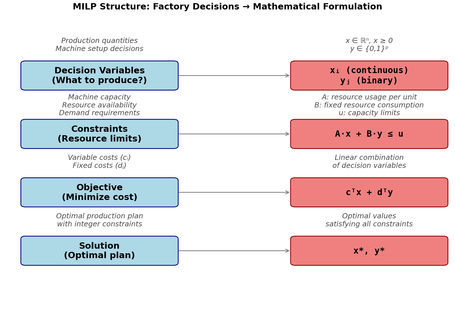
Now we can assemble the complete MILP formulation by combining the objective function with all constraints:

What This Formulation Captures

This mathematical structure captures the essence of factory optimization:

1. The objective function minimizes total cost by balancing variable costs (that scale with production) and fixed costs (that are triggered by discrete decisions).

2. The resource constraints ensure that for each resource, the total consumption from both production activities and setup decisions doesn't exceed available capacity.

3. The variable constraints ensure all solutions are physically meaningful: production quantities are non-negative, and setup decisions are binary (yes or no).

4. The optimizer's task is to find values for all $x_i$ (production quantities) and $y_k$ (setup decisions) that satisfy all constraints while achieving the minimum possible cost.

This formulation is powerful because it models the real-world interaction between continuous and discrete decisions in a mathematically precise way. The optimizer doesn't just find the best production quantities. It simultaneously determines which setups to perform, recognizing that these decisions are interdependent.

Matrix Notation: The Computational Perspective

While summation notation clearly shows the structure of the problem, computational solvers work more efficiently with matrix notation. This compact representation groups all variables and constraints into vectors and matrices, enabling efficient linear algebra operations:

Understanding the Matrix Components

• $\mathbf{x} \in \mathbb{R}^n$: vector of continuous variables (production quantities for all $n$ products), where $x_i$ is the quantity of product $i$
• $\mathbf{y} \in \{0, 1\}^p$: vector of binary variables (setup decisions for all $p$ choices), where $y_k$ indicates whether setup decision $k$ is made
• $\mathbf{c} \in \mathbb{R}^n$: vector of variable cost coefficients (cost per unit for each product), where $c_i$ is the cost per unit of product $i$
• $\mathbf{d} \in \mathbb{R}^p$: vector of fixed cost coefficients (setup cost for each decision), where $d_k$ is the fixed cost when setup decision $k$ is made
• $\mathbf{A} \in \mathbb{R}^{m \times n}$: constraint matrix mapping continuous variables to resources, where row $j$ corresponds to resource $j$ and column $i$ corresponds to product $i$. Element $A_{ji} = a_{ij}$ represents the amount of resource $j$ consumed per unit of product $i$
• $\mathbf{B} \in \mathbb{R}^{m \times p}$: constraint matrix mapping binary variables to resources, where row $j$ corresponds to resource $j$ and column $k$ corresponds to setup decision $k$. Element $B_{jk} = b_{kj}$ represents the fixed amount of resource $j$ consumed when setup decision $k$ is made
• $\mathbf{u} \in \mathbb{R}^m$: vector of resource capacities (upper bounds for all $m$ resources), where $u_j$ is the capacity of resource $j$

Why Matrix Notation Matters

The matrix form is computationally efficient because solvers can use optimized linear algebra libraries to explore the feasible region and identify optimal solutions. Matrix-vector operations are highly optimized in modern computing environments, making this representation much faster than working with individual summations.

This notation also makes problem scaling transparent: adding more products increases the size of $\mathbf{x}$ and the number of columns in $\mathbf{A}$, while adding more setup decisions increases the size of $\mathbf{y}$ and the number of columns in $\mathbf{B}$. Understanding this structure helps you anticipate how problem complexity grows with scale.

Let's visualize the structure of a MILP problem to understand how the mathematical components map to factory decisions:

Mathematical Properties: Why MILP Is Both Powerful and Challenging

Understanding the mathematical structure of MILP problems helps explain both their power and their computational challenges. The geometry of the feasible region reveals why MILP is fundamentally different from pure linear programming.

The Geometry of Feasible Regions

The feasible region of a MILP problem has a distinctive geometric structure. Imagine first the continuous relaxation, what happens if we ignore the integer constraints and allow fractional values. This creates a polyhedron: a geometric shape with flat faces, straight edges, and sharp corners. This is the feasible region of the underlying linear program.

Now impose the integer constraints. We're no longer allowed to use any point in the polyhedron, only the integer lattice points (points with integer coordinates) that lie within it. The feasible region becomes the intersection of the polyhedron with these discrete points.

This intersection creates a non-convex feasible region, which fundamentally distinguishes MILP from pure linear programming.

Why Non-Convexity Matters

In linear programming, the feasible region is convex, which guarantees that any local optimum is also a global optimum. This property enables efficient algorithms like the simplex method that can quickly find optimal solutions by moving along edges of the polyhedron.

In MILP, the non-convexity means we cannot simply follow a gradient or use simplex-like methods. We need to explore discrete points in the feasible region, which is why MILP problems are NP-hard in general. As the number of binary variables grows, the number of potential solutions grows exponentially. With $p$ binary variables, there are $2^p$ possible combinations of setup decisions to consider. This exponential growth makes exact solution increasingly difficult as problems scale.

The Silver Lining: Extreme Point Property

Despite this complexity, MILP problems have an important property that makes them solvable: if an optimal solution exists, there exists an optimal solution at an extreme point of the continuous relaxation. Extreme points are the "corners" of the polyhedron, points that can't be expressed as a convex combination of other feasible points.

This means we don't need to search through all $2^p$ possible integer combinations. We can focus our search on the corners of the feasible polyhedron where integer solutions are most likely to be found. This property is what makes branch-and-bound algorithms effective.

How Branch-and-Bound Exploits This Structure

Branch-and-bound algorithms exploit the extreme point property by solving a series of linear programming relaxations. They systematically explore extreme points while using bounds to prune away regions that cannot contain optimal solutions. The algorithm:

1. Starts with the continuous relaxation (ignoring integer constraints)
2. If the solution has fractional values, branches by fixing variables to integer values
3. Uses bounds from the LP relaxation to eliminate subproblems that can't be optimal
4. Continues until an integer solution is found and proven optimal

The Role of Duality and Bounds

Duality theory from linear programming extends to MILP through Lagrangian relaxation, where we relax some constraints and incorporate them into the objective function with penalty terms. This approach provides bounds on the optimal solution value, which helps branch-and-bound algorithms determine when they've found a solution that's close enough to optimal.

These bounds enable more efficient solution algorithms by allowing early termination when the gap between the best known solution and the best possible solution becomes sufficiently small. For large problems where exact solution is computationally infeasible, this allows us to find high-quality solutions within acceptable time limits.

Visualizing Mixed Integer Linear Programming

Let's create visualizations to understand how MILP works in practice. We'll examine a simple factory optimization problem with two products and capacity constraints.

Now let's visualize the branch-and-bound process that MILP solvers use:

Example

Let's work through a concrete factory optimization example step by step. Consider a factory that produces two products using two machines with the following specifications:

Problem Setup:

• Product 1: requires 2 hours on Machine A, 4 hours on Machine B, profit of $3 per unit
• Product 2: requires 3 hours on Machine A, 2 hours on Machine B, profit of $2 per unit
• Machine A: 12 hours available
• Machine B: 16 hours available
• Additional constraint: We can only produce products in whole units (integer constraint)

Step 1: Define Variables

Let $x_1$ = number of units of Product 1 to produce Let $x_2$ = number of units of Product 2 to produce

Step 2: Formulate the Problem

Our objective is to maximize profit: $\max 3x_1 + 2x_2$

Subject to constraints:

• Machine A capacity: $2x_1 + 3x_2 \leq 12$
• Machine B capacity: $4x_1 + 2x_2 \leq 16$
• Non-negativity: $x_1, x_2 \geq 0$
• Integer constraint: $x_1, x_2 \in \mathbb{Z}$

Step 3: Solve the LP Relaxation First

If we ignore the integer constraint, we can solve this as a linear program. We need to find where the constraint boundaries intersect, which gives us the optimal solution.

From Machine A constraint: $2x_1 + 3x_2 \leq 12$, we can express $x_2$ as:

From Machine B constraint: $4x_1 + 2x_2 \leq 16$, we can express $x_2$ as:

To find the intersection point where both constraints are binding (satisfied with equality), we set the two expressions equal:

Multiplying both sides by 3 to eliminate the denominator:

Expanding the right side:

Rearranging terms to collect $x_1$ on one side:

Simplifying:

Solving for $x_1$:

Substituting $x_1 = 3$ back into the Machine A constraint (with equality) to find $x_2$:

Simplifying:

Solving for $x_2$:

Verification: Let's verify this solution satisfies both constraints:

• Machine A: $2(3) + 3(2) = 6 + 6 = 12 \leq 12$ ✓
• Machine B: $4(3) + 2(2) = 12 + 4 = 16 \leq 16$ ✓

So the LP relaxation gives us $x_1 = 3, x_2 = 2$ with profit:

The optimal profit is \13$.

Step 4: Apply Branch-and-Bound

Since we need integer solutions, we use branch-and-bound:

Branch 1: $x_1 \leq 3$

• New constraint: $x_1 \leq 3$
• With $x_1 = 3$ fixed, from Machine A: $2(3) + 3x_2 \leq 12$, so $3x_2 \leq 12 - 6 = 6$, giving $x_2 \leq 2$
• From Machine B: $4(3) + 2x_2 \leq 16$, so $2x_2 \leq 16 - 12 = 4$, giving $x_2 \leq 2$
• The binding constraint is $x_2 \leq 2$, so the solution is $x_1 = 3, x_2 = 2$ (this is already an integer solution)
• Profit = $3(3) + 2(2) = 9 + 4 = 13$

Branch 2: $x_1 \geq 4$

• New constraint: $x_1 \geq 4$
• From Machine B: $4x_1 + 2x_2 \leq 16$, with $x_1 = 4$: $4(4) + 2x_2 \leq 16$
• Simplifying: $16 + 2x_2 \leq 16$, so $2x_2 \leq 0$, giving $x_2 \leq 0$
• Since $x_2 \geq 0$ (non-negativity), we have $x_2 = 0$
• Solution: $x_1 = 4, x_2 = 0$ (integer solution)
• Profit = $3(4) + 2(0) = 12 + 0 = 12$

Branch 1.1: $x_1 \leq 3$ and $x_2 \leq 1$

• With $x_1 = 3$ and $x_2 = 1$:
• Verification: Machine A: $2(3) + 3(1) = 6 + 3 = 9 \leq 12$ ✓
• Verification: Machine B: $4(3) + 2(1) = 12 + 2 = 14 \leq 16$ ✓
• Solution: $x_1 = 3, x_2 = 1$ (integer solution)
• Profit = $3(3) + 2(1) = 9 + 2 = 11$

Branch 1.2: $x_1 \leq 3$ and $x_2 \geq 2$

• With $x_1 = 3$ and $x_2 = 2$:
• Verification: Machine A: $2(3) + 3(2) = 6 + 6 = 12 \leq 12$ ✓
• Verification: Machine B: $4(3) + 2(2) = 12 + 4 = 16 \leq 16$ ✓
• Solution: $x_1 = 3, x_2 = 2$ (integer solution)
• Profit = $3(3) + 2(2) = 9 + 4 = 13$

Step 5: Compare Integer Solutions

We have found three feasible integer solutions:

• Solution 1: $x_1 = 3, x_2 = 1$, Profit = $3(3) + 2(1) = 9 + 2 = 11$
• Solution 2: $x_1 = 4, x_2 = 0$, Profit = $3(4) + 2(0) = 12 + 0 = 12$
• Solution 3: $x_1 = 3, x_2 = 2$, Profit = $3(3) + 2(2) = 9 + 4 = 13$

Since we're maximizing profit, the optimal integer solution is Solution 3: $x_1 = 3, x_2 = 2$ with a profit of \13$.

Note: In this example, the LP relaxation solution $(3, 2)$ happens to be an integer solution, so the integer constraint doesn't reduce the optimal value. This is not always the case. Often, integer constraints force us to accept a lower objective value than the LP relaxation.

Let's visualize this example to see the LP relaxation solution compared to the integer solutions:

Note: In this case, the LP relaxation happens to give an integer solution. However, the integer constraint ensures we only consider feasible integer points

Implementation in Google OR-Tools

Google OR-Tools provides an excellent framework for solving MILP problems with its CP-SAT solver, which is specifically designed for constraint programming and mixed integer problems. OR-Tools offers both a Python API and C++ implementation, making it accessible for data scientists while maintaining high performance.

Basic Factory Optimization

Let's start with a simple factory optimization problem that demonstrates the core MILP concepts. We'll solve the two-product problem from our earlier example using OR-Tools.

First, we set up the problem by creating a solver, defining variables, and specifying constraints:

Now let's display the results:

The solver found an optimal solution. The production quantities and profit values shown above match our earlier manual calculation. The constraint verification confirms that both machines are fully utilized, with Machine A using exactly its full capacity of 12 hours and Machine B using its full capacity of 16 hours. This full utilization indicates that the solution is efficient and that the capacity constraints are binding, meaning we cannot increase production without violating constraints. When both constraints are binding at the optimal solution, it suggests that the problem is well-formulated and that the solver has found the true optimal point where no further improvement is possible.

Advanced Factory Optimization with Setup Costs

Now let's tackle a more realistic factory optimization problem that includes setup costs and multiple products. This demonstrates how binary variables model discrete setup decisions alongside continuous production quantities.

We'll optimize production of three products across three machines, where each product requires a setup (incurring a fixed cost) before production can begin:

Let's examine the optimization results:

The optimization results demonstrate how the solver balances production quantities against setup costs. Products with higher profit margins and lower setup costs are prioritized in the optimal solution, while products that don't contribute enough to cover their setup costs may be excluded entirely. For example, if a product has a setup cost of $50 but only generates $40 in profit, the solver will set its production to zero rather than incurring a net loss.

The machine utilization percentages indicate how efficiently each machine is being used. Values near 100% suggest that machine capacity is a binding constraint, meaning that increasing capacity would allow for higher production and potentially greater profit. Lower utilization (e.g., below 80%) might indicate that other constraints, such as demand limits, setup cost trade-offs, or resource availability on other machines, are preventing full machine usage. In such cases, the bottleneck is not the machine capacity itself but rather other factors in the optimization problem.

Let's visualize the results from the advanced factory optimization:

Sensitivity Analysis

Understanding how changes in problem parameters affect optimal solutions is crucial for decision-making. Let's perform sensitivity analysis by solving the optimization problem under different scenarios: