InteractiveBoosted Trees: Complete Guide to Gradient Boosting Algorithm & Implementation

Boosted Trees

Boosted trees, also known as gradient boosting, is a powerful ensemble learning method that builds a strong predictive model by sequentially combining multiple weak learners (typically decision trees). Unlike Random Forest, which trains trees independently and combines them through voting or averaging, boosted trees train each new tree to correct the mistakes made by the previous trees in the ensemble. This sequential, error-correcting approach allows boosted trees to achieve exceptional predictive performance, often outperforming other machine learning algorithms.

The core idea behind boosted trees is to start with a simple model (often just the mean of the target variable) and then iteratively add new trees that focus on the residuals—the errors made by the current ensemble. Each new tree is trained to predict these residuals, and when added to the ensemble, it helps correct the previous mistakes. This process continues until a stopping criterion is met, resulting in a powerful ensemble that can capture complex patterns in the data.

In simple terms, boosted trees work like a student learning from their mistakes: they start with a basic understanding, identify where they went wrong, focus on correcting those specific errors, and gradually build up their knowledge through this iterative improvement process. This approach typically produces models that are highly accurate and can handle complex, non-linear relationships in the data.

Advantages

Boosted trees offer several compelling advantages that make them one of the most powerful machine learning algorithms available. First, they often achieve state-of-the-art predictive performance across a wide variety of problems, frequently outperforming other algorithms including Random Forest, neural networks, and linear models. This exceptional performance makes boosted trees particularly valuable when accuracy is the primary concern.

Additionally, boosted trees can handle both numerical and categorical features effectively without requiring extensive preprocessing, and they can automatically capture complex non-linear relationships and feature interactions without explicit feature engineering. The algorithm is also robust to outliers and can handle missing values, making it suitable for real-world datasets that often contain imperfect data.

Another significant advantage is that boosted trees provide built-in feature importance measures, allowing you to understand which features are most influential in making predictions. The algorithm also offers flexibility in the choice of loss functions, making it adaptable to different types of problems (regression, classification, ranking, etc.). Finally, boosted trees can be fine-tuned extensively through hyperparameter optimization, allowing you to achieve optimal performance for your specific problem.

Disadvantages

Despite their exceptional performance, boosted trees have some limitations that are important to consider. One of the main drawbacks is that they are prone to overfitting, especially when using too many trees or when the learning rate is too high. This requires careful tuning of hyperparameters and often necessitates early stopping or other regularization techniques to prevent the model from memorizing the training data.

Another limitation is that boosted trees can be computationally expensive to train, especially when using many trees or when dealing with large datasets. The sequential nature of the algorithm means that trees cannot be trained in parallel (unlike Random Forest), which can make training time significantly longer for large models.

Boosted trees are also sensitive to noisy data and outliers, which can cause the algorithm to focus too much on correcting errors that may not be representative of the true underlying pattern. This sensitivity can lead to poor generalization performance if not properly managed through regularization or data cleaning.

Additionally, while boosted trees provide feature importance measures, the individual trees in the ensemble are not easily interpretable, and the sequential nature of the algorithm makes it difficult to understand the exact decision-making process. The models can also be quite large and memory-intensive, especially when using many trees, which can impact deployment and inference speed in production environments.

Formula

The mathematical foundation of boosted trees involves understanding how the algorithm sequentially builds an ensemble by minimizing a loss function through gradient descent. Let's break this down step by step, starting with the basic structure and progressing to the complete algorithm formulation.

The Ensemble Model

The final boosted tree model is an ensemble of $M$ decision trees, where each tree is trained sequentially to correct the errors of the previous trees. The prediction for a given input $\mathbf{x}$ is:

$\hat{y} = \sum_{m=1}^{M} \gamma_m h_m(\mathbf{x})$

where:

• $\hat{y}$ is the final prediction
• $M$ is the total number of trees in the ensemble
• $\gamma_m$ is the learning rate (step size) for tree $m$
• $h_m(\mathbf{x})$ is the prediction from the $m$-th tree for input $\mathbf{x}$

The Loss Function

Boosted trees minimize a loss function $L(y, \hat{y})$ that measures how well the model's predictions match the true values. Common loss functions include:

For Regression (Mean Squared Error):

We've already covered these loss functions in previous chapters, so we are keeping the explanation brief.

The most common loss function for regression tasks in gradient boosting is the Mean Squared Error (MSE). It measures the average squared difference between the actual target value $y$ and the predicted value $\hat{y}$:

$L(y, \hat{y}) = \frac{1}{2}(y - \hat{y})^2$

The factor of $\frac{1}{2}$ is included for mathematical convenience because when you take the derivative of $\frac{1}{2}(y - \hat{y})^2$ with respect to $\hat{y}$, the 2 from the exponent cancels with the $\frac{1}{2}$, leaving just $(\hat{y} - y)$; this makes the gradient expression simpler and avoids carrying an extra constant through the calculations.

During training, the algorithm tries to minimize this loss by adjusting the model so that predictions $\hat{y}$ get as close as possible to the true values $y$. The gradient of this loss with respect to $\hat{y}$ is simply $(\hat{y} - y)$, which means each new tree in the ensemble is trained to predict the residuals (errors) of the current model.

For Classification (Logistic Loss):

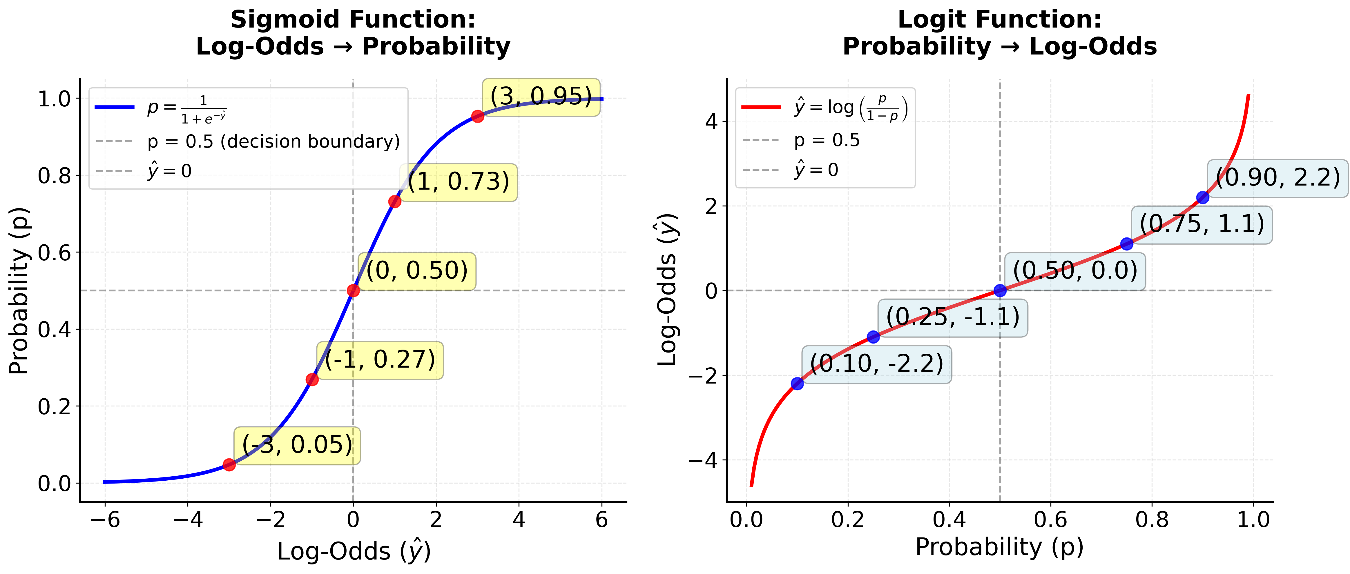
For binary classification problems, gradient boosting typically uses the logistic loss (also called log-loss or binary cross-entropy). This loss is specifically designed for situations where the target $y$ is 0 or 1, and the model's output $\hat{y}$ is a real number (not a probability, but a "logit" or "log-odds" score).

The logistic loss for a single data point is:

In gradient boosting, the logistic loss is central to the entire training process. At each boosting iteration (i.e., for each new tree that is added to the ensemble), the algorithm evaluates the logistic loss for every training example using the current prediction $\hat{y}$ (which is the sum of the outputs from all previous trees).

The gradients of this loss with respect to $\hat{y}$ are then computed for each example, and the next tree is trained to predict these gradients (also called "pseudo-residuals"). This means that the logistic loss is used repeatedly, at every boosting step and for every data point, to guide the model's updates and help it focus on the examples that are currently hardest to classify.

Let's look at how this loss function connects to log-odds and probabilities, step by step.

1. Model Output ($\hat{y}$):
   In gradient boosting for classification, the model does not directly output a probability. Instead, it outputs a real number $\hat{y}$ for each example. This number is called the logit or log-odds.

2. From Log-Odds to Probability:
   To get a probability $p$ from $\hat{y}$, we use the sigmoid (logistic) function:

   $$p = \frac{1}{1 + e^{-\hat{y}}}$$

   This maps any real value to a number between 0 and 1.

3. From Probability to Log-Odds:
   If you start with a probability $p$, you can get back to the log-odds (the value the model outputs) by inverting the sigmoid:

   $$\hat{y} = \log\left(\frac{p}{1-p}\right)$$

   So, the model is really building up an estimate of the log-odds for each example.

1. Why does the loss use $\hat{y}$ and not $p$?
   You might notice that the loss function is expressed in terms of $\hat{y}$ (the log-odds), while the sigmoid function uses $p$ (the probability). This is intentional: the model predicts and updates values in the log-odds space, not directly in probability space.

   This is because the logistic loss is derived from the negative log-likelihood of the Bernoulli distribution. Let's walk through the full derivation:

   1. Start with the Bernoulli likelihood:
      First, we write down the likelihood function for a single data point, which gives the probability of observing $y \in \{0, 1\}$ given the predicted probability $p$.

      $$P(y|p) = p^y (1-p)^{1-y}$$

   2. Take the negative log-likelihood:
      Next, we take the negative logarithm of the likelihood to obtain the loss function that we want to minimize.

      $$-\log P(y|p) = -\log\left(p^y (1-p)^{1-y}\right) = -y \log p - (1-y) \log (1-p)$$

   3. Express $p$ in terms of the model output $\hat{y}$:
      Then, we rewrite the probability $p$ in terms of the model's output $\hat{y}$ (the log-odds), since this is what the model actually predicts.

      $$p = \frac{1}{1 + e^{-\hat{y}}}$$

      and

      $$1 - p = \frac{e^{-\hat{y}}}{1 + e^{-\hat{y}}}$$

   4. Substitute $p$ and $1-p$ into the loss:
      Now, we substitute the expressions for $p$ and $1-p$ in terms of $\hat{y}$ back into the loss function.

      $$-y \log p - (1-y) \log (1-p) = -y \log\left(\frac{1}{1 + e^{-\hat{y}}}\right) - (1-y) \log\left(\frac{e^{-\hat{y}}}{1 + e^{-\hat{y}}}\right)$$

   5. Simplify the expression:
      Finally, we simplify the resulting expression to obtain the standard form of the logistic loss in terms of $\hat{y}$.

      $$= -y \left[ -\log(1 + e^{-\hat{y}}) \right] - (1-y) \left[ -\hat{y} - \log(1 + e^{-\hat{y}}) \right]$$ $$= y \log(1 + e^{-\hat{y}}) + (1-y) \left[ \hat{y} + \log(1 + e^{-\hat{y}}) \right]$$ $$= y \log(1 + e^{-\hat{y}}) + (1-y)\hat{y} + (1-y)\log(1 + e^{-\hat{y}})$$ $$= \log(1 + e^{-\hat{y}}) + (1-y)\hat{y}$$

      Alternatively, you may see the loss written as:

      $$L(y, \hat{y}) = y \log(1 + e^{-\hat{y}}) + (1-y) \log(1 + e^{\hat{y}})$$

      which is algebraically equivalent.

   This full derivation shows how the logistic loss arises naturally from the probabilistic model, and why it is expressed in terms of $\hat{y}$. This formulation is preferred because it simplifies the optimization process and makes the gradients easy to compute, which is essential for efficient training.

To recap, the logistic loss is derived from the negative log-likelihood of the Bernoulli distribution, and is expressed in terms of $\hat{y}$ (the log-odds) because that's what the model is actually predicting and updating at each boosting step.

Gradients and Pseudo-Residuals

The boosting algorithm computes the gradient of the loss with respect to $\hat{y}$ (where $\hat{y}$ is the log-odds score for the model's prediction, or the raw score output by the model for a given input $\mathbf{x}$) for each training example. For logistic loss, this gradient is:

This means that the "pseudo-residuals" (the targets for the next tree) are simply the difference between the true label and the current predicted probability.

• If the model predicts $p$ close to $y$ (e.g., $p=0.9$ and $y=1$), the gradient is small, so the next tree makes only a small correction.
• If the model predicts $p$ far from $y$ (e.g., $p=0.1$ and $y=1$), the gradient is large, so the next tree tries to make a bigger correction.

This process is repeated, with each new tree focusing on the mistakes of the current model, gradually improving the fit.

Log-loss has several important properties that make it well-suited for classification tasks in gradient boosting. First, it is a strictly proper scoring rule, which means it encourages the model to produce well-calibrated probability estimates. Additionally, log-loss is differentiable, a crucial feature that allows gradient-based optimization methods to be applied effectively. Another key aspect is that log-loss imposes a strong penalty on predictions that are both confident and incorrect, discouraging the model from making overconfident mistakes.

In gradient boosting for classification, the logistic loss provides a principled way to measure prediction error and guide the model's updates. At each step, the model fits a new tree to the difference between the true label and the current predicted probability, steadily reducing the overall loss and improving classification accuracy.

The Gradient Boosting Algorithm

The key insight of gradient boosting is to use the gradient of the loss function to guide the training of each new tree. Here's how it works:

Step 1: Initialize the model
Start with a simple model, typically the mean of the target variable for regression or the log-odds for classification:

• Here, $F_0(\mathbf{x})$ is the initial prediction for all inputs $\mathbf{x}$.
• $L(y_i, \gamma)$ is the loss function, measuring the error between the true value $y_i$ and a constant prediction $\gamma$.
• $n$ is the number of training examples.
• $\arg\min_{\gamma}$ means we choose the value of $\gamma$ that minimizes the total loss over all training examples.

For regression with mean squared error (MSE) loss, this simplifies to:

That is, the initial prediction is just the average of the target values.

Step 2: For each iteration $m = 1, 2, \ldots, M$:

• $m$ is the index of the current boosting iteration (tree), and $M$ is the total number of boosting rounds (trees).

2a. Calculate the negative gradient (pseudo-residuals)
For each training example $i$, calculate the negative gradient of the loss function with respect to the current model's prediction:

• $r_{im}$ is the pseudo-residual for example $i$ at iteration $m$.
• $F_{m-1}(\mathbf{x}_i)$ is the prediction for example $i$ from the previous iteration.
• The negative gradient tells us how to adjust our prediction to reduce the loss.

This gives us the "pseudo-residuals" that tell us in which direction and by how much we need to adjust our predictions.

2b. Train a new tree on the pseudo-residuals
Train a decision tree $h_m(\mathbf{x})$ to predict the pseudo-residuals:

• $h_m(\mathbf{x})$ is the new tree fitted at iteration $m$.
• The tree is trained to predict $r_{im}$ from the input features $\mathbf{x}_i$.
• The sum of squared differences means we fit the tree to the pseudo-residuals using least squares.

2c. Find the optimal step size
For each leaf $j$ in the new tree, find the optimal step size that minimizes the loss:

• $\gamma_{jm}$ is the optimal value to add to the prediction for all examples in leaf $j$ of tree $m$.
• $R_{jm}$ is the set of training examples that fall into leaf $j$ of tree $m$.
• This step ensures that each leaf's output is chosen to minimize the loss for the examples it contains.

2d. Update the model
Add the new tree to the ensemble:

• $F_m(\mathbf{x})$ is the updated prediction after adding the $m$-th tree.
• $\gamma_m$ is the step size (sometimes called the learning rate or shrinkage parameter) for this iteration. In some implementations, each leaf has its own $\gamma_{jm}$, and the update is performed leaf-wise.
• $h_m(\mathbf{x})$ is the prediction of the new tree.

Mathematical Properties

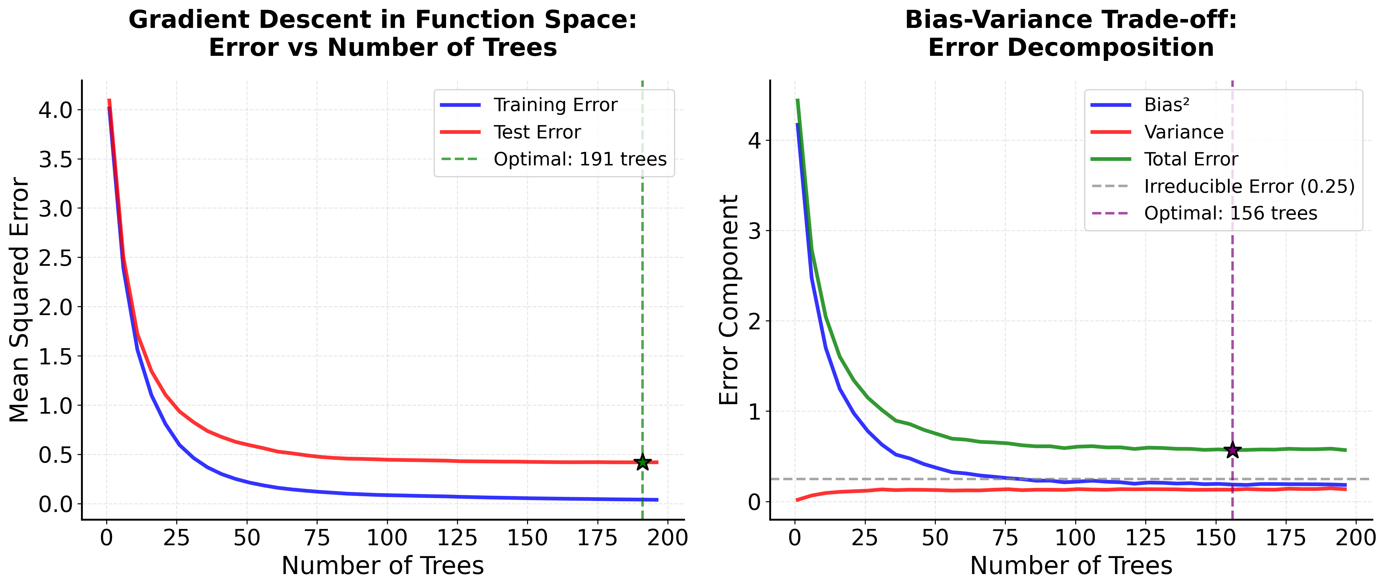
Boosted trees possess several key mathematical properties that help explain their effectiveness. One of the most important is the connection to gradient descent optimization. The algorithm can be viewed as performing gradient descent in function space, where each tree represents a step in the direction of steepest descent of the loss function.

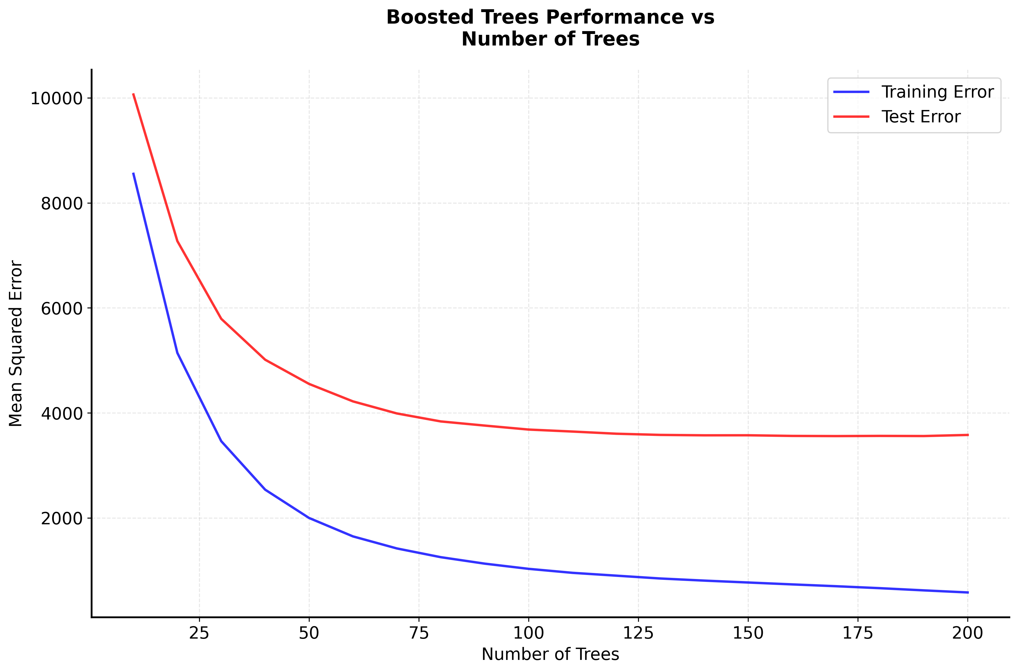
The bias-variance decomposition also applies to boosted trees, but in a different way than Random Forest. Early in the training process, the model has high bias (underfitting) but low variance. As more trees are added, the bias decreases but variance increases. The optimal number of trees balances this trade-off to minimize the total error.

Another important property is the concept of shrinkage, controlled by the learning rate $\gamma$. A smaller learning rate means smaller steps in the optimization process, which can lead to better generalization but requires more trees to achieve the same level of performance. This is often expressed as:

$\hat{y} = \sum_{m=1}^{M} \nu h_m(\mathbf{x})$

where $\nu$ is the shrinkage parameter (typically between 0.01 and 0.1) that controls the learning rate.

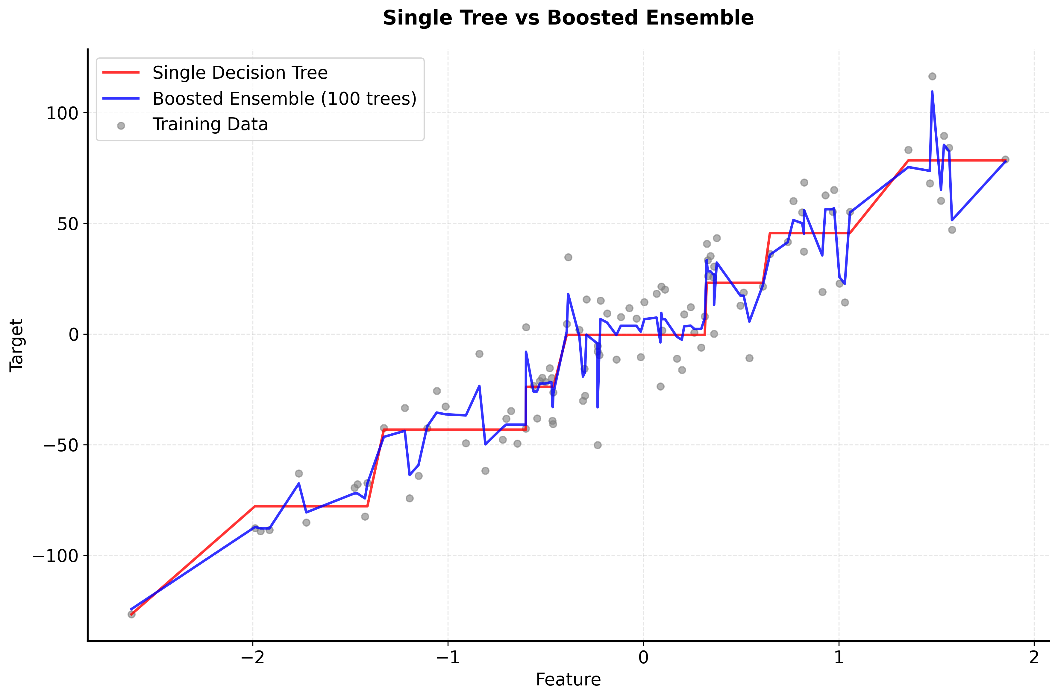
Visualizing Boosted Trees

Let's create visualizations that demonstrate how boosted trees work and how they differ from other ensemble methods.

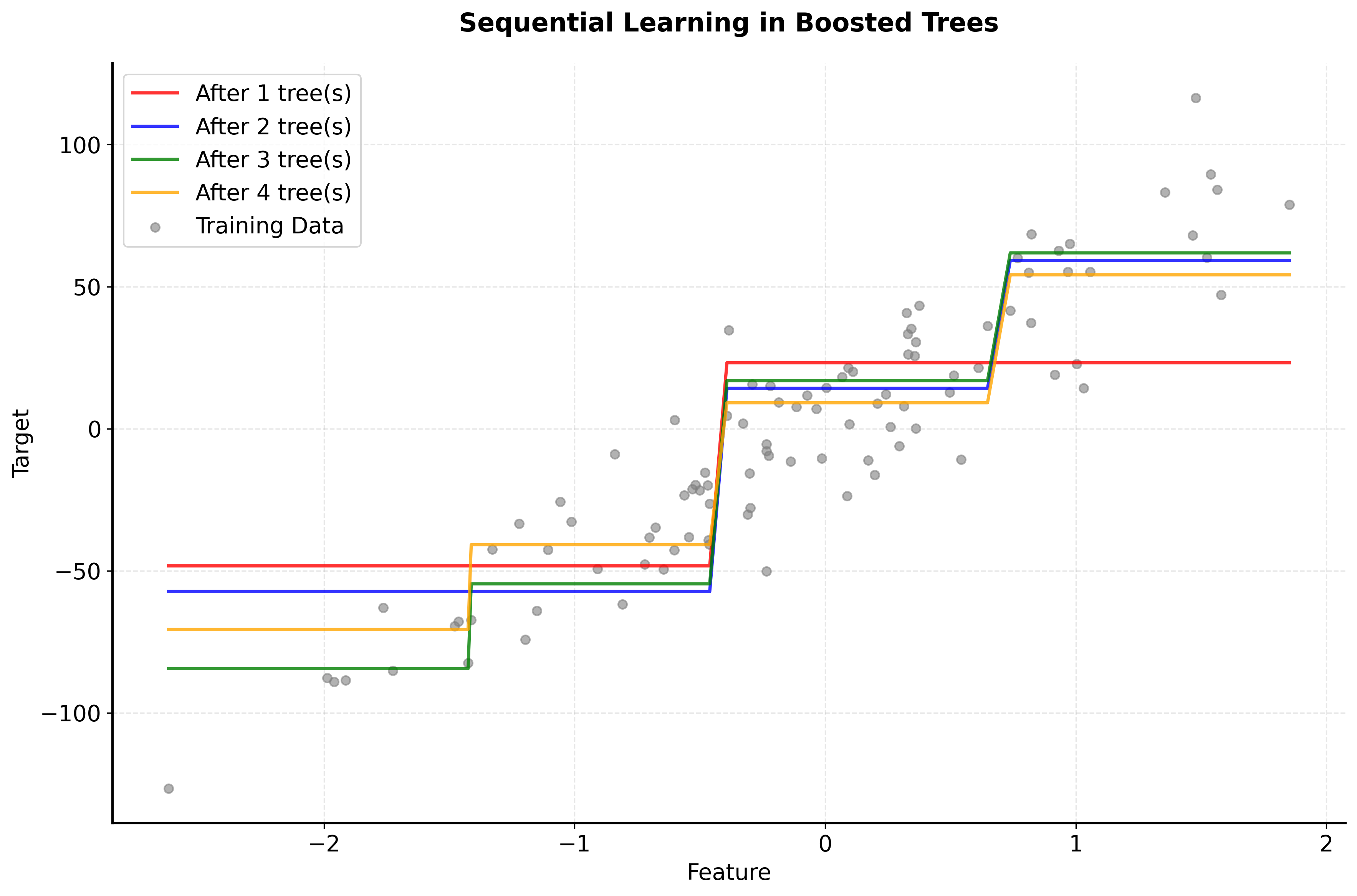
Now let's visualize how the number of trees and learning rate affect the boosting performance:

Example

Let's work through a detailed step-by-step example of boosted trees using a simple regression dataset. Suppose we want to predict house prices based on house size and number of bedrooms.

Given Data:

We have a small dataset of houses, each described by its size (in square feet), number of bedrooms, and price (in thousands):

• House Size (sq ft): [1200, 1500, 1800, 2000, 2200, 2500, 2800, 3000]
• Bedrooms: [2, 3, 3, 4, 4, 4, 5, 5]
• House Price (thousands): [180, 220, 260, 300, 340, 380, 420, 460]

Step 1: Initialize the model

The first step in gradient boosting is to start with a simple model. For regression, this is typically just the mean of the target variable. This initial prediction serves as our baseline before any trees are added.

$F_0(\mathbf{x}) = \frac{1}{8} \sum_{i=1}^{8} y_i = \frac{180 + 220 + 260 + 300 + 340 + 380 + 420 + 460}{8} = 320$

So, at this point, our model predicts 320 for every house, regardless of its features.

Step 2: Calculate pseudo-residuals for the first tree

Next, we measure how well our initial model is doing by calculating the errors (residuals) for each data point. In gradient boosting, these are called "pseudo-residuals" and, for mean squared error (MSE) loss, they are simply the difference between the true value and the current prediction.

$r_{i1} = y_i - F_0(\mathbf{x}_i) = y_i - 320$

Calculating these for each house:

• House 1: 180 - 320 = -140
• House 2: 220 - 320 = -100
• House 3: 260 - 320 = -60
• House 4: 300 - 320 = -20
• House 5: 340 - 320 = 20
• House 6: 380 - 320 = 60
• House 7: 420 - 320 = 100
• House 8: 460 - 320 = 140

These residuals represent the errors our current model makes, and the next tree will try to predict these errors.

Step 3: Train the first tree on pseudo-residuals

We now fit a decision tree to these pseudo-residuals. The tree tries to find patterns in the features (house size and bedrooms) that explain the errors made by the initial model. For simplicity, suppose the tree splits the data as follows:

• If House Size ≤ 2000: predict -80
• If House Size > 2000: predict 80

This means the tree has learned that smaller houses tend to be under-predicted (so it adds a negative correction), and larger houses are over-predicted (so it adds a positive correction).

Step 4: Find optimal step size

For each leaf of the tree, we determine how much to move the prediction in the direction suggested by the tree. This is done by finding the step size (also called the "shrinkage" or "learning rate") that minimizes the loss for the data points in that leaf. For the left leaf (House Size ≤ 2000):

$\gamma_{11} = \arg\min_{\gamma} \sum_{i: \text{size}_i \leq 2000} (y_i - (320 + \gamma \cdot (-80)))^2$

This optimization finds the best value of $\gamma$ to reduce the error for the houses in this group. The same process is repeated for the right leaf.

Step 5: Update the model

We update our model by adding the predictions from the first tree, scaled by the optimal step size:

$F_1(\mathbf{x}) = F_0(\mathbf{x}) + \gamma_1 h_1(\mathbf{x}) = 320 + \gamma_1 h_1(\mathbf{x})$

Here, $h_1(\mathbf{x})$ is the prediction from the first tree for input $\mathbf{x}$, and $\gamma_1$ is the step size we just computed.

Step 6: Calculate new pseudo-residuals

With the updated model, we again compute the pseudo-residuals, which now reflect the errors remaining after the first tree's corrections:

$r_{i2} = y_i - F_1(\mathbf{x}_i)$

These new residuals are typically smaller in magnitude, as the model has improved.

Step 7: Repeat the process

We repeat steps 3–6 for each subsequent tree. Each new tree is trained to predict the current residuals (errors), and the model is updated accordingly. Over time, the ensemble of trees becomes better at capturing the patterns in the data, as each tree focuses on the mistakes of the previous ones.

Final Prediction:

After training $M$ trees, the final prediction for a new data point is the sum of the initial prediction and the contributions from all the trees:

$\hat{y} = F_0(\mathbf{x}) + \sum_{m=1}^{M} \gamma_m h_m(\mathbf{x}) = 320 + \sum_{m=1}^{M} \gamma_m h_m(\mathbf{x})$

In summary, this example illustrates how boosted trees work: starting from a simple model, they iteratively add trees that correct the errors of the current ensemble, gradually building a more accurate predictor by focusing on the hardest-to-predict cases at each step.

Implementation in Scikit-learn

Boosted trees are implemented in scikit-learn through the GradientBoostingClassifier and GradientBoostingRegressor classes. Let's implement a complete example with proper preprocessing and evaluation:

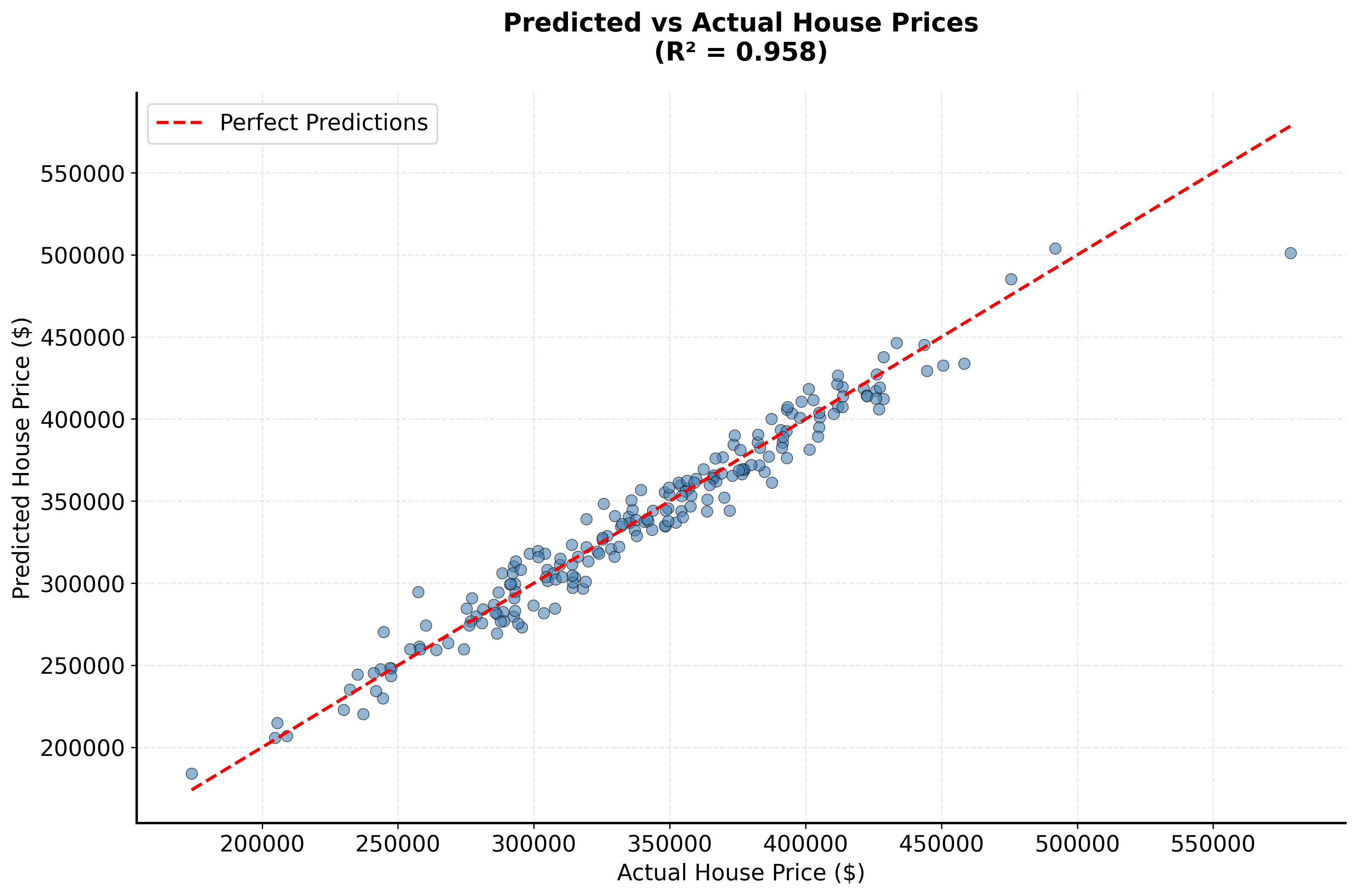
Now let's implement a regression example:

Hyperparameter Tuning

Boosted trees have several important hyperparameters that can significantly affect performance:

Key Parameters

Below are some of the main parameters that affect how Gradient Boosting works and performs.

• n_estimators: Number of boosting stages (trees) to perform (default: 100). More trees generally improve performance but increase computation time and risk of overfitting. Start with 100 and increase if validation scores improve.
• learning_rate: Shrinkage parameter that controls the contribution of each tree (default: 0.1). Lower values (0.01-0.1) require more trees but often lead to better generalization. Values between 0.01 and 0.2 work well for most datasets.
• max_depth: Maximum depth of each tree (default: 3). Controls the complexity of individual trees. Shallow trees (3-5) work well for boosting as they focus on learning simple patterns iteratively.
• min_samples_split: Minimum samples required to split an internal node (default: 2). Higher values prevent overfitting by requiring more data for splits. Values of 5-10 are commonly used.
• min_samples_leaf: Minimum samples required in a leaf node (default: 1). Higher values smooth the model and prevent overfitting. Values of 2-4 work well for most problems.
• subsample: Fraction of samples to use for fitting each tree (default: 1.0). Values less than 1.0 introduce stochastic gradient boosting, which can help prevent overfitting. Try values between 0.5 and 0.8.
• loss: Loss function to optimize (default: 'log_loss' for classification, 'squared_error' for regression). Different loss functions are appropriate for different problem types.
• random_state: Seed for reproducibility (default: None). Set to an integer to ensure consistent results across runs.

Key Methods

The following are the most commonly used methods for interacting with Gradient Boosting models.

• fit(X, y): Trains the gradient boosting model on the training data X and target values y. Each tree is trained sequentially to correct the errors of previous trees.
• predict(X): Returns predicted class labels (classification) or values (regression) for input data X by summing predictions from all trees in the ensemble.
• predict_proba(X): Returns probability estimates for each class (classification only). Useful for setting custom decision thresholds or understanding prediction confidence.
• score(X, y): Returns the mean accuracy (classification) or R² score (regression) on the given test data.
• staged_predict(X): Returns predictions at each stage of boosting. Useful for determining the optimal number of trees and implementing early stopping.

Practical Implications

Boosted trees excel when predictive accuracy is the primary concern and computational resources allow for thorough hyperparameter tuning. The algorithm performs particularly well on tabular data with complex, non-linear relationships and feature interactions that simpler methods struggle to capture. This makes boosted trees a popular choice in machine learning competitions and production systems where prediction quality justifies the computational investment.

The algorithm handles both numerical and categorical features with minimal preprocessing, and provides built-in feature importance measures for understanding which variables drive predictions. This combination of high accuracy and interpretability makes boosted trees valuable across domains including finance, healthcare, and e-commerce. However, the sequential training process requires more time than parallelizable methods like Random Forest, and the tendency to overfit noisy data necessitates careful validation and regularization strategies.

Data Requirements and Preprocessing

Unlike distance-based algorithms, boosted trees operate on feature values directly through threshold-based splits, eliminating the need for feature scaling or normalization. This simplifies the preprocessing pipeline and makes the algorithm robust to features with different scales or units.

The algorithm can handle missing values through surrogate splits, but explicit imputation often improves performance. For categorical variables, encoding strategies depend on cardinality: low-cardinality features can be encoded directly, while high-cardinality features benefit from target encoding or frequency encoding to avoid excessive dimensionality. Feature engineering can enhance performance, particularly domain-specific transformations or interaction terms, though the algorithm's ability to learn non-linear relationships means that many interactions emerge naturally during training.

Data quality significantly impacts performance. While boosted trees handle moderate noise reasonably well, they can overfit to outliers or systematic errors in the training data. This sensitivity stems from the sequential error-correction mechanism: if early trees fit to noise, subsequent trees may compound these errors rather than correct them. Careful data cleaning and validation set monitoring help mitigate this issue.

Best Practices

Effective use of boosted trees requires balancing model complexity with generalization through careful hyperparameter selection. Start with conservative settings: 100 trees with a learning rate of 0.1 and shallow trees (depth 3-5). Monitor both training and validation performance, increasing the number of trees if validation scores continue to improve. Lower learning rates (0.01-0.05) often yield better results but require proportionally more trees to achieve comparable performance.

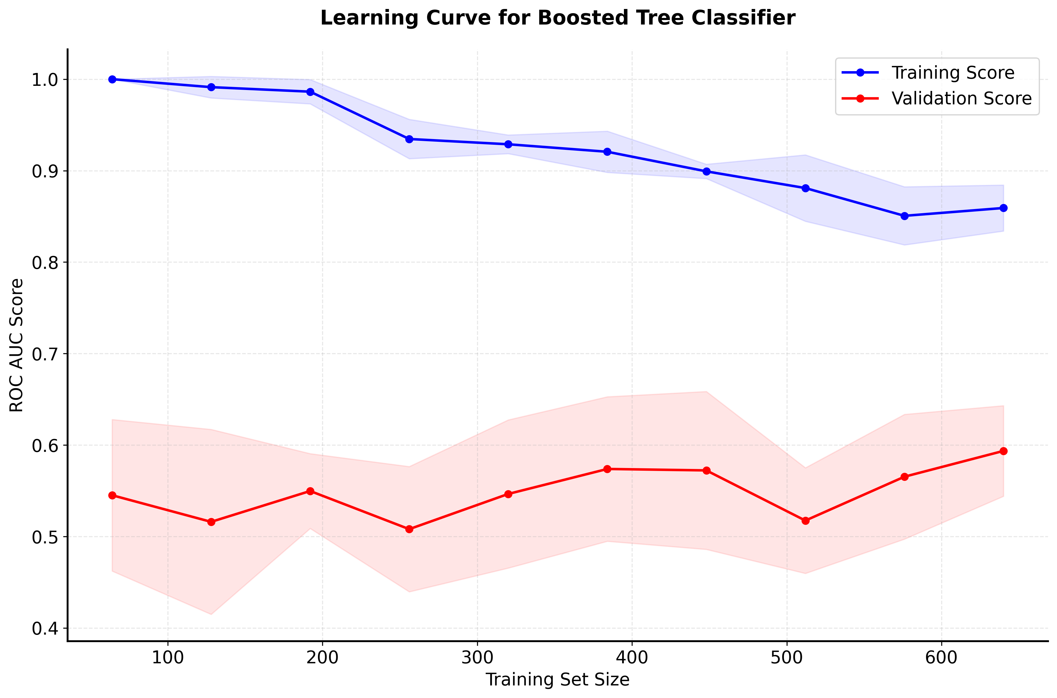
Early stopping provides a principled approach to determining the optimal number of trees. By monitoring validation set performance during training, you can halt the process when additional trees no longer improve generalization. This prevents overfitting while avoiding the need to manually specify the number of trees. Combine early stopping with subsampling (training each tree on 50-80% of the data) to introduce stochasticity that further reduces overfitting risk.

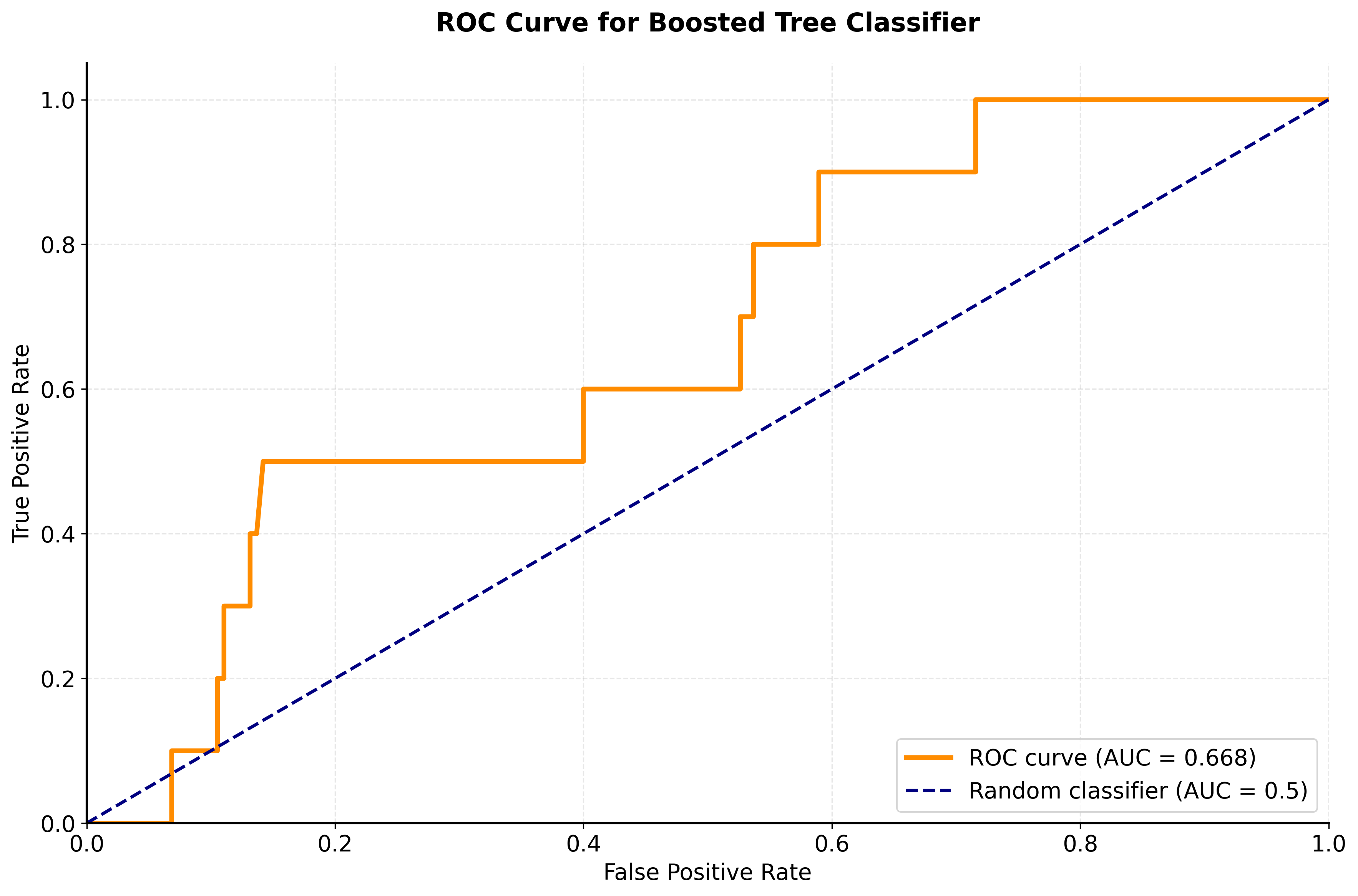
Evaluation should employ multiple metrics appropriate to the problem type. For classification, combine accuracy with precision, recall, and ROC AUC to understand performance across different decision thresholds. For regression, examine both R² and RMSE to assess explained variance and prediction error magnitude. Cross-validation provides robust performance estimates and helps detect overfitting, particularly when combined with stratified sampling for imbalanced classification problems.

Common Pitfalls

Overfitting represents the most common failure mode for boosted trees, manifesting as excellent training performance but poor generalization. This typically occurs when using too many trees, high learning rates, or insufficient regularization. The sequential nature of boosting means that later trees can memorize training noise rather than learning generalizable patterns. Combat this by implementing early stopping based on validation set performance, using lower learning rates with more trees, and applying tree-level regularization through depth limits and minimum sample requirements.

Computational efficiency becomes problematic for large datasets or when extensive hyperparameter tuning is required. Unlike Random Forest, which trains trees in parallel, boosted trees must train sequentially, making the process inherently slower. While individual tree training can leverage multiple cores through n_jobs, the overall boosting process remains serial. For large-scale applications, consider using modern implementations like XGBoost or LightGBM that employ algorithmic optimizations, or reduce dataset size through stratified sampling while ensuring representative coverage of the feature space.

The algorithm's sensitivity to data quality can undermine performance when training data contains outliers or labeling errors. Each tree attempts to correct previous errors, so systematic noise or outliers receive increasing attention as boosting progresses. This can cause the model to fit noise rather than signal. Address this through careful data cleaning, using robust loss functions that downweight extreme residuals, and monitoring feature importance to identify features that may be capturing noise rather than meaningful patterns.

Computational Considerations

Training complexity scales linearly with the number of trees and the size of the dataset, but the sequential nature of boosting prevents full parallelization. Each tree must wait for all previous trees to complete before training can begin. For datasets exceeding 100,000 samples, training time can become substantial, particularly when performing grid search over hyperparameters. Modern implementations like XGBoost and LightGBM address this through histogram-based algorithms and other optimizations that significantly reduce training time without sacrificing accuracy.

Memory requirements depend primarily on the number of trees and their depth. A typical model with 100 trees of depth 5 requires modest memory, but ensembles with thousands of trees or very deep trees can consume substantial resources. During training, the algorithm must store the entire dataset in memory along with residuals and predictions for each boosting iteration. For memory-constrained environments, consider using fewer trees, limiting tree depth, or employing out-of-core learning approaches that process data in batches.

Performance and Deployment Considerations

Inference speed requires evaluating all trees in the ensemble sequentially, with each tree traversing from root to leaf based on feature values. For real-time applications requiring sub-millisecond predictions, this can become a bottleneck. Model compression techniques like tree pruning or knowledge distillation can reduce the ensemble size while maintaining most of the predictive performance. Alternatively, caching predictions for common input patterns or using approximate nearest neighbor lookups can accelerate inference in production systems.

Model maintenance presents challenges because boosted trees cannot be updated incrementally—new data requires complete retraining. This differs from online learning algorithms that can update weights continuously. For applications requiring frequent updates, establish a retraining schedule that balances model freshness with computational cost. Monitor prediction performance on recent data to detect concept drift, which may indicate the need for retraining even before the scheduled update. Feature importance tracking across retraining cycles can reveal evolving patterns in the data and inform feature engineering efforts.

Summary

Boosted trees are a powerful and sophisticated ensemble learning algorithm that achieves exceptional predictive performance by sequentially building an ensemble of decision trees, with each new tree focusing on correcting the errors made by the previous trees. This iterative, error-correcting approach allows boosted trees to capture complex, non-linear relationships and feature interactions that simpler algorithms might miss.

The key strength of boosted trees lies in their ability to achieve state-of-the-art predictive accuracy across a wide variety of problems. The algorithm can handle both numerical and categorical features effectively, provides built-in feature importance measures, and offers flexibility in the choice of loss functions, making it adaptable to different types of problems.

However, boosted trees are prone to overfitting and require careful hyperparameter tuning to achieve optimal performance. The sequential nature of the algorithm makes training computationally expensive, and the models can be quite large and memory-intensive. Additionally, while boosted trees provide feature importance measures, the individual trees in the ensemble are not easily interpretable, and the sequential nature of the algorithm makes it difficult to understand the exact decision-making process.

Despite these limitations, boosted trees remain one of the most powerful and effective machine learning algorithms, often achieving the best performance on tabular data problems. Their combination of exceptional accuracy, flexibility, and robustness makes them particularly valuable in applications where predictive performance is the primary concern, such as in machine learning competitions, financial modeling, and other domains where accuracy is crucial. However, they require careful tuning and validation to prevent overfitting and ensure good generalization performance.