InteractiveLIME Explainability: Complete Guide to Local Interpretable Model-Agnostic Explanations

LIME (Local Interpretable Model-Agnostic Explanations)

Concept

LIME (Local Interpretable Model-Agnostic Explanations) is a technique for explaining the predictions of any machine learning model by creating simple, interpretable approximations around individual predictions. The core idea is that while complex models like deep neural networks or ensemble methods may be difficult to understand globally, we can often explain their behavior locally around a specific prediction by fitting a simple, interpretable model to that local region.

The method works by taking a specific instance we want to explain, generating variations of that instance by perturbing its features, and then fitting a simple linear model (like linear regression) to predict how the complex model behaves on these variations. This local linear model serves as an explanation for why the complex model made its prediction for that specific instance.

LIME is model-agnostic, meaning it can explain any machine learning model regardless of its internal structure. Whether we're working with a random forest, a neural network, or a support vector machine, LIME treats the model as a black box and only needs the model's input-output behavior to generate explanations.

The technique is valuable in high-stakes applications where understanding individual decisions matters. In healthcare, doctors need to know why a model recommended a specific treatment. In finance, regulators require explanations for loan denials. In autonomous vehicles, engineers need to understand why the system made a critical driving decision. LIME bridges the gap between the predictive power of complex models and the human need for transparent, interpretable reasoning.

Advantages

LIME offers several key advantages that make it a practical choice for model interpretability. First, its model-agnostic nature means we can apply it to any machine learning model without needing to understand or modify the model's internal structure. This universality makes LIME valuable in production environments where we might need to explain predictions from different types of models.

Second, LIME provides intuitive, human-readable explanations by using simple linear models locally. The feature weights in these local models directly correspond to how much each feature contributed to the prediction, making the explanations easy to understand and communicate to stakeholders. This interpretability is important for building trust in AI systems and ensuring regulatory compliance.

Third, LIME is computationally efficient for generating explanations of individual predictions. Unlike global explanation methods that might require retraining models or extensive computational resources, LIME can generate explanations quickly by sampling around the instance of interest and fitting a simple local model.

Disadvantages

LIME has several limitations that we should understand before using it:

The most significant disadvantage is that LIME provides only local explanations, meaning the explanations are valid only in the immediate neighborhood of the specific instance being explained. These local explanations do not generalize to other parts of the feature space, and the same model might behave very differently in other regions.

Another major limitation is LIME's sensitivity to the sampling strategy and parameters used to generate the local perturbations. The choice of how to perturb features, the number of samples generated, and the distance metric used can significantly affect the resulting explanations. This sensitivity means that different parameter choices can lead to different explanations for the same instance, potentially undermining the reliability of the method.

Additionally, LIME assumes that the local linear approximation is meaningful, which may not hold in all cases. If the complex model's decision boundary is highly non-linear in the local region, a linear approximation might miss important aspects of the model's behavior. This limitation is problematic for models with complex interactions between features or highly non-linear decision boundaries.

Formula

The mathematical foundation of LIME begins with a fundamental question: How do we fairly attribute a model's prediction to its input features when the model itself is a complex, opaque function? We need to explain not just which features matter, but precisely how much each feature contributes to a specific prediction in a way that is both accurate and interpretable.

Starting with the Core Problem

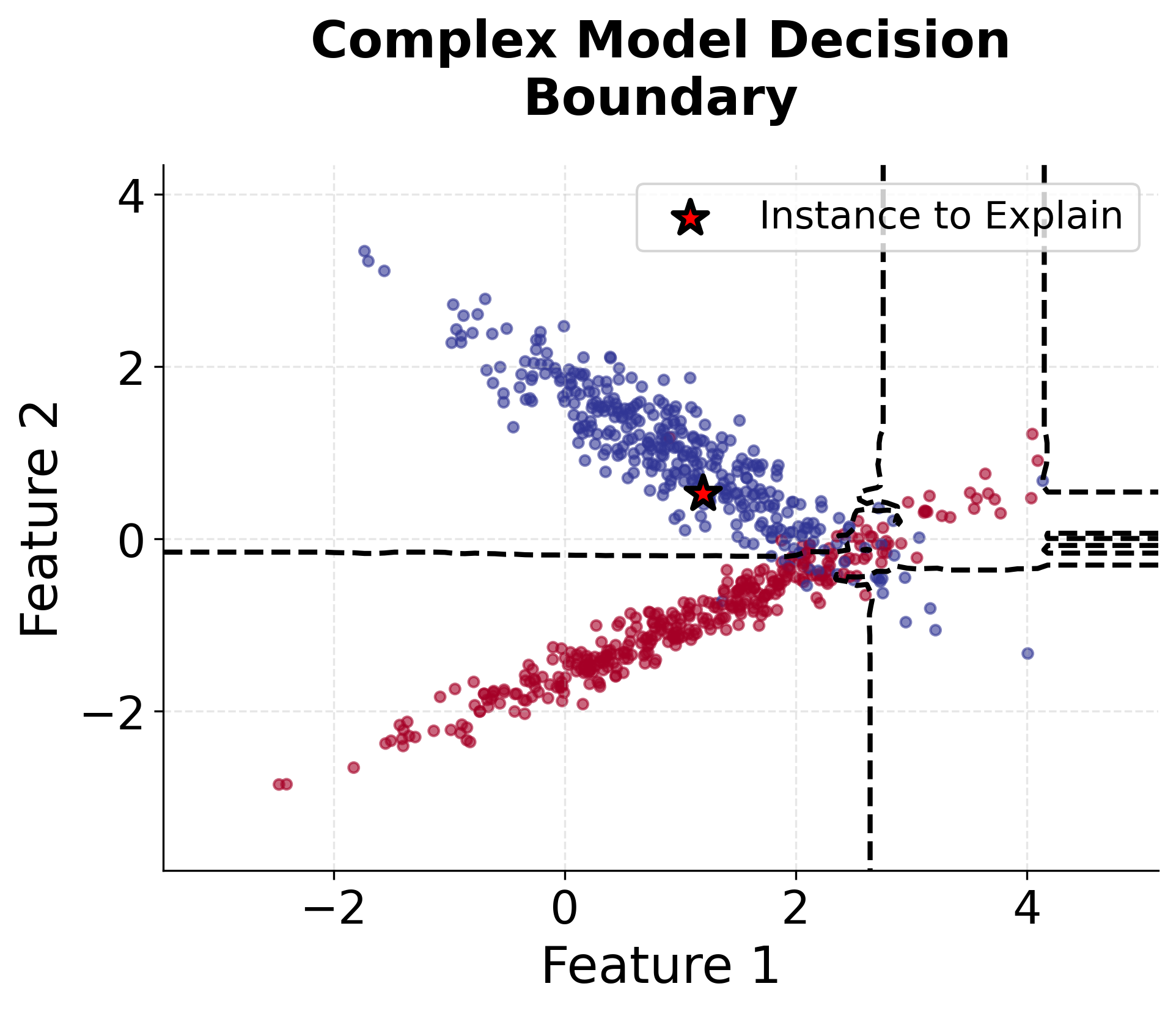
Explaining a complex model globally is often impossible. The intricate interactions between features, non-linear transformations, and complex decision boundaries resist simple explanations. LIME takes a different approach. Instead of trying to explain the entire model, we focus on understanding its behavior in a small neighborhood around a specific prediction.

Think of it this way. If you're standing on a mountainous terrain, the global landscape is complex and hard to describe. But if you look at the ground right around your feet, it appears nearly flat. LIME applies this same logic to machine learning models. Locally, even complex models often behave approximately linearly.

Building a Simple Explanation Model

We need a simple model $g$ that approximates our complex model $f$ in the local neighborhood. What makes a model both simple and interpretable? LIME chooses a linear model because linear models provide clear, additive feature contributions. We can write this as:

$g(z') = w_g \cdot z'$

where:

• $g$: Local explanation model (linear)
• $f$: Complex model we want to explain
• $z'$: Instance in simplified interpretable representation (typically binary vector)
• $w_g$: Weight vector containing attribution scores for each feature

Each weight $w_g[i]$ directly answers the question: "How much does feature $i$ contribute to this prediction?"

The linear form is key. It lets us understand the total prediction as a sum of individual feature contributions. If we say the prediction is 0.7, we can say "Feature 1 contributed +0.2, Feature 2 contributed +0.3, Feature 3 contributed +0.2." This additive structure makes the explanation naturally interpretable.

Defining "Local" with a Proximity Measure

Having a linear model isn't enough. We need to ensure it accurately represents the complex model's behavior where it matters most: near our instance of interest. Not all nearby instances should matter equally. An instance very similar to our original should influence the explanation much more than one that's only vaguely similar.

We capture this with a proximity measure $\pi_x(z)$ that quantifies how "local" each perturbed instance $z$ is to our original instance $x$. We typically use an exponential kernel:

$\pi_x(z) = \exp(-D(x, z)^2 / \sigma^2)$

where:

• $\pi_x(z)$: Proximity weight for instance $z$ relative to original instance $x$
• $D(x, z)$: Distance between original instance $x$ and perturbed instance $z$
• $\sigma$: Bandwidth parameter controlling the size of the local neighborhood

This formula captures our intuition well. When a perturbed instance $z$ is very close to $x$, the distance $D(x, z)$ is small. The exponential function returns a weight close to 1, giving that instance full influence. As $z$ moves farther away, the weight decays exponentially. Only truly local instances shape our explanation.

The bandwidth parameter $\sigma$ controls the size of our local neighborhood. Choose $\sigma$ too small, and we might overfit to noise in the immediate vicinity. Choose it too large, and we include instances that aren't meaningfully local, violating our assumption that the model behaves linearly nearby.

Measuring Explanation Quality with a Weighted Loss

Now we can define what makes our simple explanation $g$ a good approximation of the complex model $f$. We want $g$ to match $f$'s predictions on nearby instances, with more emphasis on instances closer to our original. This gives us a weighted loss function:

$L(f, g, \pi_x) = \sum_{z, z'} \pi_x(z) (f(z) - g(z'))^2$

where:

• $L(f, g, \pi_x)$: Weighted loss function measuring approximation quality
• $z$: Perturbed instance in original feature space
• $z'$: Perturbed instance in interpretable representation
• $f(z)$: Complex model's prediction for instance $z$
• $g(z')$: Local explanation model's prediction for instance $z'$

The squared term $(f(z) - g(z'))^2$ measures how well our simple explanation matches the complex model's prediction for each perturbed instance. The proximity weight $\pi_x(z)$ scales this error. Matching accuracy matters more for nearby instances. By minimizing this weighted loss, we force $g$ to approximate $f$ accurately in the local neighborhood, with precision increasing as we approach the instance we're explaining.

Adding Sparsity for Interpretability

Accuracy alone doesn't guarantee a useful explanation. Imagine our local linear model closely matches $f$ on all nearby instances, but does so using all features with non-zero weights, including marginally relevant ones. This explanation would be technically accurate but practically useless. It fails to identify the truly important features.

We need sparse attributions that highlight only the features that genuinely matter. This motivates a complexity penalty $\Omega(g)$ that encourages simpler explanations:

$\Omega(g) = \lambda \|w_g\|_0$

where:

• $\Omega(g)$: Complexity penalty encouraging sparse explanations
• $\lambda$: Regularization parameter balancing accuracy and simplicity
• $\|w_g\|_0$: L0 norm counting the number of non-zero weights

The term $\|w_g\|_0$ counts the number of non-zero weights. The parameter $\lambda$ balances accuracy against simplicity. This penalty embodies Occam's razor: among equally accurate explanations, prefer the simpler one. By penalizing the number of features, we force the explanation to focus on the most important contributions, filtering out noise and marginal effects.

The Complete Optimization Problem

We can now state LIME's complete optimization problem:

$\xi(x) = \arg\min_{g \in G} L(f, g, \pi_x) + \Omega(g)$

where:

• $\xi(x)$: The explanation for instance $x$
• $G$: Class of interpretable models (linear models in LIME)
• $L(f, g, \pi_x)$: Weighted loss measuring local fidelity
• $\Omega(g)$: Complexity penalty for sparsity

This formula represents LIME's solution to the attribution problem. We're looking for an explanation $g$ that minimizes two things:

1. Weighted loss $L(f, g, \pi_x)$: Ensures the explanation accurately represents the model's behavior in the local neighborhood. The proximity weights make sure accuracy is prioritized near the instance we're explaining.

2. Complexity penalty $\Omega(g)$: Ensures the explanation remains interpretable by highlighting only the most important feature contributions.

These two objectives pull in different directions. The loss term wants explanations that closely match the complex model's behavior. The complexity penalty wants simpler explanations with fewer features. The proximity measure ensures both objectives are evaluated in the context that matters: the local neighborhood.

Together, these components create an optimization problem whose solution gives us clear, interpretable attribution of feature contributions. The result accurately reflects how the complex model behaves for this specific instance while remaining simple enough for humans to understand.

Mathematical Properties

The LIME optimization problem has several properties that affect how we use it in practice:

Non-convexity and practical solutions. The L0 penalty in $\Omega(g)$ makes the optimization problem non-convex, which means finding the global optimum is hard. In practice, most implementations use L1 regularization instead, replacing $\|w_g\|_0$ with $\|w_g\|_1$ (the sum of absolute values). This L1 penalty still encourages sparsity but creates a convex optimization problem we can solve efficiently. The tradeoff is acceptable: we lose theoretical guarantees about finding the sparsest solution, but we gain computational tractability and reliable convergence.

Sensitivity to bandwidth choice. The bandwidth parameter $\sigma$ in the proximity measure significantly affects explanation quality. Choose it carefully to balance local accuracy and generalization. If $\sigma$ is too small, we overfit to noise in the immediate vicinity. The explanation captures random fluctuations rather than meaningful patterns. If $\sigma$ is too large, we include instances that aren't meaningfully local, violating the assumption that the model behaves linearly in the neighborhood. A good practice is to experiment with different values and check that explanations remain stable.

The linearity assumption. LIME assumes the complex model's behavior is approximately linear in the local neighborhood. This assumption doesn't always hold. Models with highly non-linear decision boundaries or complex feature interactions in the local region can violate it. When this happens, the linear explanation misses important aspects of the model's behavior, leading to misleading attributions. We should validate this assumption by checking the weighted loss. If it's consistently high, the linear approximation isn't capturing the model's local behavior well, and the explanations may not be trustworthy.

Visualizing LIME

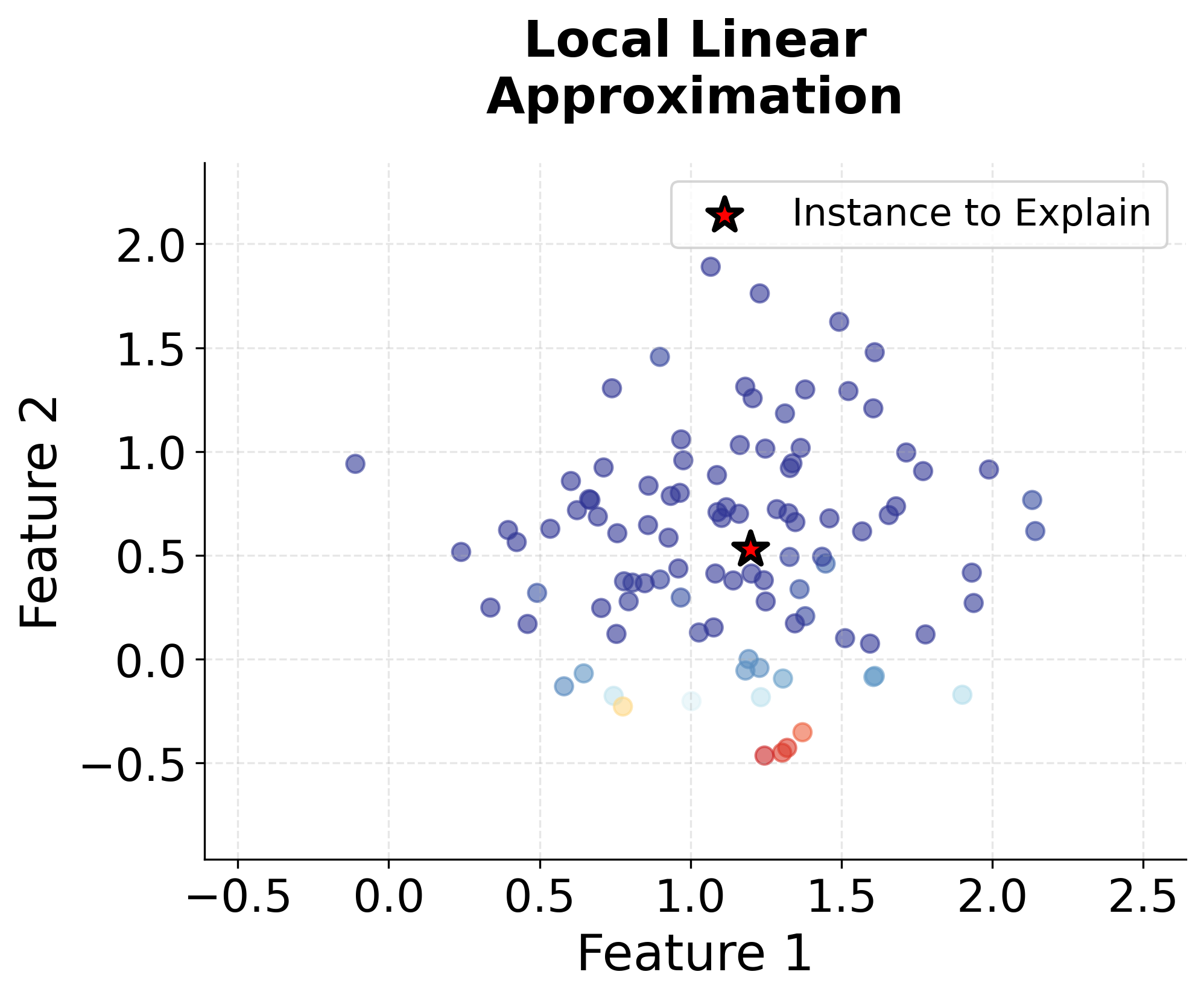
Let's create visualizations to understand how LIME works in practice. We'll start with a simple example using a 2D dataset to illustrate the core concepts.

Now let's visualize the feature importance weights that LIME would extract:

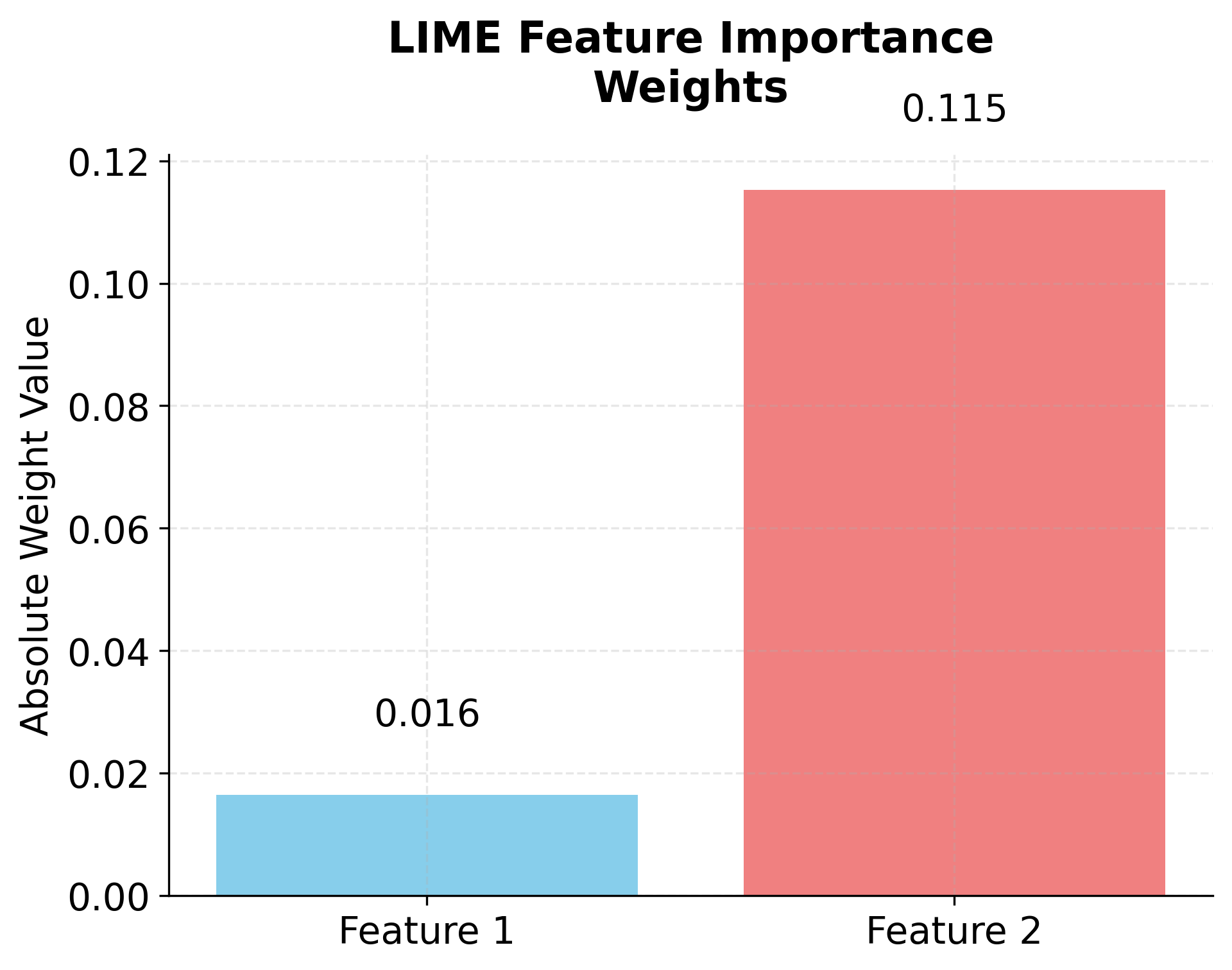
The local model coefficients show how much each feature contributes to the prediction in this neighborhood. The intercept represents the baseline prediction. We can compare the complex model's prediction with the local model's prediction to see how well our linear approximation captures the model's behavior. If they're close, our explanation is trustworthy for this instance.

Example

Let's walk through a concrete example of LIME step by step. We'll use a simple three-feature dataset to show exactly how LIME generates explanations.

We have a specific instance with three feature values. The complex model predicts a probability of belonging to the positive class, and we can compare this with the true label to see if the prediction is reasonable. Now let's implement LIME step by step to understand why the model made this prediction:

The local linear model gives us coefficients for each feature. These show their relative importance in explaining this prediction. Positive coefficients increase the probability, negative ones decrease it. The intercept is the baseline prediction when all features are zero. Notice how close the local model's prediction is to the complex model's prediction (shown earlier). This closeness tells us the linear approximation captures the model's behavior well in this local region.

Let's verify the quality of our approximation:

The weighted MSE measures how well our linear model approximates the complex model on the perturbed instances. A lower value means a better approximation. Here, the low MSE confirms our linear model captures the complex model's behavior well in this neighborhood.

The feature importance ranking shows which features drive the prediction. Features with larger absolute importance have stronger influence. The direction (positive or negative) tells us whether the feature increases or decreases the predicted probability.

Implementation using the Official LIME Package

The official LIME package (https://github.com/marcotcr/lime) provides a production-ready implementation for various data types. For tabular data, we use LimeTabularExplainer, which handles sampling, weighting, and local model fitting automatically.

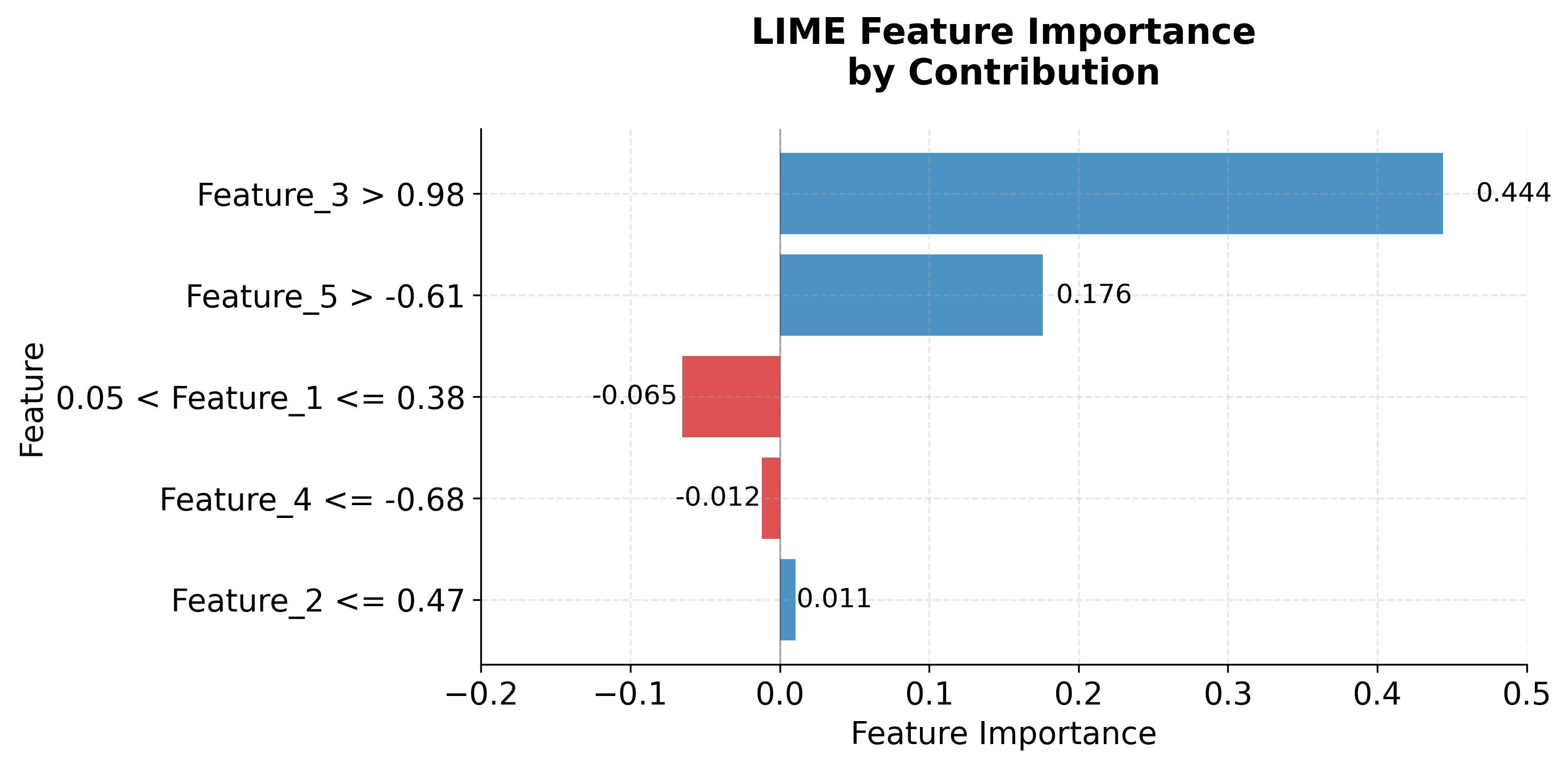
Now let's demonstrate the official LIME implementation with a practical example:

The feature importance list shows each feature and its contribution. Positive values mean the feature increases the probability of the predicted class. Negative values decrease it. The local model prediction should be close to the complex model prediction. When they match well, it means the linear approximation captures the model's behavior accurately.

Let's also visualize the explanation:

Key Parameters

Below are the main parameters that affect how LIME works and performs.

For LimeTabularExplainer:

• training_data (required): The training dataset. The explainer uses this to understand feature distributions and generate meaningful perturbations.
• feature_names (optional): List of feature names. Improves readability of explanations.
• mode (default: 'classification'): Either 'classification' or 'regression'. Determines how predictions are interpreted.
• kernel_width (default: 0.75): Width of the exponential kernel for weighting instances. Smaller values focus on very close instances. Larger values include more distant ones.
• discretize_continuous (default: True): Whether to discretize continuous features. Can improve explanations for some models.
• random_state (optional): Seed for reproducibility. Set to an integer for consistent results across runs.

For explain_instance():

• num_features (default: 10): Number of features to include in the explanation. More features give a more complete picture but may include less important ones.
• num_samples (default: 5000): Number of perturbed samples to generate. More samples improve quality but increase computation time. Values between 1000-5000 typically work well.

Key Methods

The following are the most commonly used methods for working with LIME.

• LimeTabularExplainer(training_data, ...): Initializes a LIME explainer for tabular data. Requires the training data and accepts optional parameters like feature names, mode, and kernel width.
• explain_instance(data_row, predict_fn, num_features=10, ...): Generates a LIME explanation for a single instance. Takes the instance to explain and the prediction function. Returns an Explanation object.
• explanation.as_list(): Returns the explanation as a list of (feature, importance) tuples, sorted by absolute importance. Useful for programmatic access.
• explanation.show_in_notebook(): Displays the explanation in interactive HTML format within Jupyter notebooks.
• explanation.as_pyplot_figure(): Creates a matplotlib visualization. Useful for static visualizations or non-notebook environments.

Practical Applications

LIME is particularly valuable when model interpretability matters for regulatory compliance, stakeholder communication, or debugging. In high-stakes applications where understanding individual predictions is critical, LIME provides a way to explain black-box model decisions without requiring access to the model's internal structure. This makes it especially useful in regulated industries where model transparency is required but proprietary models or ensemble methods make global interpretability impractical.

In healthcare, LIME helps clinicians understand why a model recommended a specific diagnosis or treatment. A doctor can examine which patient characteristics (age, lab results, medical history) contributed most to a prediction and validate whether the model's reasoning aligns with clinical knowledge. Similarly, in finance, LIME explains why a loan application was rejected or why a transaction was flagged as suspicious. These explanations support both regulatory compliance requirements and customer communication, helping financial institutions demonstrate that decisions aren't based on protected characteristics or unfair criteria.

LIME is also highly effective for model validation and debugging during development. By examining explanations across multiple instances, data scientists can identify when models make decisions based on spurious correlations or unexpected feature combinations. For example, if a medical diagnosis model consistently identifies the hospital ID as important, this reveals data leakage. This diagnostic capability helps catch issues before deployment, improving model reliability and trustworthiness in production systems.

Best Practices

To achieve reliable and interpretable explanations with LIME, always standardize your continuous features before generating explanations. LIME's distance calculations are sensitive to feature scales, so features with larger ranges will disproportionately influence the proximity measure. Use StandardScaler to normalize features to zero mean and unit variance. Without standardization, a feature measured in thousands (like annual income) will dominate one measured in decimals (like interest rate), even if both are equally important for the prediction.

Running LIME multiple times with different random seeds helps assess explanation stability. Because LIME uses stochastic sampling to generate perturbations, explanations can vary between runs. If the top features change dramatically across runs, the explanations may not be reliable indicators of true feature importance. Use at least 1000-5000 perturbation samples (controlled by num_samples) to reduce variability. Monitor the weighted MSE to verify that the local linear model adequately approximates the complex model's behavior in the neighborhood. A consistently high MSE suggests the linear approximation assumption is violated, making the explanations potentially misleading.

Always validate LIME's identified important features against domain knowledge. Features that appear important should make intuitive sense given the problem context. If LIME consistently highlights unexpected features (like record IDs or timestamps), this often reveals issues with the underlying model such as data leakage or spurious correlations. Use these insights to improve your model before deploying it. For critical applications, combine LIME with other explanation methods like SHAP to cross-validate findings and ensure robust interpretation of model behavior.

Data Requirements and Preprocessing

LIME requires numerical features for its distance-based proximity calculations, so categorical features must be encoded before generating explanations. One-hot encoding is the standard approach for nominal categories, though it increases feature dimensionality. For datasets with many categorical features, this can create sparse, high-dimensional representations that make distance calculations less meaningful. For ordinal categorical variables where the ordering is meaningful (like education level or product rating), label encoding preserves the ordinality while maintaining a single dimension per feature.

Mixed data types require careful consideration of how distances are calculated. The default Euclidean distance treats all features as continuous, which may not be appropriate for binary or categorical features even after encoding. Some implementations allow custom distance metrics that handle mixed types more appropriately, weighting categorical and continuous features differently. Features with highly skewed distributions can also affect explanation quality because extreme values create large distances. Log transformation or other normalizing transformations help reduce the impact of outliers and make the distance calculations more robust. Missing values must be handled before applying LIME, either through imputation or by removing instances with missing data, as LIME cannot directly handle missing values in its distance calculations.

Common Pitfalls

One of the most common mistakes is using too few perturbation samples, which leads to noisy and unstable explanations. While reducing the number of samples decreases computation time, it also reduces the quality of the local approximation. The default value of 5000 samples in the LIME package is reasonable for most applications, but some practitioners reduce this to save time without checking explanation stability. Start with at least 1000 samples and verify that explanations remain consistent across multiple runs before reducing this value further. If you see large changes in feature importance rankings between runs, increase the number of samples.

Another frequent issue is choosing an inappropriate bandwidth parameter (controlled by kernel_width in the LIME implementation). The bandwidth determines the size of the local neighborhood, and getting it wrong undermines the entire approach. If the bandwidth is too small, LIME focuses on a very narrow region and may overfit to noise or random fluctuations in the model's predictions. If it's too large, the neighborhood includes instances where the model's behavior is no longer approximately linear, violating LIME's core assumption. The default value of 0.75 works reasonably well for many cases, but you should validate this by examining the weighted MSE. Experiment with different values (try 0.5, 0.75, 1.0) and choose the one that provides stable explanations with acceptable approximation error.

Perhaps the most problematic mistake is treating LIME explanations as globally valid insights into model behavior. Each LIME explanation is valid only in the local neighborhood around the specific instance being explained. The model might use completely different features or decision logic in other parts of the feature space. For example, an explanation showing that "age is the most important feature" for one loan application tells you nothing about whether age matters for other applications. To understand global patterns, examine explanations across many representative instances or use global explanation methods like SHAP or permutation feature importance instead.

Computational Considerations

LIME's computational complexity scales linearly with the number of perturbation samples and the number of features, making it relatively efficient for individual explanations. With the default 5000 perturbation samples and a typical model, generating a single explanation usually takes 1-5 seconds on modern hardware. The main computational bottlenecks are generating perturbations, obtaining predictions from the complex model for each perturbed instance, and fitting the local linear model. For datasets where you need to explain thousands of instances, the total computation time becomes substantial. Explaining 1000 instances with 5000 samples each requires 5 million model predictions, which can take minutes to hours depending on your model's prediction speed.

For large-scale applications, several strategies can reduce computational costs. First, reduce the number of perturbation samples to 1000-2000 if your model's predictions are relatively stable and smooth in local regions. Test this by comparing explanations with different sample sizes to ensure quality doesn't degrade significantly. Second, implement caching for frequently explained instances, since explanations for identical instances with identical parameters are deterministic (given the same random seed). This is particularly useful in production systems where certain types of queries are common. Third, leverage parallelization when explaining multiple instances, as each explanation is independent and can be computed concurrently. The LIME package doesn't parallelize automatically, but you can use Python's multiprocessing or joblib to distribute explanations across CPU cores.

For very large-scale applications (tens of thousands of explanations), consider using approximate methods or alternative explanation approaches. Some practitioners use a two-stage approach: apply LIME to a representative sample of instances to understand general patterns, then use faster methods like permutation importance for routine monitoring. Alternatively, for models where training time is acceptable, consider using inherently interpretable models like linear models or decision trees for critical applications where explanations are frequently needed.

Performance and Deployment Considerations

LIME explanations are instance-specific and must be generated on-demand, which directly impacts application responsiveness in production environments. For interactive applications where users expect immediate explanations (such as loan officers reviewing credit decisions or doctors examining diagnosis recommendations), aim for explanation generation times under 2-3 seconds. If generation takes longer, users may abandon the explanation feature or lose trust in the system. Reduce the number of perturbation samples to 1000-2000 for faster generation, though you should validate that this maintains acceptable explanation quality. Implement explanation caching for common query patterns, particularly useful when certain types of instances are frequently queried.

When deploying LIME in production, monitor explanation quality and stability over time. Changes in the underlying model (such as retraining with new data) or shifts in the data distribution can affect explanation quality and consistency. Track metrics like the weighted MSE to detect when the linear approximation quality degrades. Monitor feature importance stability by logging the top features identified for similar instances over time. Sudden changes in these patterns may indicate model drift or data quality issues that require investigation. Set up alerts when the average weighted MSE exceeds historical thresholds or when explanation stability drops below acceptable levels.

Consider the interpretability-accuracy tradeoff when choosing models for production use. Highly complex models with many interactions and non-linearities may produce accurate predictions but generate less reliable LIME explanations because the local linear approximation fails to capture the model's behavior adequately. In regulated domains where explanation quality is critical, you may need to accept slightly lower predictive accuracy in exchange for more reliable explanations by using simpler models or ensemble methods that are easier to approximate locally. Also ensure that explanations don't inadvertently reveal sensitive information about the training data or model internals that could be exploited or create privacy concerns, particularly when explanations are shared with external stakeholders or customers.

Summary

LIME provides a framework for generating local, interpretable explanations of complex machine learning models. It approximates model behavior with simple linear models in local neighborhoods. The method's model-agnostic nature makes it applicable to a wide range of algorithms. Its linear explanations are accessible to non-technical stakeholders.

The mathematical foundation centers on optimizing a weighted loss function that balances local approximation accuracy with explanation simplicity. Exponential kernels weight instances by their proximity to the instance being explained. This ensures the local linear model captures the complex model's behavior in the relevant neighborhood.

LIME offers advantages in interpretability and model-agnostic applicability. However, be aware of its limitations:

• Sensitivity to sampling parameters
• Assumption of local linearity
• Computational overhead for generating explanations

Successful deployment requires careful consideration of data preprocessing, model selection, and validation strategies. Ensure the generated explanations are both accurate and meaningful for your use case.