InteractiveMultinomial Logistic Regression: Complete Guide with Mathematical Foundations & Python Implementation

Multinomial Logistic Regression

Multinomial logistic regression is a powerful extension of binary logistic regression that allows us to model relationships between multiple categorical outcomes and predictor variables. While binary logistic regression handles situations with exactly two possible outcomes (like "yes" or "no"), multinomial logistic regression extends this capability to handle three or more mutually exclusive categories. This makes it invaluable for classification problems where we need to predict which of several possible classes an observation belongs to.

The key insight behind multinomial logistic regression is that we can model the probability of each category relative to a reference category. Unlike binary logistic regression, which uses a single logistic function, multinomial logistic regression uses multiple logistic functions simultaneously. Each function represents the log-odds of one category compared to the reference category, creating a system of equations that must be solved together.

This approach is particularly useful in fields like marketing (predicting customer segments), medicine (diagnosing disease types), and natural language processing (classifying text into different topics). The model assumes that the categories are mutually exclusive and collectively exhaustive, meaning each observation must belong to exactly one category, and all possible categories are included in the model.

Advantages

Multinomial logistic regression offers several compelling advantages over alternative classification methods. First, it provides interpretable probability estimates for each class, not just the predicted class. This probabilistic output is crucial in many applications where we need to understand the confidence of our predictions or make decisions based on uncertainty. For example, in medical diagnosis, knowing that a patient has a 60% chance of having condition A, 30% chance of condition B, and 10% chance of condition C is much more informative than simply predicting condition A.

Second, the model naturally handles the constraint that all class probabilities must sum to one, ensuring that our predictions are mathematically consistent. This built-in constraint prevents the common problem of having probabilities that don't add up correctly, which can occur with other multi-class approaches that treat each class independently. Additionally, multinomial logistic regression can handle both categorical and continuous predictor variables seamlessly, making it flexible for diverse datasets.

Finally, the model provides direct interpretability through odds ratios, allowing us to understand how changes in predictor variables affect the relative probability of different outcomes. This interpretability is particularly valuable in fields where understanding the relationship between variables is as important as making accurate predictions.

Disadvantages

Despite its strengths, multinomial logistic regression has several limitations that practitioners should consider. The most significant disadvantage is the assumption of independence of irrelevant alternatives (IIA), which states that the relative probabilities of any two alternatives should not change when a third alternative is added or removed. This assumption can be violated in many real-world scenarios, particularly when alternatives are similar or when there are unobserved factors that affect multiple alternatives similarly.

Another limitation is the model's sensitivity to the choice of reference category. While the choice of reference category doesn't affect the overall model fit, it can significantly impact the interpretation of coefficients and odds ratios. This can make model interpretation more complex, especially when communicating results to stakeholders who may not be familiar with the reference category concept.

Additionally, multinomial logistic regression can become computationally intensive as the number of categories increases, since we need to estimate parameters for each category relative to the reference. The model also assumes linear relationships between the log-odds and predictor variables, which may not hold in all situations. When these assumptions are violated, the model's performance can degrade significantly, and alternative approaches like decision trees or neural networks might be more appropriate.

Formula

The mathematical foundation of multinomial logistic regression builds upon the principles of binary logistic regression, but extends them to handle multiple categories. Let's walk through the derivation step by step, starting with the most intuitive form and progressing to the matrix notation.

Basic Probability Model

We begin with the fundamental assumption that we have $K$ categories (where $K \geq 3$) and want to model the probability that observation $i$ belongs to category $k$. Let's denote this probability as $P(y_i = k | \mathbf{x}_i)$, where $\mathbf{x}_i$ represents the vector of predictor variables for observation $i$.

The key insight is that we can model the log-odds of each category relative to a reference category. Without loss of generality, let's choose category $K$ as our reference category. The log-odds of category $k$ relative to category $K$ is:

$\log\left(\frac{P(y_i = k | \mathbf{x}_i)}{P(y_i = K | \mathbf{x}_i)}\right) = \beta_{k0} + \beta_{k1}x_{i1} + \beta_{k2}x_{i2} + \cdots + \beta_{kp}x_{ip}$

where:

• $P(y_i = k | \mathbf{x}_i)$ is the probability that observation $i$ belongs to category $k$ given its predictor values (the conditional probability we're modeling for the non-reference category)
• $P(y_i = K | \mathbf{x}_i)$ is the probability that observation $i$ belongs to the reference category $K$ (the baseline category against which all others are compared)
• $\beta_{k0}$ is the intercept for category $k$ (the baseline log-odds when all predictors are zero)
• $\beta_{kj}$ is the coefficient for predictor $j$ in category $k$ (quantifies the effect of predictor $j$ on the log-odds of category $k$ relative to the reference category)
• $x_{ij}$ is the value of predictor $j$ for observation $i$ (the observed feature value)
• $p$ is the total number of predictor variables (the dimensionality of the feature space)
• $K$ is the reference category (chosen arbitrarily, typically the last category, with all its coefficients set to zero for identifiability)

From Log-Odds to Probabilities

To convert these log-odds back to probabilities, we need to solve for $P(y_i = k | \mathbf{x}_i)$. Let's define the linear predictor for category $k$ as:

$\eta_{ik} = \beta_{k0} + \beta_{k1}x_{i1} + \beta_{k2}x_{i2} + \cdots + \beta_{kp}x_{ip}$

where:

• $\eta_{ik}$ is the linear predictor for observation $i$ and category $k$ (a real-valued quantity that can take any value from $-\infty$ to $+\infty$, representing the log-odds before normalization)

Then we can write:

$\log\left(\frac{P(y_i = k | \mathbf{x}_i)}{P(y_i = K | \mathbf{x}_i)}\right) = \eta_{ik}$

Taking the exponential of both sides:

$\frac{P(y_i = k | \mathbf{x}_i)}{P(y_i = K | \mathbf{x}_i)} = e^{\eta_{ik}}$

This gives us:

$P(y_i = k | \mathbf{x}_i) = P(y_i = K | \mathbf{x}_i) \cdot e^{\eta_{ik}}$

Normalization Constraint

Since all probabilities must sum to one, we have:

$\sum_{k=1}^{K} P(y_i = k | \mathbf{x}_i) = 1$

Substituting our expression for $P(y_i = k | \mathbf{x}_i)$:

$\sum_{k=1}^{K} P(y_i = K | \mathbf{x}_i) \cdot e^{\eta_{ik}} = 1$

Since $P(y_i = K | \mathbf{x}_i)$ is common to all terms, we can factor it out:

$P(y_i = K | \mathbf{x}_i) \sum_{k=1}^{K} e^{\eta_{ik}} = 1$

This gives us the probability of the reference category:

$P(y_i = K | \mathbf{x}_i) = \frac{1}{\sum_{k=1}^{K} e^{\eta_{ik}}}$

Final Probability Formula

Now we can express the probability of any category $k$ as:

$P(y_i = k | \mathbf{x}_i) = \frac{e^{\eta_{ik}}}{\sum_{j=1}^{K} e^{\eta_{ij}}}$

This is the softmax function, which ensures that all probabilities sum to one and are non-negative. Notice that when $K = 2$, this reduces to the standard logistic regression formula.

Matrix Notation

For computational efficiency and clarity, we can express the multinomial logistic regression model in matrix notation.

Let $\mathbf{X}$ be the $n \times (p+1)$ design matrix, where $n$ is the number of observations and $p$ is the number of predictors (the extra column accounts for the intercept). For each non-reference category $k$ (where $k = 1, \ldots, K-1$), let $\boldsymbol{\beta}_k$ be a $(p+1) \times 1$ vector of coefficients. We stack these coefficient vectors horizontally to form a $(p+1) \times (K-1)$ coefficient matrix:

where:

• $\mathbf{X}$ is the $n \times (p+1)$ design matrix (includes a column of 1s for the intercept term, allowing matrix multiplication to compute all linear predictors)
• $n$ is the number of observations in the dataset (the sample size)
• $p$ is the number of predictor variables (the number of features, excluding the intercept)
• $\boldsymbol{\beta}_k$ is the $(p+1) \times 1$ coefficient vector for category $k$ (includes the intercept $\beta_{k0}$ as the first element, followed by $p$ slope coefficients)
• $\boldsymbol{\beta}$ is the $(p+1) \times (K-1)$ coefficient matrix for all non-reference categories (each column is a coefficient vector $\boldsymbol{\beta}_k$ for one non-reference category)
• $K$ is the total number of categories (including the reference category)

The linear predictors for all observations and all non-reference categories can be computed as:

where:

• $\boldsymbol{\eta}$ is the $n \times (K-1)$ matrix of linear predictors (each row corresponds to one observation, each column corresponds to one non-reference category, and element $\eta_{ik}$ is the linear predictor for observation $i$ and category $k$)

To obtain the predicted probabilities for all $K$ categories, we apply the softmax function row-wise. For each observation $i$ and category $k$:

where for the reference category $K$, we set $\eta_{iK} = 0$ (since its coefficients are all zero by convention).

In matrix notation, the full $n \times K$ probability matrix $\mathbf{P}$, with elements $P_{ik} = P(y_i = k \mid \mathbf{x}_i)$, is given by:

where:

• $\mathbf{P}$ is the $n \times K$ probability matrix (each row contains the predicted probabilities for one observation across all $K$ categories)
• $P_{ik}$ is the probability that observation $i$ belongs to category $k$ (an element of the probability matrix)
• $[\boldsymbol{\eta}, \mathbf{0}]$ is the $n \times K$ matrix formed by horizontally concatenating $\boldsymbol{\eta}$ (the $n \times (K-1)$ matrix of linear predictors for non-reference categories) with $\mathbf{0}$ (a column of zeros for the reference category)
• $\mathbf{0}$ is the $n \times 1$ column vector of zeros for the reference category (representing $\eta_{iK} = 0$ for all observations)
• $\text{softmax}(\cdot)$ is the softmax function applied row-wise (transforms linear predictors into probabilities that are non-negative and sum to 1 for each observation)

This formulation ensures that all predicted probabilities are non-negative and sum to one for each observation.

This matrix-based approach is highly efficient for computation, especially when working with large datasets or when fitting the model using optimization algorithms that require gradients with respect to all parameters.

Calculating the Coefficients

The coefficients in multinomial logistic regression are estimated using maximum likelihood estimation (MLE). This process involves finding the parameter values that maximize the likelihood of observing our data given the model.

Likelihood Function

For a dataset with $n$ observations and $K$ classes, the likelihood function is:

$L(\boldsymbol{\beta}) = \prod_{i=1}^{n} \prod_{k=1}^{K} P(y_i = k | \mathbf{x}_i)^{I(y_i = k)}$

where:

• $L(\boldsymbol{\beta})$ is the likelihood function (the probability of observing the entire dataset given the model parameters $\boldsymbol{\beta}$)
• $\boldsymbol{\beta}$ represents all coefficient parameters in the model (the collection of all $\beta_{kj}$ values for all non-reference categories and all predictors)
• $n$ is the number of observations (the sample size)
• $K$ is the number of categories (the total number of possible outcome classes)
• $P(y_i = k | \mathbf{x}_i)$ is the predicted probability that observation $i$ belongs to category $k$ (computed using the softmax function)
• $I(y_i = k)$ is the indicator function that equals 1 if observation $i$ truly belongs to class $k$, and 0 otherwise (selects the probability of the observed class)

Log-Likelihood Function

Working with the log-likelihood is computationally more convenient:

$\ell(\boldsymbol{\beta}) = \sum_{i=1}^{n} \sum_{k=1}^{K} I(y_i = k) \log P(y_i = k | \mathbf{x}_i)$

where:

• $\ell(\boldsymbol{\beta})$ is the log-likelihood function (the natural logarithm of the likelihood function, which transforms products into sums for computational convenience and numerical stability)

Substituting the softmax probability formula:

$\ell(\boldsymbol{\beta}) = \sum_{i=1}^{n} \sum_{k=1}^{K} I(y_i = k) \left[ \eta_{ik} - \log\left(\sum_{j=1}^{K} e^{\eta_{ij}}\right) \right]$

Gradient and Hessian

To find the maximum likelihood estimates, we need the gradient (first derivatives) and Hessian (second derivatives) of the log-likelihood function.

Let's break down how to compute the gradient and Hessian of the multinomial logistic regression log-likelihood step by step.

Step 1: Recall the log-likelihood

The log-likelihood for multinomial logistic regression is:

where $I(y_i = k)$ is 1 if observation $i$ belongs to class $k$, and 0 otherwise.

Step 2: Substitute the softmax probability

Recall that

where:

• $\eta_{ik} = \mathbf{x}_i^\top \boldsymbol{\beta}_k$ is the linear predictor for observation $i$ and category $k$ (computed as the dot product of the feature vector and coefficient vector)
• $\mathbf{x}_i^\top$ is the transpose of the feature vector for observation $i$ (a $1 \times (p+1)$ row vector including a 1 for the intercept)
• $\boldsymbol{\beta}_k$ is the coefficient vector for category $k$ (a $(p+1) \times 1$ column vector including the intercept and $p$ slope coefficients)

Step 3: Compute the gradient (first derivative) with respect to $\beta_{kj}$

We want to find the derivative of the log-likelihood with respect to a particular coefficient $\beta_{kj}$ (the coefficient for predictor $j$ in class $k$):

• The log-likelihood for a single observation $i$ is:

  $$\sum_{k=1}^K I(y_i = k) \log P(y_i = k | \mathbf{x}_i)$$

• The derivative with respect to $\beta_{kj}$ is:

  $$\frac{\partial}{\partial \beta_{kj}} \left[ I(y_i = k) \log P(y_i = k | \mathbf{x}_i) \right]$$

• Since $P(y_i = k | \mathbf{x}_i)$ depends on all $\beta_{kj}$, but only directly on $\beta_{kj}$ through $\eta_{ik}$, we use the chain rule.

• The derivative of $\log P(y_i = k | \mathbf{x}_i)$ with respect to $\beta_{kj}$ is:

  $$\frac{\partial}{\partial \beta_{kj}} \log P(y_i = k | \mathbf{x}_i) = x_{ij} \left[ I(y_i = k) - P(y_i = k | \mathbf{x}_i) \right]$$

  (This comes from differentiating the log-softmax.)

• Summing over all observations, we get:

  $$\frac{\partial \ell}{\partial \beta_{kj}} = \sum_{i=1}^{n} x_{ij} \left[ I(y_i = k) - P(y_i = k | \mathbf{x}_i) \right]$$

Step 4: Compute the Hessian (second derivative) with respect to $\beta_{kj}$ and $\beta_{lm}$

• The Hessian entry for parameters $\beta_{kj}$ and $\beta_{lm}$ is the second derivative: $$\frac{\partial^2 \ell}{\partial \beta_{kj} \partial \beta_{lm}}$$
• Differentiating the gradient again, we get: $$-\sum_{i=1}^{n} x_{ij} x_{im} P(y_i = k | \mathbf{x}_i) \left[ I(k = l) - P(y_i = l | \mathbf{x}_i) \right]$$ where $I(k = l)$ is 1 if $k = l$, and 0 otherwise.

Results:

• Gradient (First Derivatives):

  $$\frac{\partial \ell}{\partial \beta_{kj}} = \sum_{i=1}^{n} x_{ij} \left[ I(y_i = k) - P(y_i = k | \mathbf{x}_i) \right]$$

  where:

  • $\frac{\partial \ell}{\partial \beta_{kj}}$ is the partial derivative of the log-likelihood with respect to coefficient $\beta_{kj}$ (the gradient component for this parameter)
  • $\beta_{kj}$ is the coefficient for predictor $j$ in category $k$ (the parameter we're taking the derivative with respect to)
  • $x_{ij}$ is the value of predictor $j$ for observation $i$ (the feature value that multiplies this coefficient)
  • $I(y_i = k)$ is the indicator function (equals 1 if observation $i$ truly belongs to category $k$, and 0 otherwise)
  • $P(y_i = k | \mathbf{x}_i)$ is the predicted probability for observation $i$ in category $k$ (computed using the current parameter values)

• Hessian (Second Derivatives):

  $$\frac{\partial^2 \ell}{\partial \beta_{kj} \partial \beta_{lm}} = -\sum_{i=1}^{n} x_{ij} x_{im} P(y_i = k | \mathbf{x}_i) \left[ I(k = l) - P(y_i = l | \mathbf{x}_i) \right]$$

  where:

  • $\frac{\partial^2 \ell}{\partial \beta_{kj} \partial \beta_{lm}}$ is the second partial derivative of the log-likelihood (measures the curvature of the log-likelihood surface with respect to parameters $\beta_{kj}$ and $\beta_{lm}$)
  • $\beta_{lm}$ is the coefficient for predictor $m$ in category $l$ (the second parameter in the mixed partial derivative)
  • $x_{im}$ is the value of predictor $m$ for observation $i$ (the feature value that multiplies coefficient $\beta_{lm}$)
  • $I(k = l)$ is the indicator function (equals 1 if categories $k$ and $l$ are the same, and 0 otherwise)

Optimization Methods

The coefficients are found by maximizing the log-likelihood function using numerical optimization methods:

1. Newton-Raphson Method: Uses both gradient and Hessian information for faster convergence
2. Fisher Scoring: Uses the expected Fisher information matrix instead of the observed Hessian
3. Gradient Descent: Iteratively updates parameters in the direction of the gradient
4. Limited-memory BFGS (L-BFGS): A quasi-Newton method that approximates the Hessian

Iterative Reweighted Least Squares (IRLS)

Multinomial logistic regression can also be solved using IRLS, which reformulates the problem as a series of weighted least squares problems. This approach:

1. Starts with initial coefficient estimates
2. Computes fitted probabilities using the current coefficients
3. Creates working responses and weights
4. Solves a weighted least squares problem
5. Updates the coefficients
6. Repeats until convergence

Convergence Criteria

The optimization process continues until one of the following convergence criteria is met:

• Parameter convergence: $|\boldsymbol{\beta}^{(t+1)} - \boldsymbol{\beta}^{(t)}| < \epsilon$
• Log-likelihood convergence: $|\ell^{(t+1)} - \ell^{(t)}| < \epsilon$
• Gradient convergence: $|\nabla \ell^{(t)}| < \epsilon$

where:

• $\boldsymbol{\beta}^{(t)}$ is the vector of coefficient estimates at iteration $t$ (the current parameter values during optimization)
• $\boldsymbol{\beta}^{(t+1)}$ is the vector of coefficient estimates at iteration $t+1$ (the updated parameter values after one optimization step)
• $\ell^{(t)}$ is the log-likelihood value at iteration $t$ (the objective function value at the current parameters)
• $\ell^{(t+1)}$ is the log-likelihood value at iteration $t+1$ (the objective function value at the updated parameters)
• $\nabla \ell^{(t)}$ is the gradient vector at iteration $t$ (the vector of partial derivatives of the log-likelihood with respect to all parameters)
• $\epsilon$ is the tolerance threshold (a small positive number, typically $10^{-6}$ or $10^{-8}$, that determines when convergence is achieved)
• $|\cdot|$ denotes the absolute value (for scalars) or norm (for vectors), measuring the magnitude of change

Identifiability and Constraints

The multinomial logistic regression model is said to be overparameterized because, without any constraints, there are more parameters in the model than are actually needed to describe the relationship between the predictors and the outcome categories. Specifically, for $K$ outcome categories, the model estimates a separate set of coefficients for each category, but only $K-1$ of these sets are necessary to uniquely determine the predicted probabilities. This redundancy means that different sets of coefficients can produce the same predicted probabilities, making the model unidentifiable unless we impose a constraint.

To resolve this, the standard approach is to set the coefficients for one of the categories—called the reference category—to zero:

$\boldsymbol{\beta}_K = \mathbf{0}$

where:

• $\boldsymbol{\beta}_K$ is the coefficient vector for the reference category $K$ (a $(p+1) \times 1$ vector set to all zeros to ensure model identifiability)
• $\mathbf{0}$ is the zero vector (a $(p+1) \times 1$ vector with all elements equal to zero)

By doing this, we remove the redundancy and ensure that the model is identifiable, meaning the optimization problem has a unique solution and the estimated coefficients are interpretable relative to the reference category.

Mathematical Properties

The multinomial logistic regression model has several important mathematical properties. First, the softmax function ensures that all predicted probabilities are between 0 and 1 and sum to 1, which is necessary for a valid probability model. Second, the model is identifiable only up to the choice of reference category - we can add any constant to all coefficients without changing the predicted probabilities, which is why we typically set the coefficients for the reference category to zero.

The model also exhibits the property of proportional odds in the sense that the ratio of probabilities for any two categories depends only on the difference in their linear predictors. This means that if we change a predictor variable, the relative probabilities of all non-reference categories change proportionally, maintaining their relative relationships.

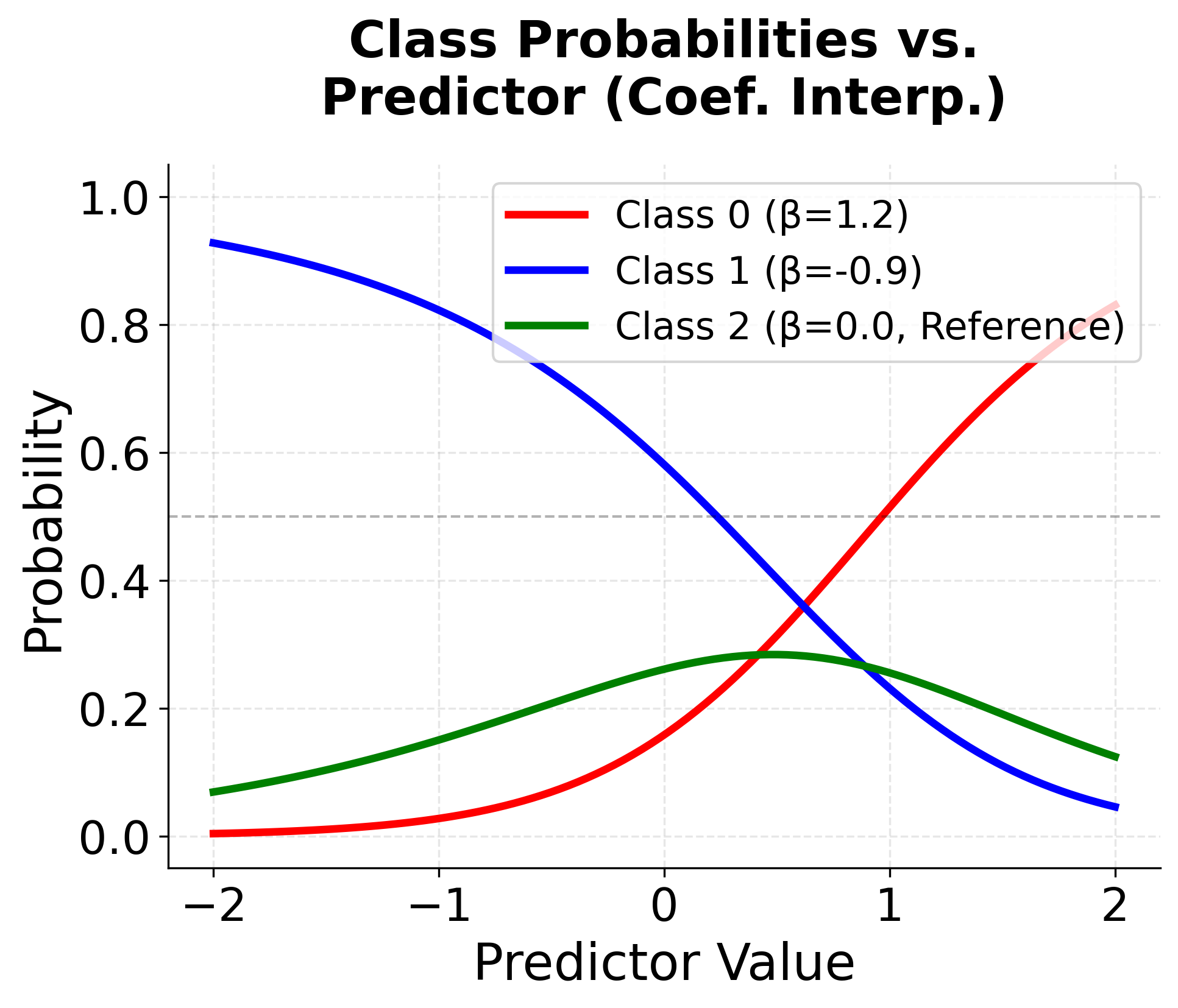
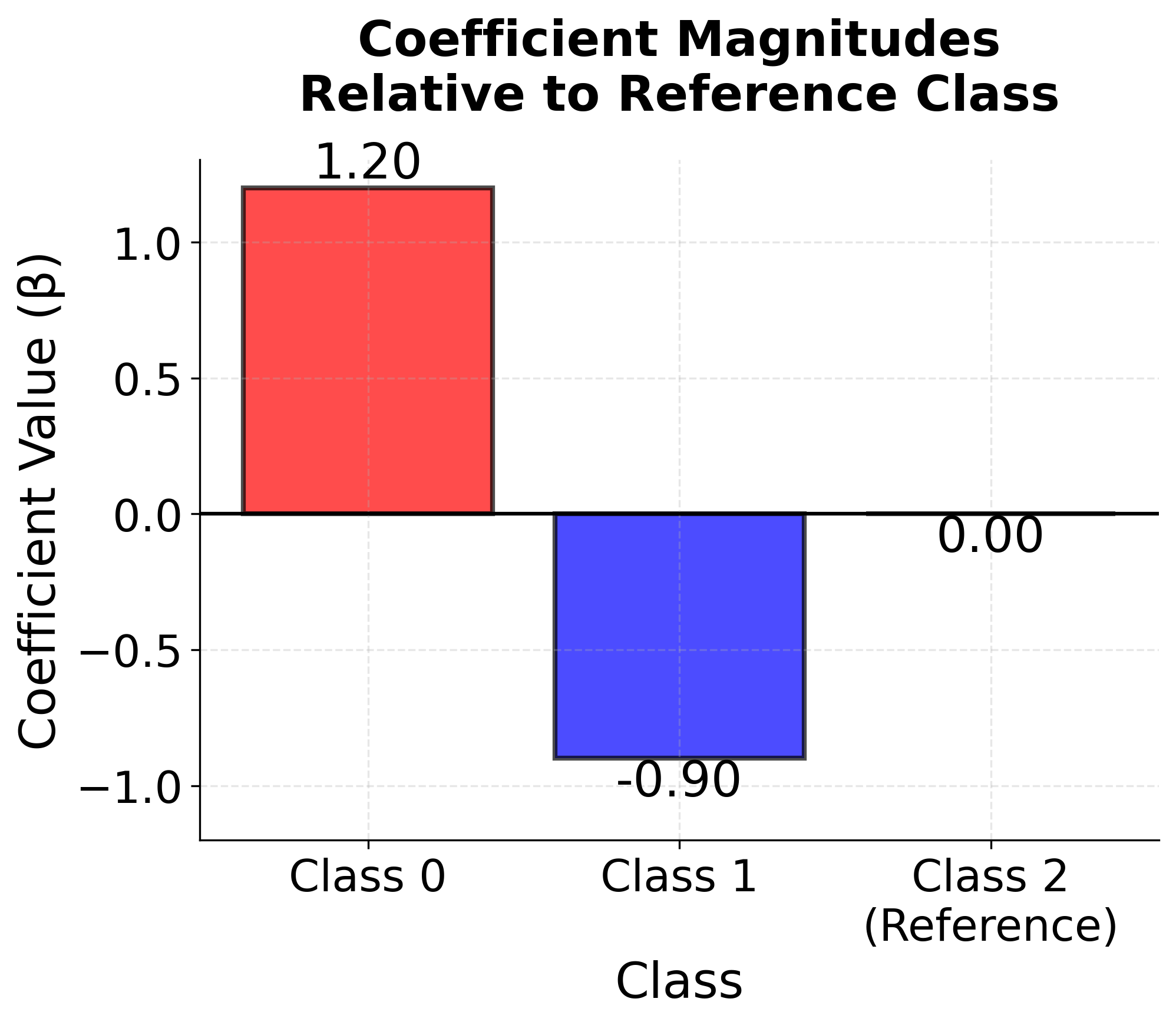
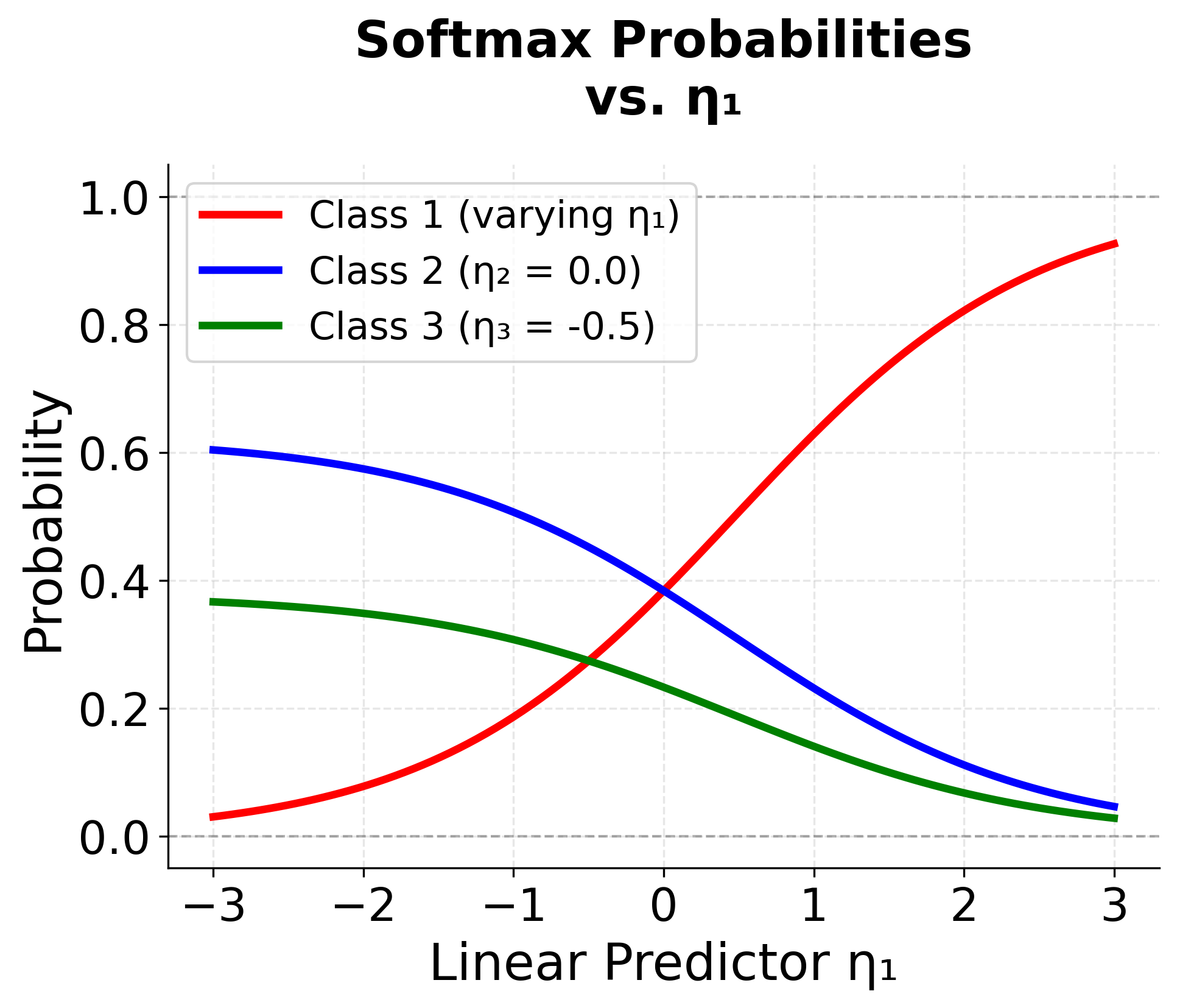
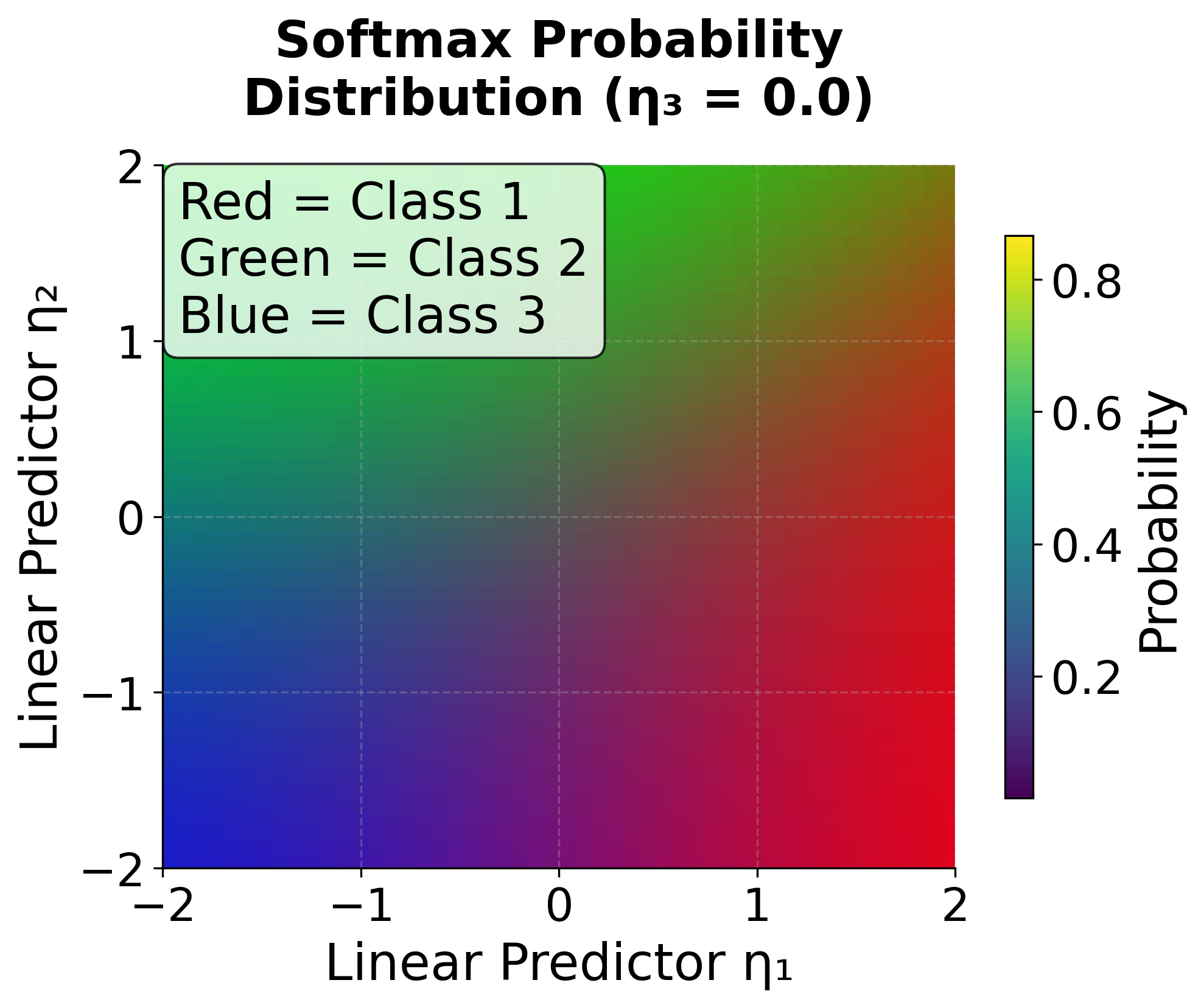
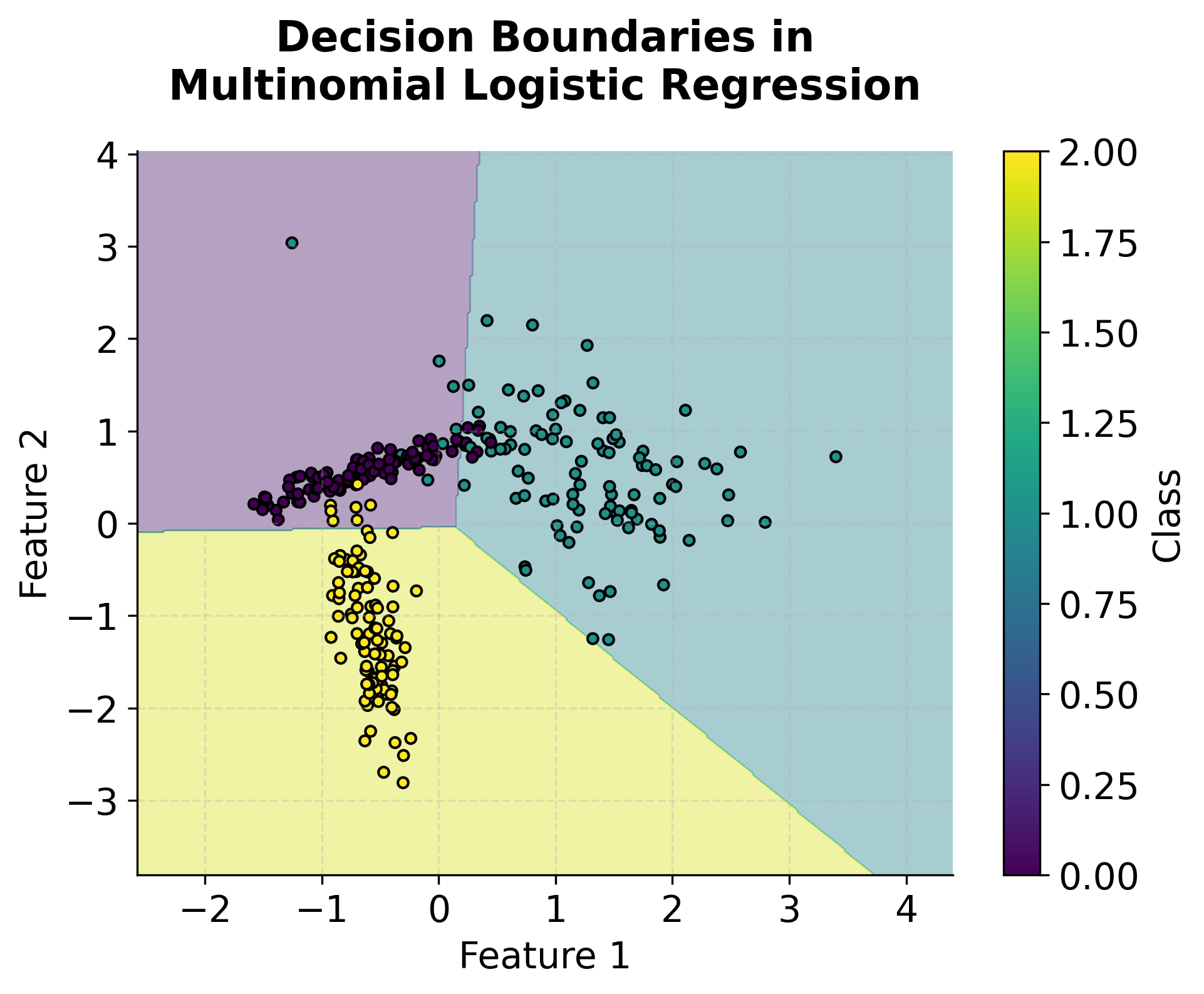
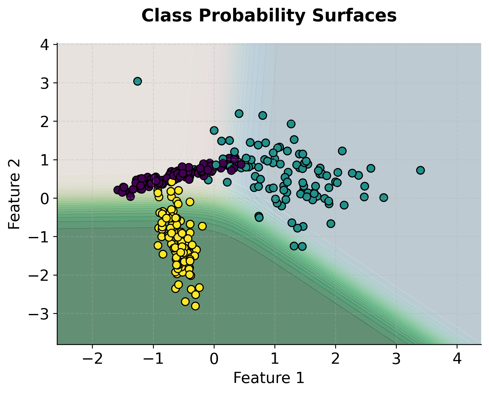
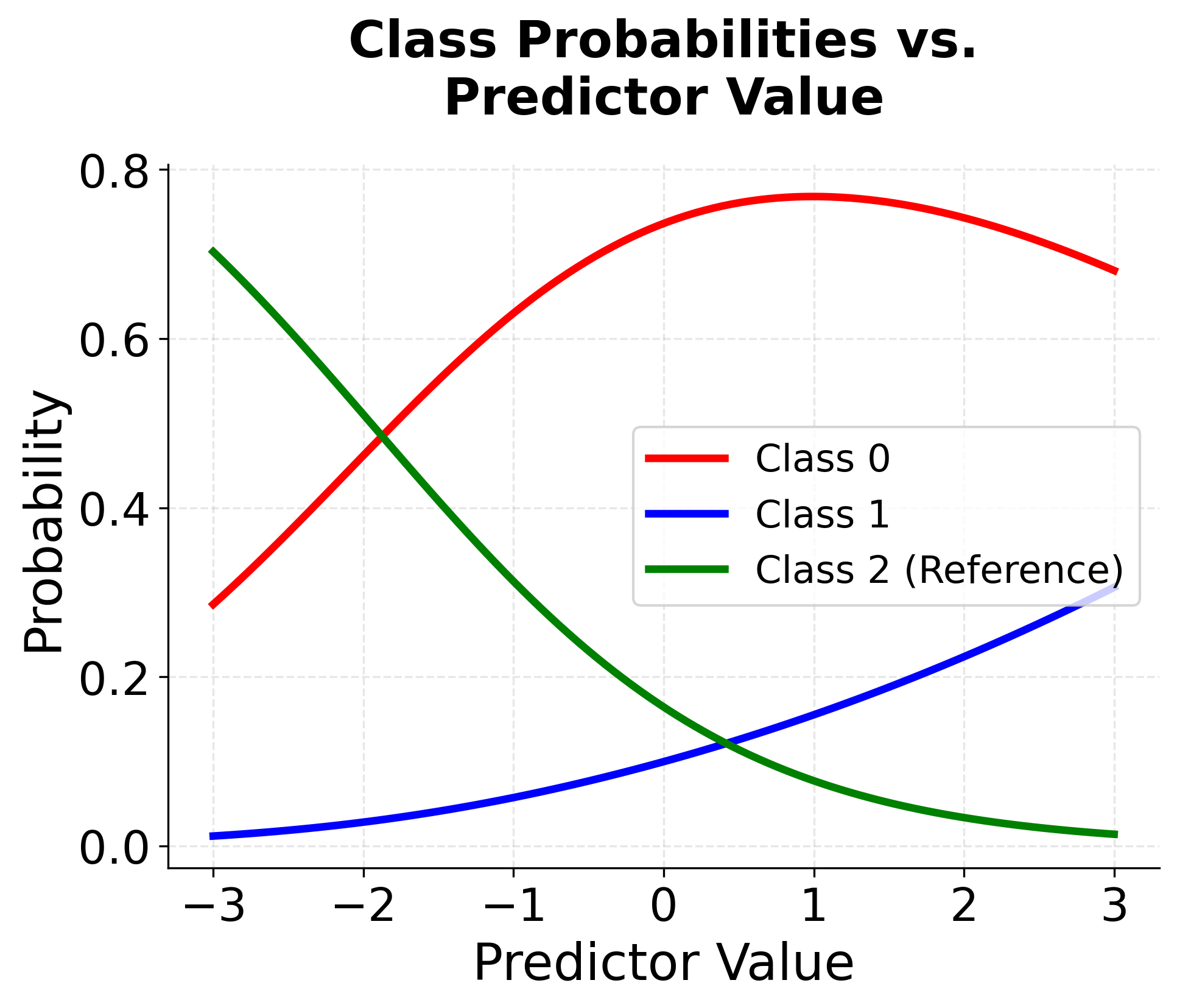
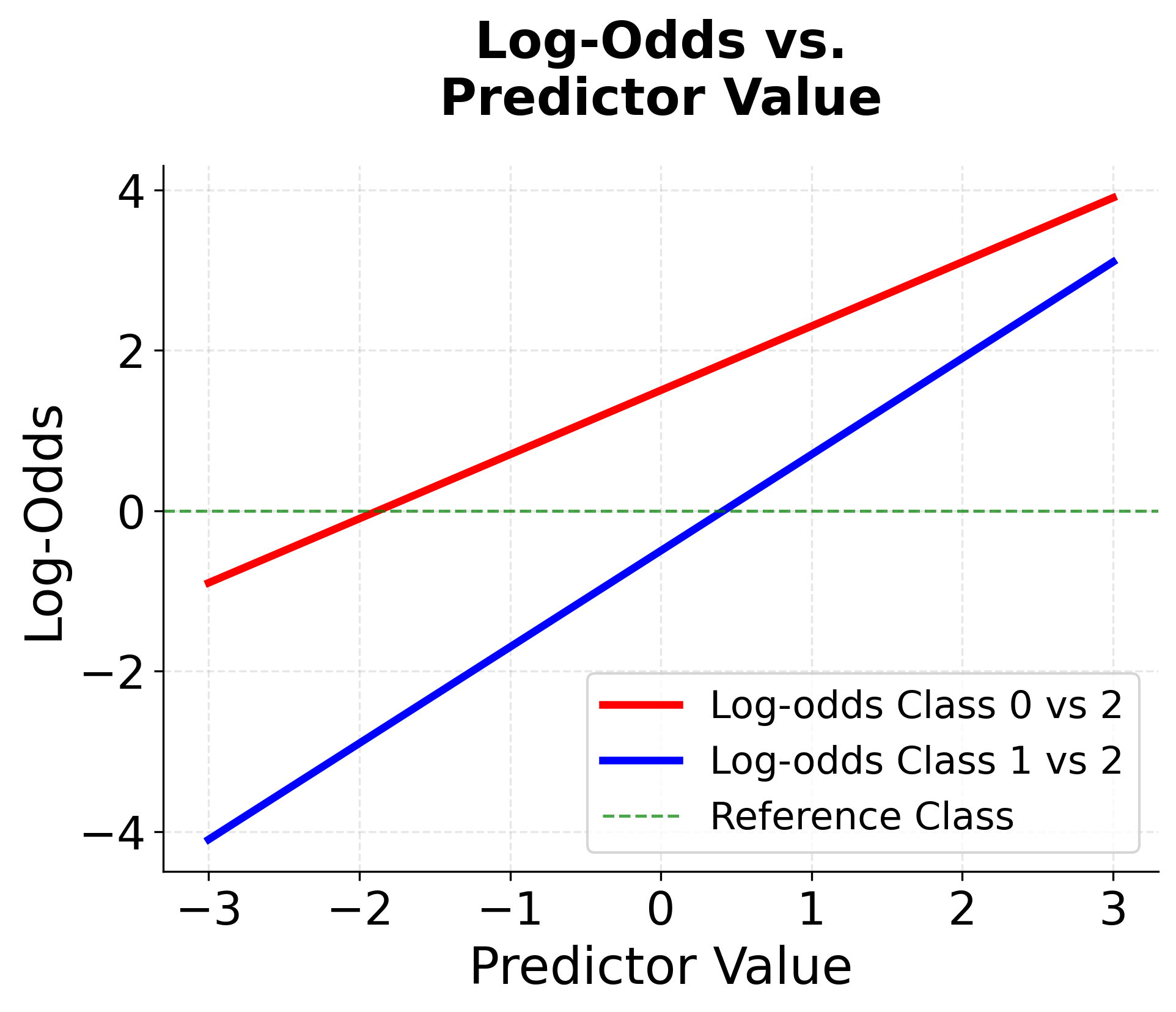
Visualizing Multinomial Logistic Regression

Let's create visualizations to understand how multinomial logistic regression works with different numbers of categories and how the decision boundaries are formed.

Example

Let's work through a concrete example to understand how multinomial logistic regression works with actual numbers. We'll use a simple dataset with two predictor variables and three classes to make the calculations manageable.

Dataset Setup

Suppose we have a dataset with two features (age and income) and three possible outcomes (low, medium, high risk). We'll use "low" as our reference category and calculate the probabilities for "medium" and "high" risk.

Coefficient Estimation

As mentioned in the formula section earlier, the coefficients in multinomial logistic regression are found by solving an optimization problem that maximizes the likelihood of the observed data. In practice, this is done using numerical algorithms such as Newton-Raphson or gradient-based methods, which iteratively adjust the coefficients to best fit the data.

For this example, let's assume we have already obtained the estimated coefficients. We'll now use these given coefficients to demonstrate how to calculate the predicted probabilities for a new observation.

Manual Calculation

Now let's manually calculate the multinomial logistic regression for an observation with age = 25 and income = 30 using these estimated coefficients:

Coefficients for medium vs low (reference):

• $\beta_{\text{medium},0} = 0.5$ (intercept)
• $\beta_{\text{medium},\text{age}} = 0.1$ (age coefficient)
• $\beta_{\text{medium},\text{income}} = -0.05$ (income coefficient)

Coefficients for high vs low (reference):

• $\beta_{\text{high},0} = 1.2$ (intercept)
• $\beta_{\text{high},\text{age}} = 0.15$ (age coefficient)
• $\beta_{\text{high},\text{income}} = -0.08$ (income coefficient)

Step-by-Step Calculation

Step 1: Calculate Linear Predictors

For our observation with age = 25 and income = 30, we calculate the linear predictor for each category:

$\eta_{\text{medium}} = \beta_{\text{medium},0} + \beta_{\text{medium},\text{age}} \times \text{age} + \beta_{\text{medium},\text{income}} \times \text{income}$

where:

• $\eta_{\text{medium}}$ is the linear predictor for the medium risk category (the log-odds of medium risk relative to low risk before normalization)
• $\beta_{\text{medium},0} = 0.5$ is the intercept for medium risk (the baseline log-odds when age and income are both zero)
• $\beta_{\text{medium},\text{age}} = 0.1$ is the age coefficient for medium risk (the change in log-odds for each one-year increase in age)
• $\beta_{\text{medium},\text{income}} = -0.05$ is the income coefficient for medium risk (the change in log-odds for each one-unit increase in income)

Substituting the values:

$\eta_{\text{medium}} = 0.5 + 0.1 \times 25 + (-0.05) \times 30 = 0.5 + 2.5 - 1.5 = 1.5$

Similarly for high risk:

$\eta_{\text{high}} = \beta_{\text{high},0} + \beta_{\text{high},\text{age}} \times \text{age} + \beta_{\text{high},\text{income}} \times \text{income}$

where:

• $\eta_{\text{high}}$ is the linear predictor for the high risk category (the log-odds of high risk relative to low risk before normalization)
• $\beta_{\text{high},0} = 1.2$ is the intercept for high risk (the baseline log-odds when age and income are both zero)
• $\beta_{\text{high},\text{age}} = 0.15$ is the age coefficient for high risk (the change in log-odds for each one-year increase in age)
• $\beta_{\text{high},\text{income}} = -0.08$ is the income coefficient for high risk (the change in log-odds for each one-unit increase in income)

Substituting the values:

$\eta_{\text{high}} = 1.2 + 0.15 \times 25 + (-0.08) \times 30 = 1.2 + 3.75 - 2.4 = 2.55$

For the reference category (low risk):

$\eta_{\text{low}} = 0$

where:

• $\eta_{\text{low}}$ is the linear predictor for the low risk category (set to 0 because low risk is the reference category)

Step 2: Calculate Exponentials

We apply the exponential function to each linear predictor:

$e^{\eta_{\text{medium}}} = e^{1.5} \approx 4.482$

where:

• $e$ is Euler's number (approximately 2.71828)
• $e^{\eta_{\text{medium}}}$ is the exponential of the linear predictor for medium risk (used in the softmax numerator)

$e^{\eta_{\text{high}}} = e^{2.55} \approx 12.807$

where:

• $e^{\eta_{\text{high}}}$ is the exponential of the linear predictor for high risk (used in the softmax numerator)

$e^{\eta_{\text{low}}} = e^{0} = 1.000$

where:

• $e^{\eta_{\text{low}}}$ is the exponential of the linear predictor for low risk (equals 1 because $e^0 = 1$)

Step 3: Calculate Denominator

The denominator of the softmax function is the sum of all exponentials:

$\sum_{k=1}^{K} e^{\eta_k} = e^{\eta_{\text{low}}} + e^{\eta_{\text{medium}}} + e^{\eta_{\text{high}}}$

where:

• $\sum_{k=1}^{K} e^{\eta_k}$ is the sum of exponentials across all $K$ categories (the normalization constant in the softmax function)
• $K = 3$ is the total number of categories (low, medium, high)

Substituting the values:

$\sum_{k=1}^{K} e^{\eta_k} = 1.000 + 4.482 + 12.807 = 18.289$

Step 4: Calculate Probabilities

Using the softmax formula, we calculate the probability for each category:

$P(\text{low}) = \frac{e^{\eta_{\text{low}}}}{\sum_{k=1}^{K} e^{\eta_k}} = \frac{1.000}{18.289} \approx 0.055$

where:

• $P(\text{low})$ is the predicted probability of low risk for this observation (computed by dividing the exponential of the low risk linear predictor by the sum of all exponentials)

$P(\text{medium}) = \frac{e^{\eta_{\text{medium}}}}{\sum_{k=1}^{K} e^{\eta_k}} = \frac{4.482}{18.289} \approx 0.245$

where:

• $P(\text{medium})$ is the predicted probability of medium risk for this observation (computed by dividing the exponential of the medium risk linear predictor by the sum of all exponentials)

$P(\text{high}) = \frac{e^{\eta_{\text{high}}}}{\sum_{k=1}^{K} e^{\eta_k}} = \frac{12.807}{18.289} \approx 0.700$

where:

• $P(\text{high})$ is the predicted probability of high risk for this observation (computed by dividing the exponential of the high risk linear predictor by the sum of all exponentials)

Step 5: Verification

We verify that all probabilities sum to 1, as required by the softmax function:

$P(\text{low}) + P(\text{medium}) + P(\text{high}) = 0.055 + 0.245 + 0.700 = 1.000 \,\checkmark$

Interpretation

The calculations show that for a 25-year-old with income 30, the model predicts:

• 5.5% probability of low risk
• 24.5% probability of medium risk
• 70.0% probability of high risk

The predicted class would be "high" since it has the highest probability. Notice how the probabilities sum to exactly 1, which is a fundamental property of the multinomial logistic regression model.

Implementation in Scikit-learn

Scikit-learn provides an efficient implementation of multinomial logistic regression through the LogisticRegression class. In this section, we'll walk through a complete example using a customer risk classification dataset, demonstrating how to prepare data, train the model, and interpret results.

Data Preparation

First, we'll create our dataset and prepare it for modeling. We'll use age and income as predictors to classify customers into three risk categories:

The LabelEncoder converts the categorical risk levels into numerical values (0, 1, 2), which is required for scikit-learn's implementation. We use stratified splitting to ensure all three risk categories appear in both training and test sets, which is important for reliable evaluation with small datasets.

Model Training

Now let's train the multinomial logistic regression model using the L-BFGS solver, which is well-suited for small to medium-sized datasets:

Model Coefficients

Let's examine the learned coefficients for each class to understand how age and income influence risk classification:

The coefficients reveal how each feature affects the log-odds of each class relative to the reference class (class 0, which corresponds to "high" risk in this encoding). Positive coefficients increase the probability of that class as the feature value increases, while negative coefficients decrease it. For instance, if the age coefficient for the "low" risk class is positive, older customers are more likely to be classified as low risk compared to the reference category. The intercepts represent the baseline log-odds when all features equal zero.

Model Performance

Let's evaluate the model's performance on the test set:

The test accuracy indicates how often the model correctly predicts the risk category. In this case, the model achieves reasonable accuracy despite the very small dataset size. The log loss measures the quality of the probability predictions—lower values indicate better calibrated probabilities, with values closer to 0 being preferable. The small difference between training and test accuracy (if any) suggests the model is not overfitting significantly, which is encouraging given the limited data.

Predictions and Probabilities

Let's examine individual predictions to understand how the model assigns probabilities:

Each prediction shows the complete probability distribution across all three risk categories. The model assigns the observation to the class with the highest probability, but the full distribution provides valuable information about prediction confidence. For example, if one class has a probability of 0.9, the model is very confident, whereas probabilities of 0.4, 0.35, and 0.25 indicate high uncertainty. Notice how the probabilities sum to 1.0 by construction, which is a fundamental property of the softmax function used in multinomial logistic regression.

Classification Report

The classification report provides detailed performance metrics for each class: