InteractiveUMAP: Complete Guide to Uniform Manifold Approximation and Projection for Dimensionality Reduction

UMAP

Uniform Manifold Approximation and Projection (UMAP) is a powerful dimensionality reduction technique that preserves both local and global structure in high-dimensional data. Unlike traditional methods like PCA that focus primarily on global variance, UMAP constructs a representation of the data that maintains the topological structure of the original manifold. This means that points that are close together in the high-dimensional space will remain close in the lower-dimensional projection, while also preserving the overall shape and relationships of the data.

UMAP is particularly valuable because it can handle non-linear relationships that linear methods like PCA cannot capture. While PCA assumes that the data lies on a linear subspace, UMAP makes no such assumption and can discover complex, curved manifolds in the data. This makes it especially useful for visualizing high-dimensional datasets where the underlying structure is non-linear, such as gene expression data, image embeddings, or text representations.

The method works by first constructing a fuzzy simplicial set representation of the data in high dimensions, then finding a low-dimensional representation that has a similar fuzzy simplicial set structure. This approach allows UMAP to capture both local neighborhoods (preserving local structure) and global relationships (preserving global structure) simultaneously, making it particularly effective for both visualization and preprocessing tasks.

Advantages

UMAP offers several key advantages over other dimensionality reduction techniques. First, it preserves both local and global structure, meaning that nearby points in the original space remain close in the reduced space, while the overall shape and relationships of the data are maintained. This dual preservation makes UMAP particularly effective for visualization tasks where we want to understand both fine-grained clusters and broad patterns in the data.

Second, UMAP is computationally efficient and scales well to large datasets. Unlike some other non-linear methods that have quadratic or worse time complexity, UMAP can handle datasets with millions of points in reasonable time. The algorithm uses efficient nearest neighbor search and optimization techniques that make it practical for real-world applications.

Third, UMAP is highly parameterizable, allowing users to tune the balance between local and global structure preservation. By adjusting parameters like n_neighbors and min_dist, we can control whether the algorithm focuses more on preserving local neighborhoods or global structure, making it adaptable to different types of data and analysis goals.

Disadvantages

Despite its strengths, UMAP has several limitations that users should be aware of. The most significant disadvantage is that UMAP is sensitive to its hyperparameters, particularly n_neighbors and min_dist. Choosing inappropriate values can lead to poor results, and the optimal parameters often depend on the specific dataset and analysis goals. This parameter sensitivity can make UMAP less reliable than more robust methods like PCA for certain applications.

Another limitation is that UMAP, like other non-linear dimensionality reduction methods, can be sensitive to noise and outliers in the data. Outliers can significantly affect the construction of the fuzzy simplicial set, potentially distorting the final embedding. This sensitivity to noise means that data preprocessing and outlier detection become more important when using UMAP.

Finally, while UMAP is generally faster than some alternatives like t-SNE, it can still be computationally expensive for very large datasets or when many different parameter combinations need to be tested. The nearest neighbor search, while efficient, still represents a significant computational bottleneck, and the optimization process can be time-consuming for high-dimensional data.

Formula

To understand how UMAP achieves its goal of preserving both local and global structure, we need to explore the mathematical machinery that powers it. The algorithm builds on two key ideas from topology: fuzzy simplicial sets (a way to represent how points relate to each other with partial membership) and Riemannian geometry (which lets us think about distances on curved surfaces). Let's walk through the construction step by step, focusing on the intuition behind each piece.

The Core Challenge

Before diving into formulas, consider the problem UMAP solves. We have high-dimensional data and want to create a low-dimensional representation that preserves important relationships. Linear methods like PCA assume the data lies on a flat hyperplane, but real data often lives on curved manifolds. Imagine a Swiss roll: the data lies on a 2D surface embedded in 3D space. If we simply project it onto a plane, we lose the intrinsic structure. UMAP addresses this by modeling the data as lying on a manifold and preserving the manifold's topology.

The algorithm proceeds in two phases: first, build a rich representation of the high-dimensional structure; second, find a low-dimensional arrangement that matches this structure as closely as possible.

Phase 1: Representing High-Dimensional Structure

Step 1: Computing Local Distances

We start with the basics. For each point $x_i$ in our dataset, we measure how far it is from other points using Euclidean distance:

$d_{ij} = \|x_i - x_j\|_2$

where $d_{ij}$ is the distance between points $x_i$ and $x_j$, and $\|\cdot\|_2$ denotes the Euclidean (L2) norm.

This gives us a distance matrix. UMAP focuses on local neighborhoods because nearby points provide more reliable information about the manifold structure than distant ones.

For each point $x_i$, we identify its $k$ nearest neighbors. These neighbors define a local patch of the manifold around $x_i$. The parameter $k$ (called n_neighbors in practice) controls how many neighbors we consider. A smaller $k$ focuses on very local structure, while a larger $k$ captures more global patterns.

Step 2: Building Fuzzy Membership Strengths

Instead of using a binary neighborhood (where points are either neighbors or not), UMAP assigns a smooth membership strength to each potential neighbor. This membership strength tells us how strongly point $x_j$ belongs to point $x_i$'s local neighborhood.

The membership strength is computed as:

$\mu_{ij} = \exp\left(-\frac{\max(0, d_{ij} - \rho_i)}{\sigma_i}\right)$

where:

• $\mu_{ij}$: Membership strength indicating how strongly point $x_j$ belongs to the neighborhood of point $x_i$
• $\rho_i$: Distance from $x_i$ to its nearest neighbor (acts as a baseline)
• $\sigma_i$: Scaling factor specific to point $x_i$ that controls decay rate
• $d_{ij}$: Euclidean distance between points $x_i$ and $x_j$

Any point closer than the nearest neighbor (when $d_{ij} \leq \rho_i$) gets maximum membership strength of 1.0, since $\max(0, d_{ij} - \rho_i) = 0$ and $\exp(0) = 1$. Beyond the nearest neighbor, the membership strength decays exponentially at a rate controlled by $\sigma_i$.

Why use this exponential decay? Because it creates a smooth, continuous transition from "definitely a neighbor" to "definitely not a neighbor." This smoothness is important for the optimization that comes later.

Finding the Right Scale with $\sigma_i$

The parameter $\sigma_i$ is not chosen arbitrarily. For each point $x_i$, we pick $\sigma_i$ so that the effective number of neighbors equals $k$. Mathematically, we want:

$\sum_{j \neq i} \mu_{ij} = \log_2(k)$

where:

• $\sum_{j \neq i} \mu_{ij}$: Sum of all membership strengths for point $x_i$ (excluding itself)
• $\log_2(k)$: Target sum based on the number of neighbors $k$

Why $\log_2(k)$ instead of just $k$? This comes from information theory and ensures that the fuzzy simplicial set has the right "size" in terms of entropy. We find $\sigma_i$ using binary search: we try different values until the sum of membership strengths equals $\log_2(k)$.

This adaptive scaling is crucial. In dense regions of the data, $\sigma_i$ will be small (neighbors are close, so we don't need to scale distances much). In sparse regions, $\sigma_i$ will be large (neighbors are farther away, so we scale up to maintain connectivity).

Step 3: Creating a Global Graph

Each point $x_i$ now has its own local view of the neighborhood structure, encoded by the membership strengths $\mu_{ij}$. But these local views are asymmetric: point $x_i$ might consider $x_j$ a strong neighbor while $x_j$ considers $x_i$ a weak neighbor (or not at all).

To create a consistent global structure, we symmetrize these relationships using a fuzzy set union:

$\mu_{ij}^{\text{global}} = \mu_{ij} + \mu_{ji} - \mu_{ij} \cdot \mu_{ji}$

where:

• $\mu_{ij}^{\text{global}}$: Symmetrized global membership strength between points $i$ and $j$
• $\mu_{ij}$: Local membership strength from point $i$'s perspective
• $\mu_{ji}$: Local membership strength from point $j$'s perspective

This formula is the probabilistic OR operation for fuzzy sets. It is equivalent to:

$\mu_{ij}^{\text{global}} = 1 - (1 - \mu_{ij})(1 - \mu_{ji})$

In practice, UMAP often uses a simpler approximation:

$\mu_{ij}^{\text{global}} \approx \max(\mu_{ij}, \mu_{ji})$

This approximation says: if either point considers the other a neighbor, preserve that connection in the global graph. The result is a weighted graph where edge weights represent the strength of relationships in the original high-dimensional space.

Phase 2: Finding the Low-Dimensional Embedding

Step 4: Defining Structure in Low Dimensions

Now we have a target: the fuzzy simplicial set $\mu_{ij}^{\text{global}}$ that describes relationships in high dimensions. We need to find low-dimensional coordinates $y_i$ that recreate these relationships as faithfully as possible.

In the low-dimensional space, we compute similar membership strengths. But instead of using exponential decay, UMAP uses a different functional form:

$v_{ij} = \frac{1}{1 + a \cdot \|y_i - y_j\|_2^{2b}}$

where:

• $v_{ij}$: Membership strength between points $i$ and $j$ in the low-dimensional embedding
• $y_i, y_j$: Low-dimensional coordinates of points $i$ and $j$
• $a, b$: Shape parameters that control the distribution (set based on min_dist)

This function is a generalized version of the Cauchy distribution (which t-SNE uses with $b = 1$).

Why a different function in low dimensions? The exponential decay in high dimensions reflects local connectivity on the manifold. In low dimensions, we need a function that allows both tight clusters (when points should be close) and clear separation (when points should be far apart). The form $\frac{1}{1 + a \cdot d^{2b}}$ achieves this balance, where $d = \|y_i - y_j\|_2$ is the Euclidean distance in the low-dimensional space.

The Role of min_dist

The min_dist parameter specifies the minimum distance between points in the low-dimensional embedding. Smaller values allow points to pack tightly (good for revealing fine structure), while larger values spread points out (good for seeing overall organization). The parameters $a$ and $b$ are set to match this desired minimum distance.

Step 5: Optimization via Cross-Entropy

We now have two sets of membership strengths: $\mu_{ij}^{\text{global}}$ (the target from high dimensions) and $v_{ij}$ (the current state in low dimensions). We want to adjust the low-dimensional coordinates $y_i$ to make $v_{ij}$ match $\mu_{ij}^{\text{global}}$ as closely as possible.

UMAP uses cross-entropy as the objective function:

$C = \sum_{i,j} \mu_{ij}^{\text{global}} \log\left(\frac{\mu_{ij}^{\text{global}}}{v_{ij}}\right) + (1 - \mu_{ij}^{\text{global}}) \log\left(\frac{1 - \mu_{ij}^{\text{global}}}{1 - v_{ij}}\right)$

where:

• $C$: Cross-entropy loss to be minimized
• $\mu_{ij}^{\text{global}}$: Target membership strength from high-dimensional space
• $v_{ij}$: Current membership strength in low-dimensional space

Cross-entropy measures the difference between two probability distributions. Here we treat $\mu_{ij}^{\text{global}}$ and $v_{ij}$ as probabilities that points $i$ and $j$ are connected.

The first term, $\mu_{ij}^{\text{global}} \log(\mu_{ij}^{\text{global}} / v_{ij})$, penalizes cases where points should be close (high $\mu_{ij}^{\text{global}}$) but are far apart (low $v_{ij}$). The second term, $(1 - \mu_{ij}^{\text{global}}) \log((1 - \mu_{ij}^{\text{global}}) / (1 - v_{ij}))$, penalizes cases where points should be far apart but are close together.

Minimizing this cross-entropy pulls the low-dimensional structure toward the high-dimensional structure. We use stochastic gradient descent (SGD) to optimize the coordinates $y_i$. At each iteration, we sample pairs of points, compute how the cross-entropy would change if we moved them slightly, and update coordinates to reduce the error.

Why This Construction Works

Let's step back and see the full picture:

1. Local structure preservation: By using nearest neighbors and adaptive scaling ($\sigma_i$), UMAP ensures that local neighborhoods are well-represented.

2. Global structure preservation: By connecting local views into a global fuzzy simplicial set, UMAP maintains large-scale relationships.

3. Flexibility: The low-dimensional membership function and min_dist parameter let us control the final embedding's appearance.

4. Mathematical foundation: The use of fuzzy sets and cross-entropy provides a principled objective function that can be efficiently optimized.

Mathematical Properties

The construction above gives UMAP several important properties:

• Topological preservation: By building a fuzzy simplicial set, UMAP preserves topological features like holes, loops, and connected components. If two clusters are separate in high dimensions, they remain separate in low dimensions.

• Metric structure preservation: UMAP adapts to the local density of the data. In dense regions, it preserves fine details. In sparse regions, it maintains connectivity without distorting distances too much.

• Parameter interpretability: Each parameter has a clear geometric meaning. The n_neighbors parameter controls the size of local neighborhoods (larger values capture more global structure). The min_dist parameter controls how tightly points can cluster in the embedding (smaller values reveal finer details).

• Computational efficiency: By focusing on local neighborhoods and using efficient optimization, UMAP scales to large datasets. The nearest neighbor search is the main computational bottleneck, but this can be accelerated with approximate methods.

Visualizing UMAP

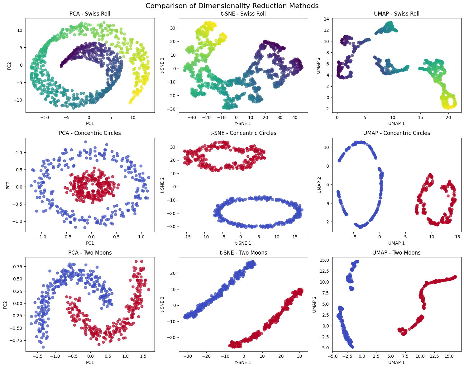
Let's create visualizations that demonstrate how UMAP works and how it compares to other dimensionality reduction methods. We'll start with a simple example using synthetic data to illustrate the key concepts.

Now let's create visualizations comparing the different methods:

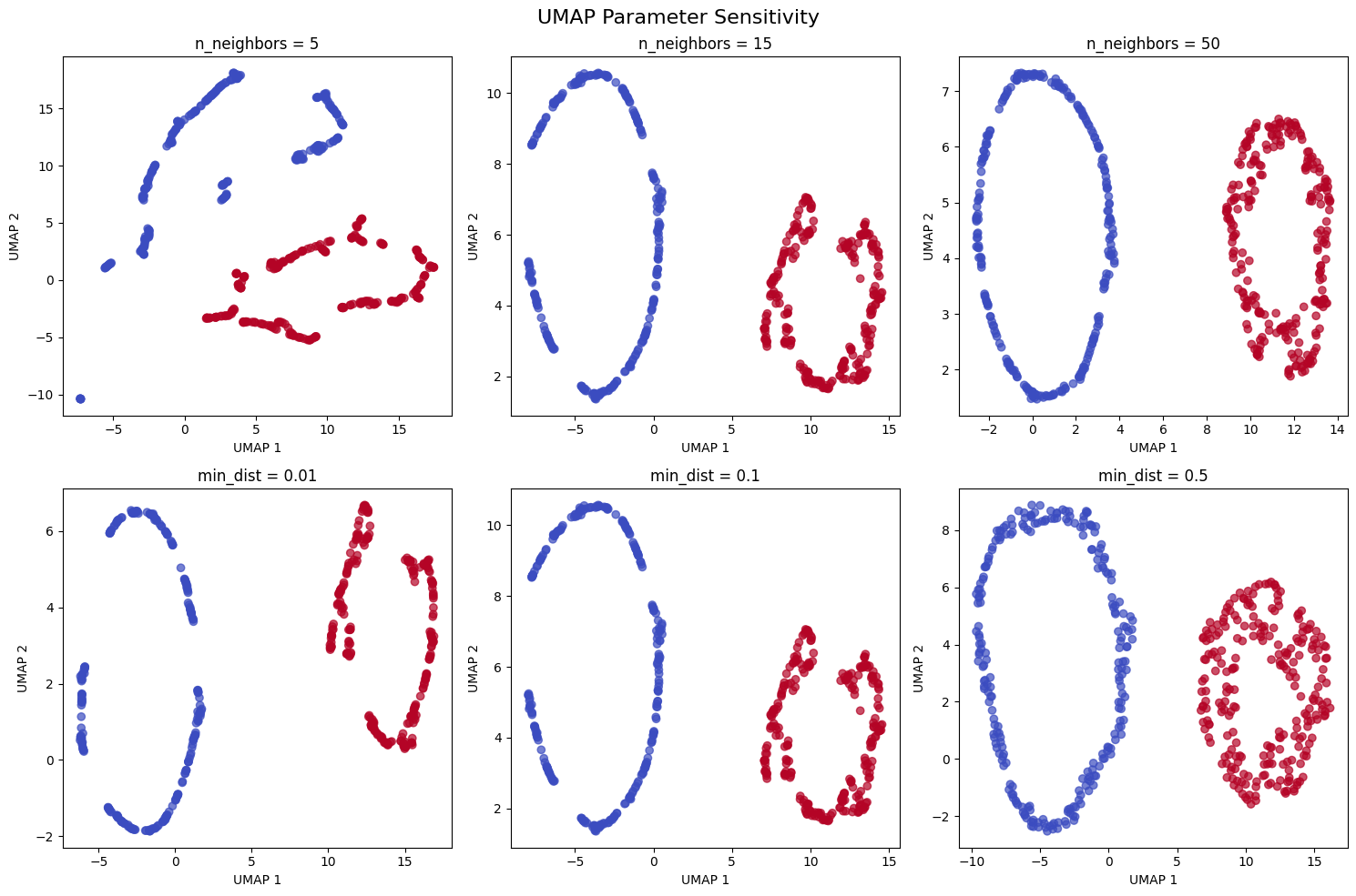
Let's also demonstrate how UMAP parameters affect the results:

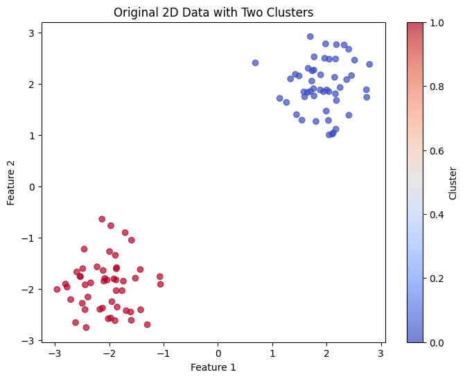
Example

Let's work through a concrete example using a simple 2D dataset to demonstrate how UMAP works step by step. We'll use a dataset with two distinct clusters to make the process clear.

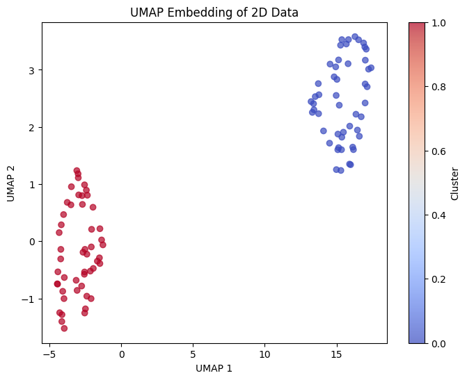
Now let's apply UMAP and examine the results:

Let's also examine the local neighborhood structure that UMAP preserves:

Implementation in Scikit-learn

UMAP is implemented in the umap-learn library, which provides a scikit-learn compatible interface. Let's demonstrate how to use it effectively with a real-world example.

Loading and Preparing Data

We'll use the digits dataset, which contains 8×8 pixel images of handwritten digits (0-9). This is a good example because it has high-dimensional data (64 features) that benefits from dimensionality reduction.

The dataset contains 1,797 samples with 64 features each (representing the 8×8 pixel values). We have 10 classes corresponding to digits 0 through 9.

Preprocessing

UMAP is sensitive to feature scales, so we standardize the features before applying dimensionality reduction.

We've split the data into 80% training (1,437 samples) and 20% test (360 samples) sets. Standardization ensures all features have zero mean and unit variance.

Applying UMAP

Now we apply UMAP to reduce the 64-dimensional data to 2 dimensions for visualization. We set n_neighbors=15 to balance local and global structure, and min_dist=0.1 to allow moderate clustering.

The embedding successfully reduces the dimensionality from 64 to 2 for both training and test sets. Note that we use fit_transform on training data to learn the embedding, then transform on test data to project it into the same embedding space.

Visualizing the Embedding

Let's visualize the 2D UMAP embedding to see how well it separates the different digit classes.

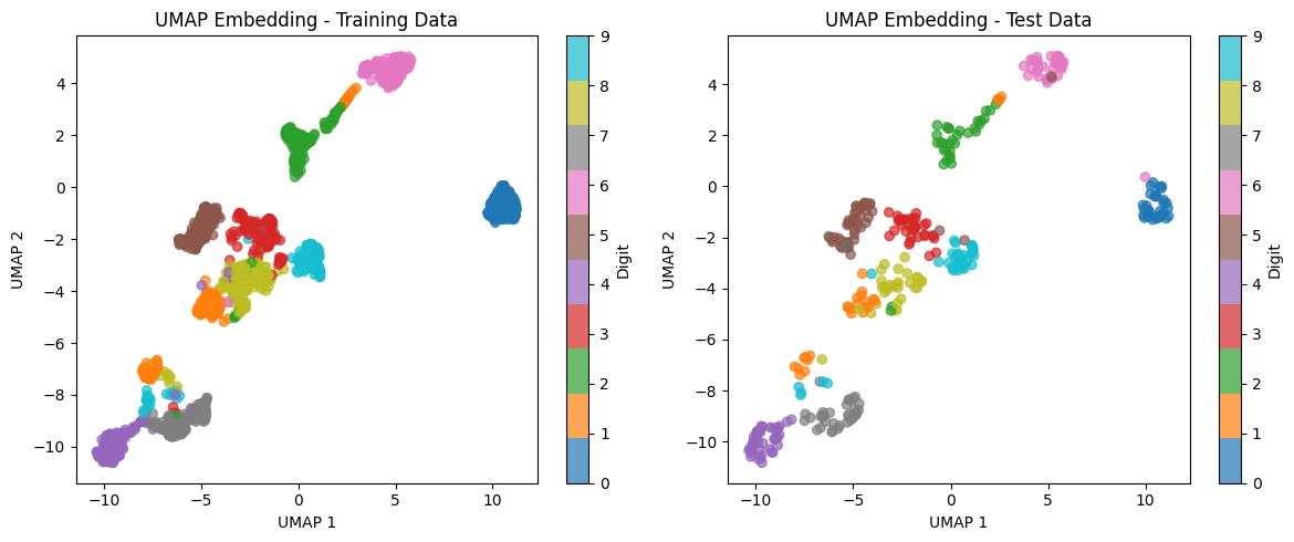
The visualization shows that UMAP successfully groups similar digits together in the 2D space. We can see distinct clusters for each digit class, with some expected overlaps (e.g., between digits that look similar like 3 and 8, or 4 and 9). The test data embedding matches the training data structure, indicating that the learned manifold generalizes well.

Using UMAP for Classification

To demonstrate UMAP's value as a preprocessing step, we'll train a classifier on the reduced 2D representation and compare it to the original 64-dimensional data.

The classifier achieves competitive accuracy even with 97% fewer features. While the original 64-dimensional data provides slightly better accuracy, the 2D UMAP embedding retains most of the discriminative information while being much faster to train and easier to visualize.

The classification report shows per-class performance. Most digits achieve high precision and recall, with the model performing well across all classes. Any confusion between classes reflects the inherent similarity between certain digit shapes in the 2D projection.

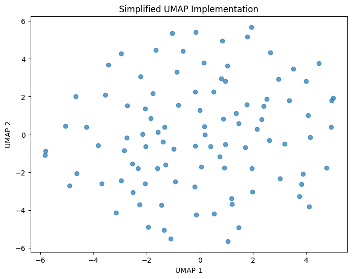
Alternative Implementation

We can also implement a simplified version of UMAP from scratch to better understand the algorithm:

Key Parameters

Below are the main parameters that control how UMAP works and performs. Understanding these parameters helps you tune UMAP for your specific use case.

n_components: Number of dimensions in the low-dimensional embedding (default: 2). Common values are 2 for visualization or 10-50 for preprocessing before other algorithms. Higher values preserve more information but lose visualization benefits.

n_neighbors: Number of nearest neighbors to consider when building the high-dimensional graph (default: 15). This parameter controls the balance between local and global structure:

• Smaller values (5-10): Focus on local structure, revealing fine details and small clusters
• Medium values (15-30): Balance local and global structure, suitable for most applications
• Larger values (50-100): Emphasize global structure, showing broad patterns

min_dist: Minimum distance between points in the low-dimensional embedding (default: 0.1). Controls how tightly points pack together:

• Small values (0.0-0.1): Allow tight clustering, good for finding detailed structure
• Medium values (0.1-0.5): Balance clustering and separation, suitable for most visualizations
• Large values (0.5-0.99): Spread points out more evenly, emphasizing broad organization

metric: Distance metric for computing distances in the high-dimensional space (default: 'euclidean'). Options include 'euclidean', 'manhattan', 'cosine', 'correlation', and many others. Choose based on your data type:

• Euclidean: General-purpose, works well for continuous features
• Cosine: Good for text data or when magnitude doesn't matter
• Manhattan: Robust to outliers in high dimensions

random_state: Seed for reproducibility (default: None). Set to an integer to ensure consistent results across runs.

n_epochs: Number of optimization iterations (default: auto-determined based on dataset size). More epochs improve quality but increase computation time. The default usually works well.

learning_rate: Step size for gradient descent optimization (default: 1.0). Rarely needs adjustment, but lower values (0.1-0.5) can help if the embedding quality is poor.

low_memory: Whether to use a lower memory, but longer-running implementation (default: False). Set to True for very large datasets that don't fit in memory.

Key Methods

The following are the most commonly used methods for interacting with UMAP.

fit(X, y=None): Learns the UMAP embedding from training data X. The optional y parameter can provide supervised information to guide the embedding.

fit_transform(X, y=None): Fits the model and returns the transformed data in one step. Use this for the initial embedding of your training data.

transform(X): Projects new data into the existing embedding space. Use this for test data or new observations after fitting on training data. Note that transform may be less accurate than the original embedding.

inverse_transform(X_embedded): Attempts to reconstruct the original high-dimensional data from the low-dimensional embedding. This is approximate and works better for higher-dimensional embeddings.

Practical Applications

When to Use UMAP

UMAP is particularly valuable when working with high-dimensional data that contains non-linear structure. In bioinformatics and genomics, UMAP excels at visualizing gene expression data from single-cell RNA sequencing experiments. These datasets typically contain thousands of genes (features) measured across thousands of cells, with complex relationships that form curved manifolds in high-dimensional space. UMAP's ability to preserve both local neighborhoods (grouping similar cells) and global structure (maintaining relationships between cell types) makes it effective for identifying cell populations, developmental trajectories, and disease states that might be missed by linear methods.

For machine learning practitioners, UMAP serves as a preprocessing step before classification or clustering when dealing with high-dimensional embeddings. In computer vision, image representations from deep neural networks often capture semantic relationships that lie on non-linear manifolds. UMAP can reduce these embeddings from hundreds or thousands of dimensions to a manageable size while preserving the neighborhood structure that indicates visual similarity. Similarly, in natural language processing, word embeddings and document representations benefit from UMAP's ability to maintain both local semantic relationships and broader topical structure.

UMAP is also useful in exploratory data analysis when you need to understand the structure of your data before modeling. The 2D or 3D visualizations it produces can reveal clusters, outliers, and relationships that inform feature engineering, model selection, and data quality assessment. However, UMAP is less suitable when your data truly lies on a linear subspace, when you need deterministic results without parameter tuning, or when computational resources are severely limited. In these cases, PCA may be more appropriate despite its linear assumptions.

Best Practices

To achieve optimal results with UMAP, start with the default parameters (n_neighbors=15, min_dist=0.1) and adjust based on your specific needs. For visualization tasks, keep n_components=2 or n_components=3 to enable plotting. For preprocessing before other algorithms, use higher dimensions (10-50) to retain more information while still reducing computational cost. When your dataset is small (fewer than 1,000 samples), reduce n_neighbors to 5-10 to avoid forcing the algorithm to consider too many neighbors relative to the dataset size. For large datasets (over 10,000 samples), you can increase n_neighbors to 30-50 to capture more global structure.

The min_dist parameter controls the visual appearance of your embedding. Smaller values (0.0-0.05) create tight, distinct clusters that emphasize fine-grained structure, which works well when you expect many small groups. Larger values (0.3-0.5) spread points out more evenly, making it easier to see the overall organization at the cost of losing some local detail. For exploratory analysis, try multiple min_dist values to understand your data from different perspectives. Set random_state to an integer for reproducibility, as UMAP uses stochastic optimization that produces different results across runs.

Evaluate your UMAP embeddings using multiple approaches rather than relying on a single metric. Quantitatively, measure how well the embedding preserves local neighborhoods by comparing nearest neighbors in the original space versus the embedded space. Visually, check whether the embedding reveals meaningful structure by coloring points according to known labels or metadata. If you see unexpected patterns or poor separation, try adjusting n_neighbors or min_dist, or verify that your preprocessing was appropriate. Remember that UMAP makes tradeoffs to compress high-dimensional data into low dimensions, so perfect preservation is impossible.

Data Requirements and Preprocessing

UMAP requires numerical feature data and is sensitive to feature scales because it computes distances in the original high-dimensional space. Before applying UMAP, standardize your features using z-score normalization (zero mean, unit variance) to ensure that all features contribute equally to distance calculations. Features measured in different units or with vastly different ranges will otherwise dominate the embedding, leading to distorted results. For example, if one feature ranges from 0-1000 while another ranges from 0-1, the larger-scale feature will disproportionately influence neighborhood calculations.

When working with very high-dimensional data (thousands of features), consider applying PCA as a preprocessing step to reduce dimensionality to a few hundred components before using UMAP. This approach reduces computational cost, removes noise, and often improves UMAP's ability to find meaningful structure. However, avoid reducing to very few PCA components (fewer than 10-20), as this may remove non-linear relationships that UMAP could otherwise discover. The combination of PCA for noise reduction and linear structure removal, followed by UMAP for non-linear manifold learning, often produces better results than either method alone.

Handle missing values before applying UMAP, as the algorithm requires complete data for distance calculations. Either impute missing values using appropriate methods for your domain, or remove samples with missing data if your dataset is large enough. Similarly, identify and handle outliers carefully. Extreme outliers can distort distance calculations and affect the fuzzy simplicial set construction, potentially pulling the embedding in misleading directions. Consider whether outliers represent meaningful rare cases or data quality issues, and treat them accordingly.

Common Pitfalls

One frequent mistake is using UMAP without standardizing features, which leads to embeddings dominated by high-variance or large-scale features. This is particularly problematic when features have different units (e.g., mixing counts, proportions, and measurements in different scales). The resulting visualization may appear to show clear structure, but the patterns reflect scale differences rather than meaningful relationships. Check your feature scales before running UMAP, and standardize unless you have a specific reason not to (such as when all features are already comparable, like pixel values from images).

Another common issue is over-interpreting distances in UMAP embeddings. While UMAP preserves local neighborhoods well, global distances can be distorted, and the distance between clusters in the 2D embedding does not necessarily reflect their true separation in the original space. Two clusters that appear far apart in the UMAP visualization might actually be close in the high-dimensional space, or vice versa. Use UMAP primarily for understanding local structure and overall topology, not for precise distance measurements. If global distances matter for your analysis, consider alternative methods or validate UMAP results with distance calculations in the original space.

Failing to experiment with different parameter values is another pitfall. Many users stick with default parameters even when they produce suboptimal results for their specific data. If your embedding looks overly compressed or overly dispersed, lacks clear structure when you expect to see it, or shows unexpected patterns, try adjusting n_neighbors and min_dist. Start by varying n_neighbors across a range (5, 15, 30, 50) to see how the balance between local and global structure changes. Similarly, try several min_dist values (0.0, 0.1, 0.3) to find the level of compactness that best reveals your data's structure. Document which parameters work best for your use case to guide future analyses.

Computational Considerations

UMAP's computational complexity depends primarily on the nearest neighbor search and the optimization process. For datasets with tens of thousands of points, UMAP typically completes in minutes on modern hardware. The nearest neighbor search scales approximately as O(n log n) when using efficient tree-based or approximate methods, while the optimization phase scales roughly linearly with the number of points and edges in the graph. Memory usage is dominated by storing the nearest neighbor graph, which requires O(n × n_neighbors) space.

For large datasets (over 100,000 points), consider strategies to reduce computational cost. Reduce n_neighbors from the default 15 to 10 or even 5, which decreases both the graph construction time and memory requirements. Use approximate nearest neighbor methods by setting metric='euclidean' and ensuring your implementation uses efficient approximations (most modern UMAP implementations do this automatically). For extremely large datasets (millions of points), consider subsampling to a representative subset, applying UMAP to learn the embedding, and then projecting the remaining points using the transform method. This approach trades some accuracy for substantial speed improvements.

UMAP benefits from parallelization during the nearest neighbor search phase when multiple CPU cores are available. Most implementations automatically use multiple cores for this step. However, setting random_state disables some parallelization to ensure reproducibility, which can slow down computation. For production use cases where speed matters more than exact reproducibility, consider omitting random_state or running multiple trials in parallel with different random seeds to verify stability. For deployment scenarios requiring fast inference on new data points, precompute the UMAP embedding on a reference dataset and use the transform method for new points, though be aware that transformed points may have lower quality embeddings than the original fitted data.

Performance and Deployment Considerations

Evaluating UMAP embeddings requires multiple complementary approaches because there is no single metric that captures all aspects of quality. Quantitatively, measure neighborhood preservation by computing the overlap between k-nearest neighbors in the original space and the embedded space. A preservation rate above 0.7 indicates that the embedding maintains most local structure, while rates below 0.5 suggest that significant information has been lost. You can also measure how well the embedding preserves pairwise distances by comparing distance rankings before and after dimensionality reduction using Spearman correlation.

Visual inspection remains important despite quantitative metrics. Color points in the embedding according to known labels, metadata, or features to verify that meaningful patterns emerge. Clusters of the same color indicate that UMAP successfully grouped similar items. Check for gradients or continuous transitions in the embedding when you expect them (e.g., developmental trajectories in biological data). Be cautious about finding spurious patterns—UMAP can create apparent structure even in random data, so validate findings against domain knowledge or external data.

When deploying UMAP in production systems, consider the computational cost of fitting versus transforming. Fitting UMAP requires significant computation and should be done on a representative training set. Once fitted, the model can transform new points using the transform method, which is faster but produces lower-quality embeddings than the original fit_transform. For applications requiring high-quality embeddings of new data, periodically refit UMAP on an updated reference dataset that includes recent samples. Monitor the neighborhood preservation metric over time to detect when the embedding quality degrades, which may indicate data drift or the need to update the reference embedding. Store UMAP models along with the preprocessing pipeline (standardization parameters, PCA components if used) to ensure consistent transformations of new data.

Summary

UMAP advances dimensionality reduction by combining local structure preservation with global structure preservation. The method's foundation in fuzzy simplicial sets and Riemannian geometry provides a mathematically rigorous approach to manifold learning that scales well to large datasets while maintaining interpretable parameters.

The algorithm's strength lies in revealing non-linear relationships that linear methods like PCA cannot capture. This capability makes UMAP valuable for visualization and preprocessing in fields where data structure is inherently non-linear, such as genomics, computer vision, and natural language processing. The balance between local and global preservation can be tuned through the n_neighbors and min_dist parameters to match specific analysis goals.

The main tradeoff involves parameter sensitivity. While PCA has no parameters to tune, UMAP requires thoughtful selection of n_neighbors (which controls the locality of the embedding) and min_dist (which controls point spacing). Feature standardization is recommended when scales differ across dimensions. Despite these requirements, UMAP provides a flexible approach to understanding high-dimensional data that complements traditional linear methods.