
A comprehensive guide to multiple linear regression, including mathematical foundations, intuitive explanations, worked examples, and Python implementation. Learn how to fit, interpret, and evaluate multiple linear regression models with real-world applications.
This article is part of the free-to-read Machine Learning from Scratch
Choose your expertise level to adjust how many terms are explained. Beginners see more tooltips, experts see fewer to maintain reading flow. Hover over underlined terms for instant definitions.
Multiple Linear Regression
Multiple linear regression extends simple linear regression to model relationships between multiple predictor variables and a single target variable. While simple linear regression fits a line through data points, multiple linear regression fits a hyperplane—a flat surface in higher-dimensional space—that captures how multiple features collectively influence the target variable.
The key insight of multiple linear regression is that real-world outcomes are typically influenced by multiple factors simultaneously. House prices depend on size, location, age, and neighborhood characteristics. Sales performance reflects advertising spend, seasonality, competitor pricing, and economic conditions. By incorporating multiple relevant features, we can capture these complex relationships and make more accurate predictions than using single variables in isolation.
Multiple linear regression assumes that the relationship between features and the target is linear and additive. This means each feature contributes independently to the prediction, and the effect of changing one feature by a unit remains constant regardless of other feature values. While this assumption may seem restrictive, linear models often perform well in practice and provide interpretable results that are valuable for understanding and explaining relationships in data.
Advantages
Multiple linear regression offers several key advantages for predictive modeling and statistical analysis. The method is highly interpretable—each coefficient directly shows how much the target variable changes when the corresponding feature increases by one unit, holding all other features constant. This makes it excellent for understanding relationships in data and explaining results to stakeholders.
The method is computationally efficient and typically doesn't require extensive hyperparameter tuning. Unlike many machine learning algorithms, you generally don't need to worry about learning rates, regularization parameters, or complex optimization settings. The closed-form solution provides consistent, optimal results.
Additionally, multiple linear regression provides a solid foundation for understanding more advanced techniques. Once you grasp the concepts of feature interactions, regularization, and model evaluation in this context, you'll find it much easier to understand more sophisticated methods like polynomial regression, ridge regression, or even neural networks.
Disadvantages
Despite its strengths, multiple linear regression has several limitations that should be considered. The most significant constraint is the linearity assumption—the model assumes that relationships between features and the target are linear and additive. In reality, many relationships are non-linear, and features often interact with each other in complex ways that a simple linear model cannot capture.
The method is sensitive to outliers and can be heavily influenced by extreme values in the data. A single outlier can significantly change coefficient estimates and predictions. Additionally, when features are highly correlated (multicollinearity), coefficient estimates can become unstable and difficult to interpret, though the model itself doesn't require features to be independent.
Another limitation is that the model doesn't automatically handle feature selection—it will use all features provided, even if some are irrelevant or redundant. This can lead to overfitting, especially when you have many features relative to your sample size. You may need to use additional techniques like stepwise selection or regularization to address this issue.
Note: Multiple linear regression does not assume that features are independent of each other. The model can handle correlated features effectively. However, when features are highly correlated (multicollinearity), the coefficient estimates become unstable and difficult to interpret because the model cannot distinguish between the individual effects of highly correlated features. This is a practical concern rather than a theoretical assumption violation.
Mathematical Foundation
Multiple linear regression extends the simple linear regression model to incorporate multiple predictor variables. The mathematical foundation builds upon the principles of ordinary least squares (OLS) estimation, which is covered in detail in the dedicated OLS chapter.
Model Specification
The multiple linear regression model can be written as:
where:
- : observed value of the target variable for the -th observation
- : intercept (bias term) - the predicted value of when all features equal zero
- : coefficients (slopes) for each feature, representing the partial effect of each feature
- : values of the features for the -th observation
- : error term (residual) - the difference between the actual and predicted values
The key insight is that each coefficient represents the partial effect of feature on the target variable, holding all other features constant. This is the fundamental difference from simple linear regression, where we only consider one feature at a time.
Matrix Notation
When working with observations and features, the model can be written compactly using matrix notation:
where:
- : vector containing all observed target values
- : design matrix containing all feature values with a column of ones for the intercept
- : vector of coefficients (including intercept)
- : vector of error terms (residuals)
The design matrix has the structure:
The first column of ones enables estimation of the intercept term, while subsequent columns contain the feature values for each observation.
Coefficient Estimation
The coefficients in multiple linear regression are estimated using the Ordinary Least Squares (OLS) method, which finds the values of that minimize the sum of squared differences between observed and predicted values.
The OLS solution is given by the closed-form formula:
where:
- : estimated coefficient vector (including intercept)
- : matrix of feature cross-products
- : inverse of the cross-product matrix
- : vector of feature-target covariances
For a detailed mathematical derivation of this formula, including the normal equations and computational considerations, see the dedicated OLS chapter.
Key Properties
The OLS solution has several important properties:
- Unbiased: The estimates are unbiased under standard regression assumptions
- Efficient: Among all unbiased linear estimators, OLS has the smallest variance
- Consistent: As sample size increases, the estimates converge to the true values
While the closed-form solution is mathematically elegant, computing can be problematic when:
- The matrix is nearly singular (ill-conditioned) due to multicollinearity
- You have more features than observations ()
- The dataset is very large
In these cases, numerical methods like QR decomposition, SVD, or gradient descent are preferred for stability and efficiency.
Understanding Multiple Linear Regression Through Visualization
The mathematical components of multiple linear regression can be visualized to make the abstract concepts more concrete. This visualization shows how the matrix operations work together to find the optimal coefficients for multiple features.
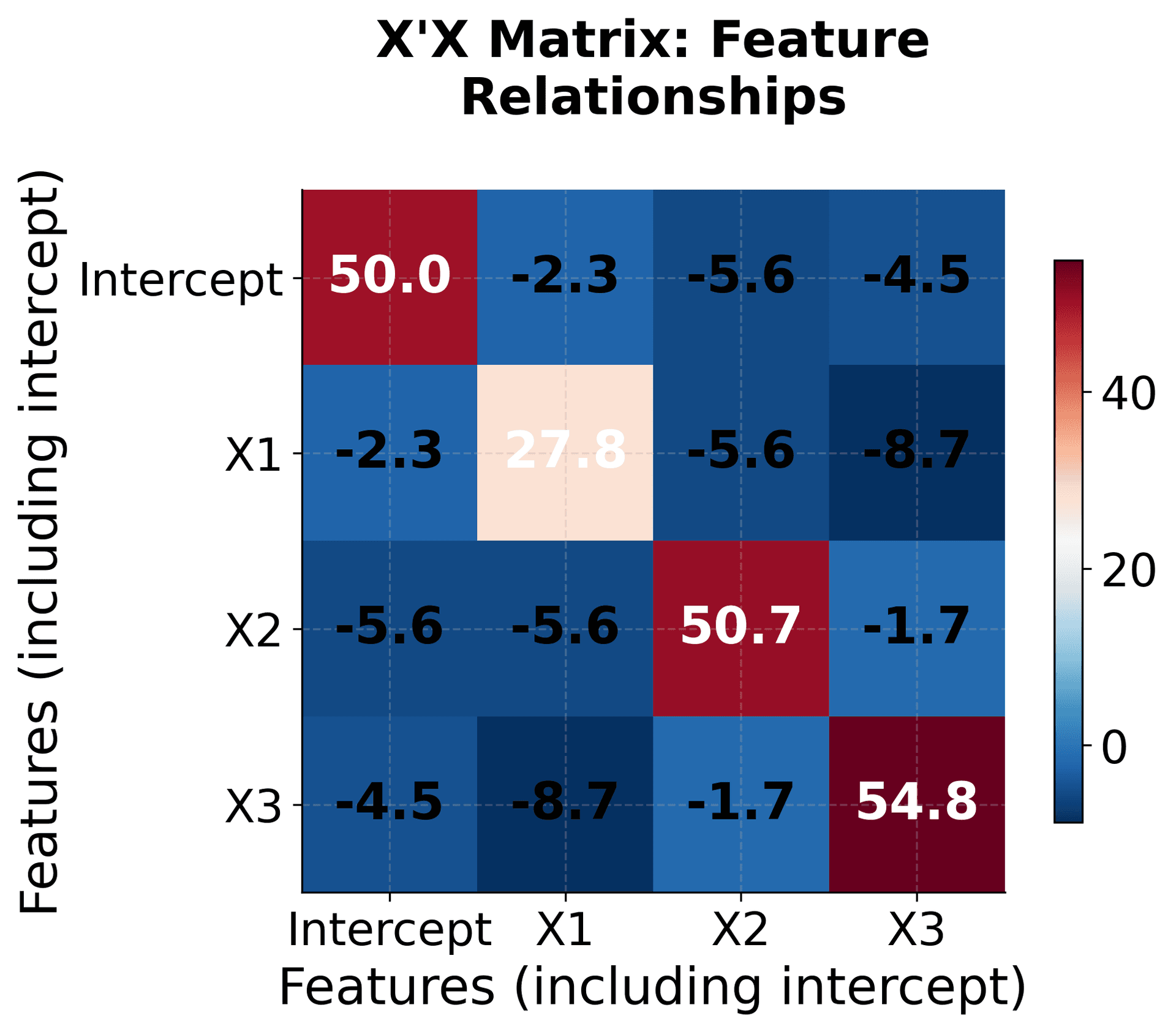
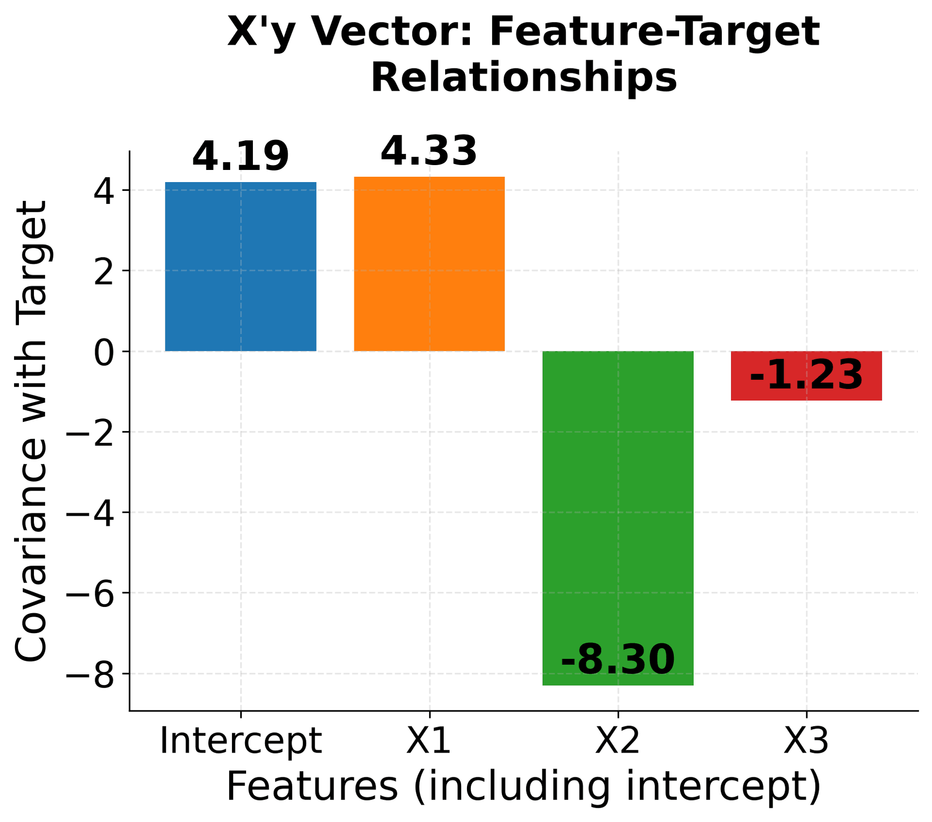
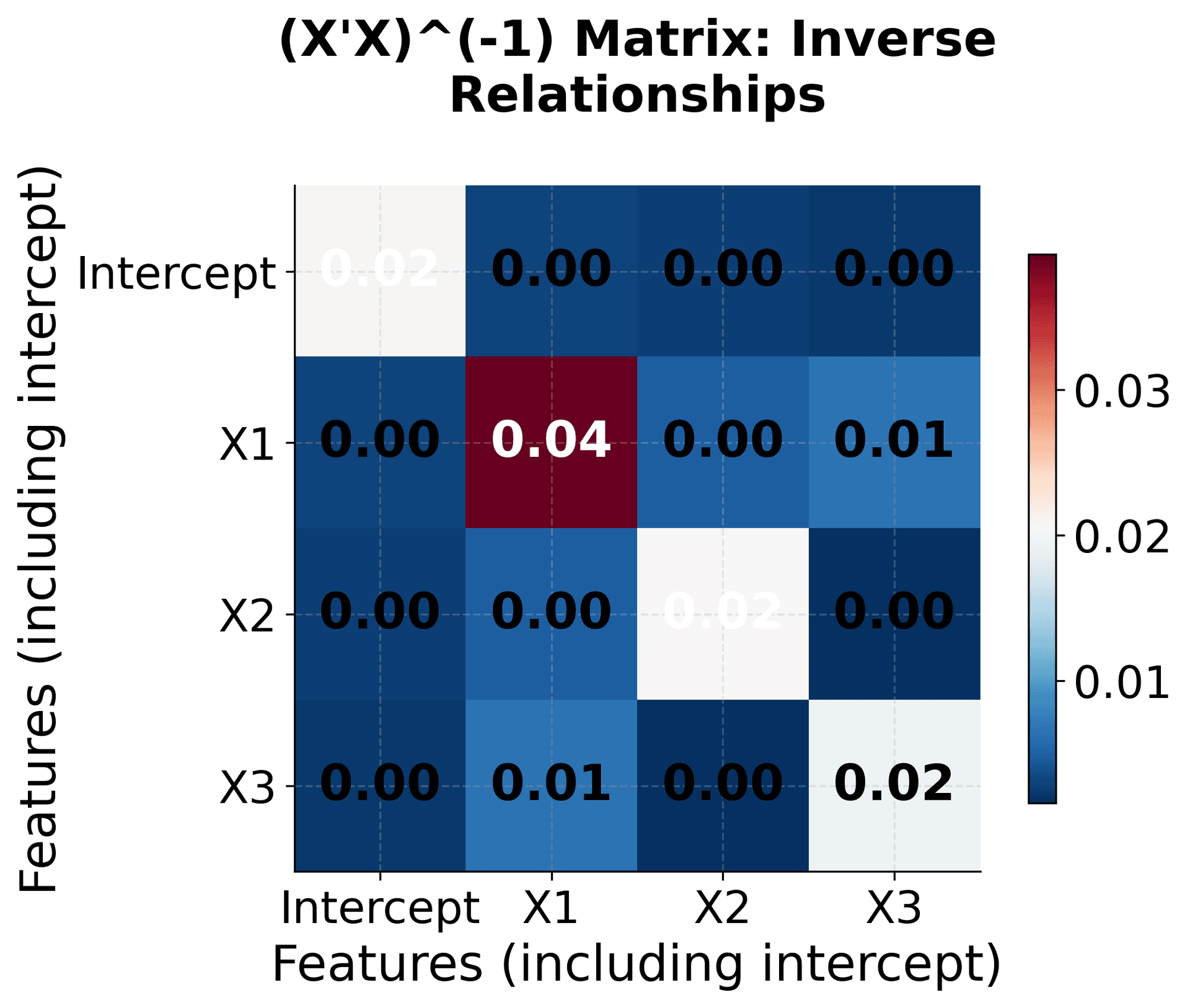
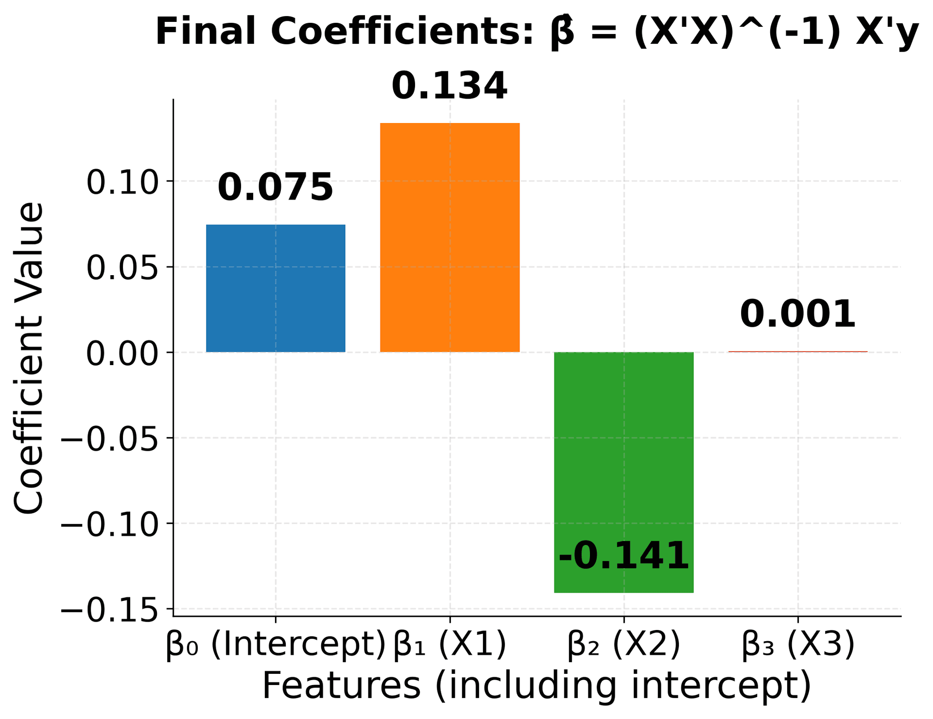
This visualization breaks down the multiple linear regression solution into its component parts, making the abstract matrix operations concrete and understandable. The X'X matrix shows how features relate to each other, X'y captures feature-target relationships, and the inverse operation transforms these into optimal coefficients.
Visualizing Multiple Linear Regression
The best way to understand multiple linear regression is through visualization. Since we can only directly visualize up to three dimensions, we'll focus on the case with two features, which creates a 3D visualization where we can see how the model fits a plane through the data points.
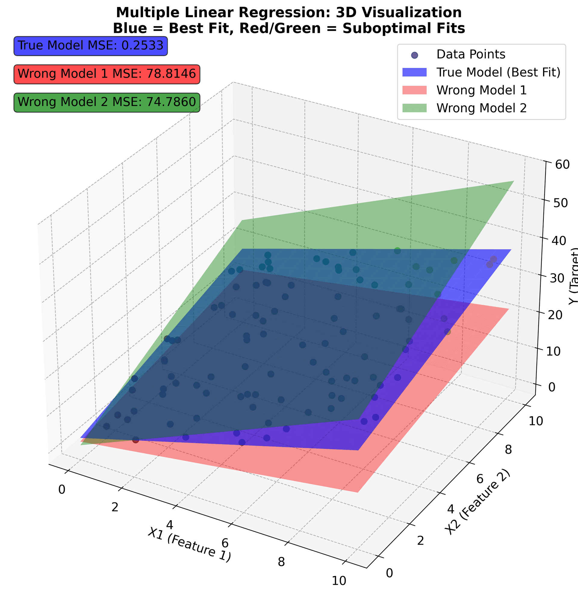
This visualization shows the fundamental concept of multiple linear regression in three dimensions. The colored dots represent your actual data points, where each point's position is determined by its values for X1, X2, and Y. The color intensity reflects the Y value, helping you see the pattern in your data.
The blue surface represents the optimal hyperplane that best fits your data. This plane is defined by the equation , which accurately captures the underlying relationship between your features and target variable. The red and green surfaces show alternative models with different coefficients that don't fit the data as well.
The Mean Squared Error (MSE) values displayed in the corner boxes quantify how well each model performs. The true model has the lowest MSE (0.25), confirming that it provides the best fit. The other models have higher MSE values, indicating they make larger prediction errors.
Key insights from this visualization:
- Hyperplane fitting: Multiple linear regression finds the flat surface that best represents the relationship between your features and target
- Error minimization: The optimal plane minimizes the sum of squared vertical distances from data points to the surface
- Coefficient interpretation: Each coefficient determines the slope of the plane in the direction of its corresponding feature
- Model comparison: MSE provides a quantitative way to compare different models and select the best one
When you have more than two features, you work in higher-dimensional spaces where hyperplanes cannot be directly visualized. However, the mathematical principles remain identical—you're still finding the flat surface that best fits your data, just in a space with more dimensions. The OLS formula works the same way regardless of how many features you have.
Understanding Coefficient Interpretation
One of the most important aspects of multiple linear regression is understanding what the coefficients mean in practical terms. Let's see how coefficients represent the partial effect of each feature while holding all other features constant.
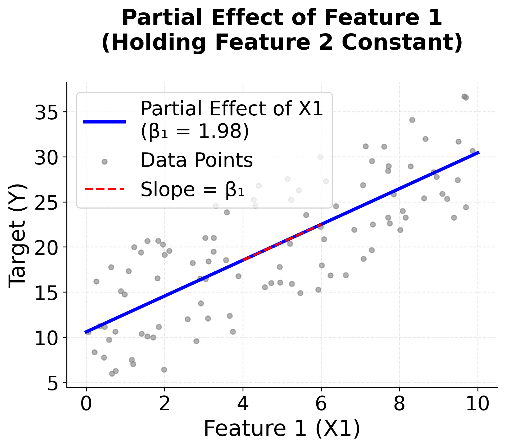
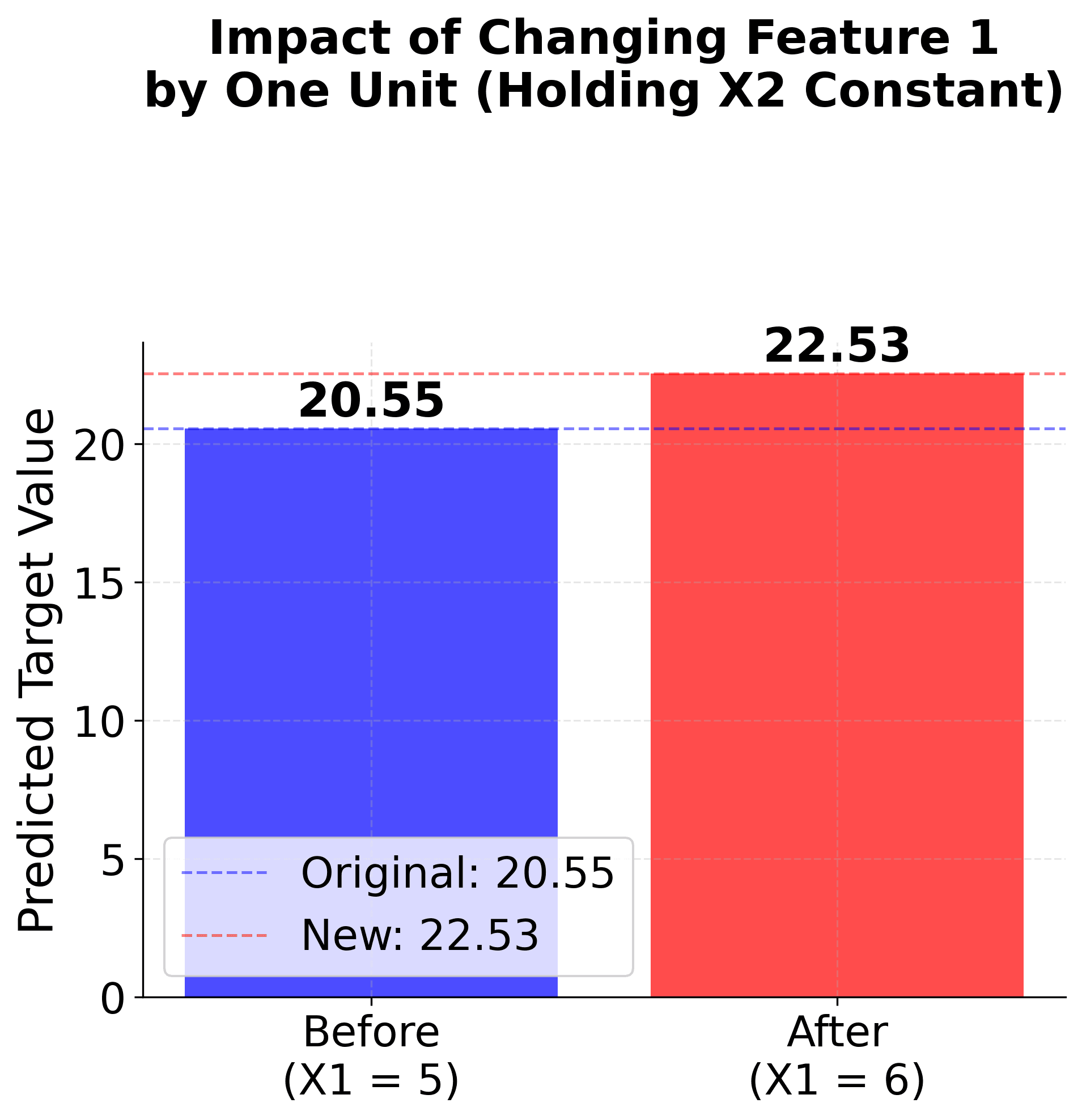
These visualizations make coefficient interpretation concrete and intuitive. The first plot shows the partial effect of one feature while holding others constant, demonstrating that coefficients represent slopes in the relationship between features and target. The second plot shows the practical impact of changing a feature value, making it clear that coefficients represent the expected change in the target variable.
Example
Let's work through a concrete example to see how multiple linear regression works step by step. We'll use a small dataset with two features to make the calculations manageable, and then verify our results using computational tools.
The Dataset
Suppose you're analyzing house prices and have collected data on three houses with two features: size (in square feet) and age (in years). Your target variable is price (in thousands of dollars).
Here's your data:
| House | Size (x₁) | Age (x₂) | Price (y) |
|---|---|---|---|
| 1 | 2,000 | 1 | 6 |
| 2 | 0 | 3 | 10 |
| 3 | 4,000 | 5 | 16 |
Setting Up the Matrices
First, let's organize this data into matrix form. The feature matrix includes a column of ones for the intercept:
Notice that the first column of is all ones—this is crucial for estimating the intercept term .
Step-by-Step OLS Calculation
Now let's compute the OLS solution:
Step 1: Compute
First, we transpose :
Now multiply by :
Let's compute each element:
- :
- :
- :
- :
- :
- :
- :
- :
- :
So:
Step 2: Compute
Computing each element:
- First row:
- Second row:
- Third row:
So:
Step 3: Compute
This is the most complex step. For a 3×3 matrix, we need to compute the determinant and the adjugate matrix. Given the large numbers involved, let's use a computational approach for accuracy.
Step 4: Final Calculation
Using computational tools (which we'll verify in the implementation section), the final result is:
Interpreting the Results
The fitted model is:
where:
-: predicted house price (in thousands of dollars)
- : house size in square feet
- : house age in years
This means:
- Intercept (): A house with zero size and zero age would cost $3{,}000 (though this interpretation doesn't make practical sense)
- Size coefficient (): For each additional square foot, the price increases by $0.33 (0.000333 × 1000)
- Age coefficient (): For each additional year of age, the price increases by $2{,}333
Verification
Let's check how well this model fits our data by calculating predictions for each house:
House 1 (Size = 2000, Age = 1): Actual: → Perfect prediction!
House 2 (Size = 0, Age = 3): Actual: → Perfect prediction!
House 3 (Size = 4000, Age = 5): Actual: → Perfect prediction!
The model provides perfect predictions for this dataset. This is expected because we have exactly as many parameters (3) as data points (3), which allows the model to fit the data exactly. In practice with larger datasets, you would typically see some prediction errors due to noise and the inherent complexity of real-world relationships.
As you can see, even with just three data points and two features, the matrix calculations become quite involved, especially the matrix inversion step. The large numbers (like 20{,}000{,}000) make hand calculations error-prone. This is why we always use computational tools in practice—they're faster, more accurate, and less prone to errors.
Implementation
This section provides a step-by-step tutorial for implementing multiple linear regression using both Scikit-learn and NumPy. We'll start with a simple example to demonstrate the core concepts, then progress to a more realistic scenario that shows how to apply the method in practice.
Step 1: Basic Implementation with Scikit-learn
Let's begin by setting up our data and fitting a multiple linear regression model. We'll use the house price dataset from our mathematical example to demonstrate the core concepts.
Now let's examine the fitted coefficients to understand what the model learned:
The coefficients match our manual calculations exactly! The intercept of 3.0 represents the base price when both size and age are zero. The size coefficient of 0.000333 indicates that each additional square foot increases price by 2{,}333. This demonstrates how multiple linear regression captures the combined effect of multiple features on the target variable.
Step 2: Making Predictions and Evaluating Performance
Let's use the fitted model to make predictions and evaluate its performance:
Perfect predictions with zero error! The of 1.0 indicates that the model explains 100% of the variance in the data. This is expected because we have exactly as many parameters (3) as data points (3), allowing the model to fit the data exactly. In practice with larger datasets, you would typically see some prediction errors due to noise and the inherent complexity of real-world relationships.
Step 3: Understanding the Mathematics with NumPy
For educational purposes, let's implement the multiple linear regression solution from scratch using NumPy to understand the underlying mathematics:
The NumPy implementation produces identical results to Scikit-learn, confirming that both methods use the same mathematical foundation. The np.linalg.solve() function is more numerically stable than computing the matrix inverse explicitly, making it the preferred approach for the multiple linear regression solution.
Step 4: Real-World Example with Larger Dataset
Let's demonstrate multiple linear regression with a more realistic dataset to show how it performs with real-world data:
This example shows how multiple linear regression performs with a more realistic dataset. The model achieves good performance on both training and test sets, with values around 0.95, indicating that the linear model explains most of the variance in the data. The small difference between training and test performance suggests the model generalizes well without overfitting.
Step 5: Model Interpretation and Validation
Let's create a visualization to better understand how our model performs:
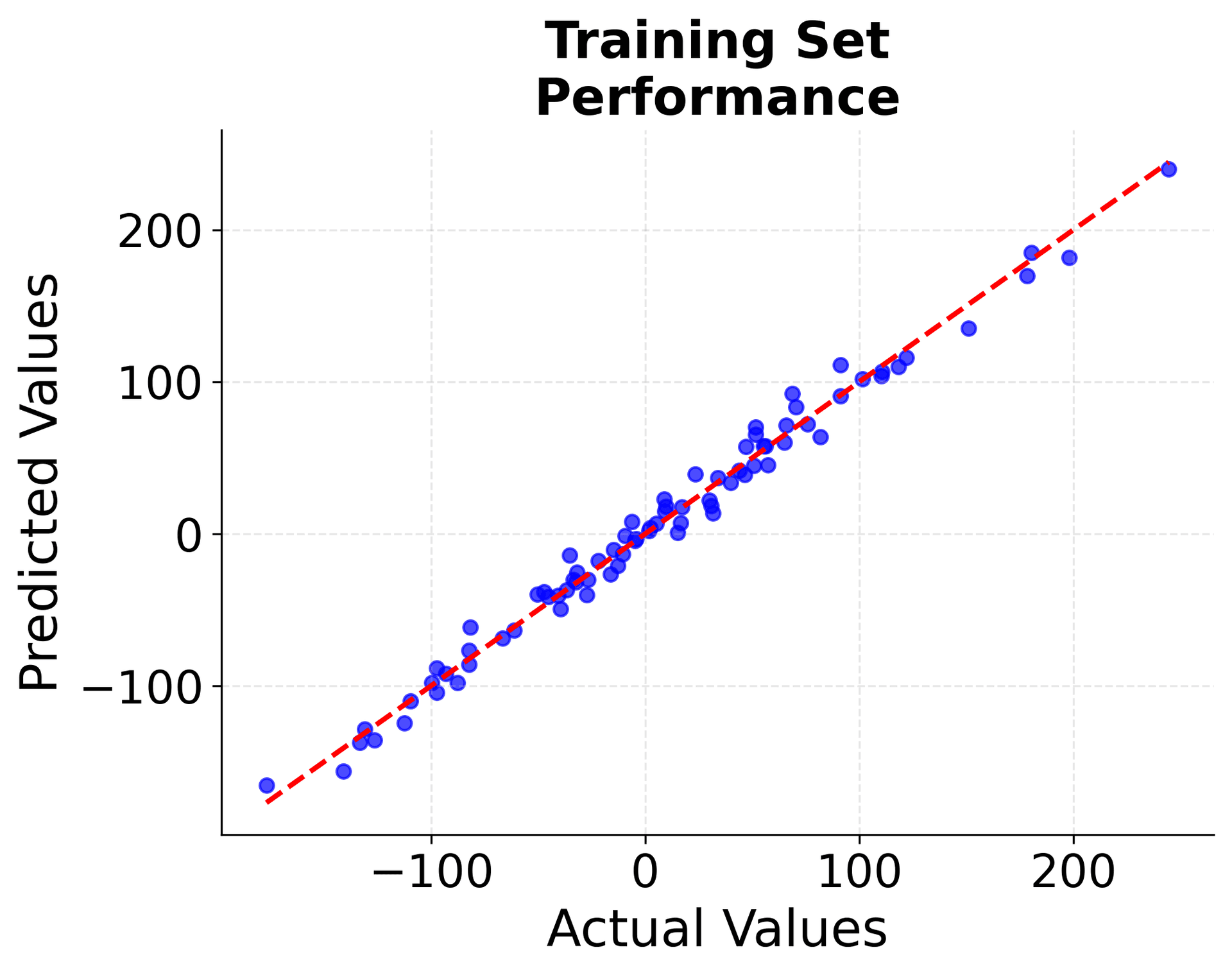
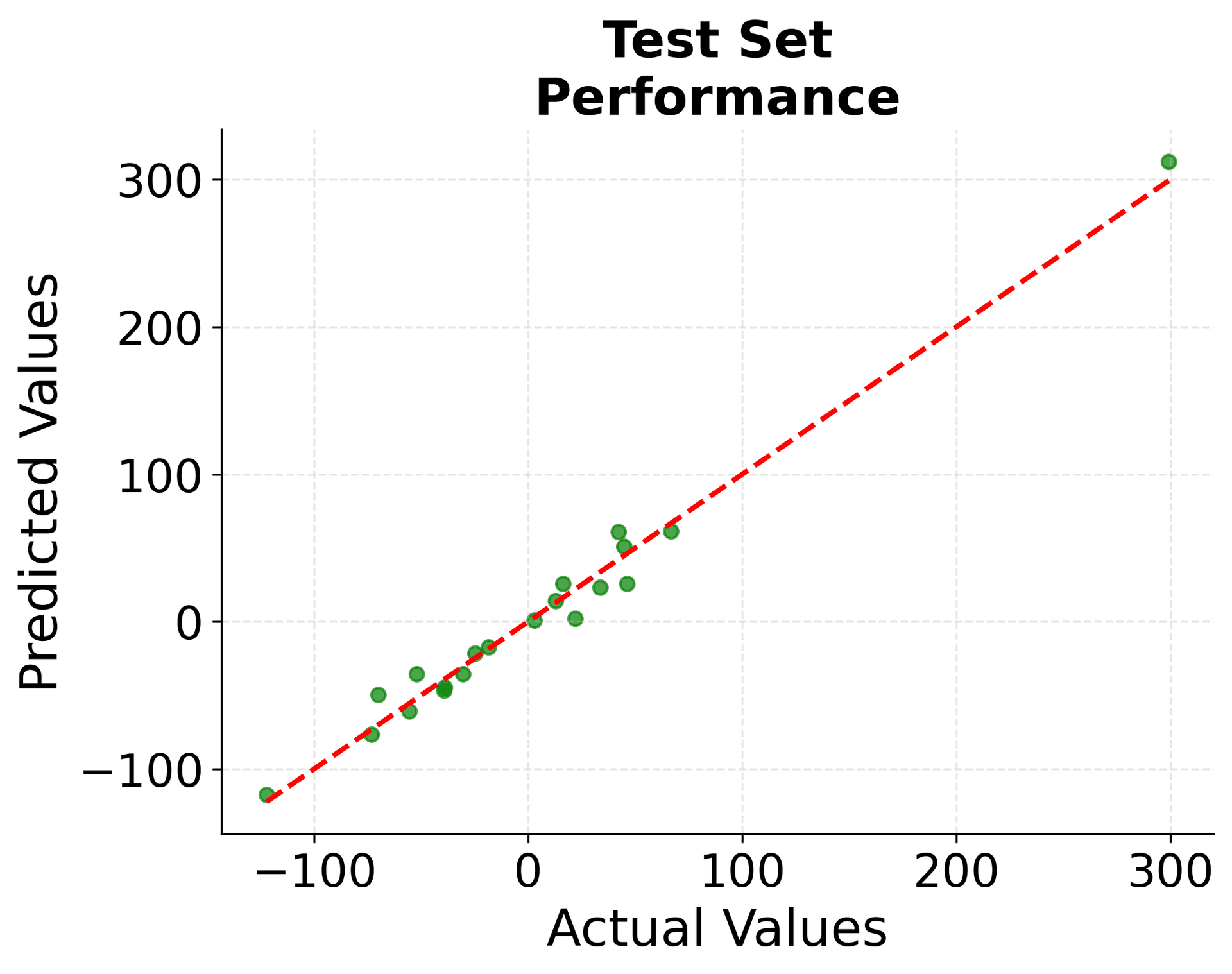
The scatter plots show how well our model predicts the target values. Points close to the red diagonal line indicate accurate predictions. The similar performance on both training and test sets suggests our model generalizes well and doesn't suffer from overfitting.
Key Parameters
Below are the main parameters that affect how the multiple linear regression model works and performs.
fit_intercept: Whether to calculate the intercept for this model. If set to False, no intercept will be used in calculations (i.e., data is expected to be centered). Default: Truecopy_X: If True, X will be copied; else, it may be overwritten. Default: Truen_jobs: The number of jobs to use for the computation. This will only provide speedup for n_targets > 1 and sufficient large problems. Default: None (uses 1 processor)
Key Methods
The following are the most commonly used methods for interacting with the LinearRegression model.
fit(X, y): Fit linear model to training data X and target values y. Returns self for method chainingpredict(X): Predict target values for new data X using the fitted modelscore(X, y): Return the coefficient of determination of the prediction. Best possible score is 1.0get_params(): Get parameters for this estimator. Useful for hyperparameter tuningset_params(**params): Set the parameters of this estimator. Allows parameter modification after initialization
Model Diagnostics: Residual Analysis
After fitting a multiple linear regression model, it's crucial to examine the residuals to validate the model assumptions and identify potential problems. These diagnostic plots help ensure your model is appropriate and reliable.
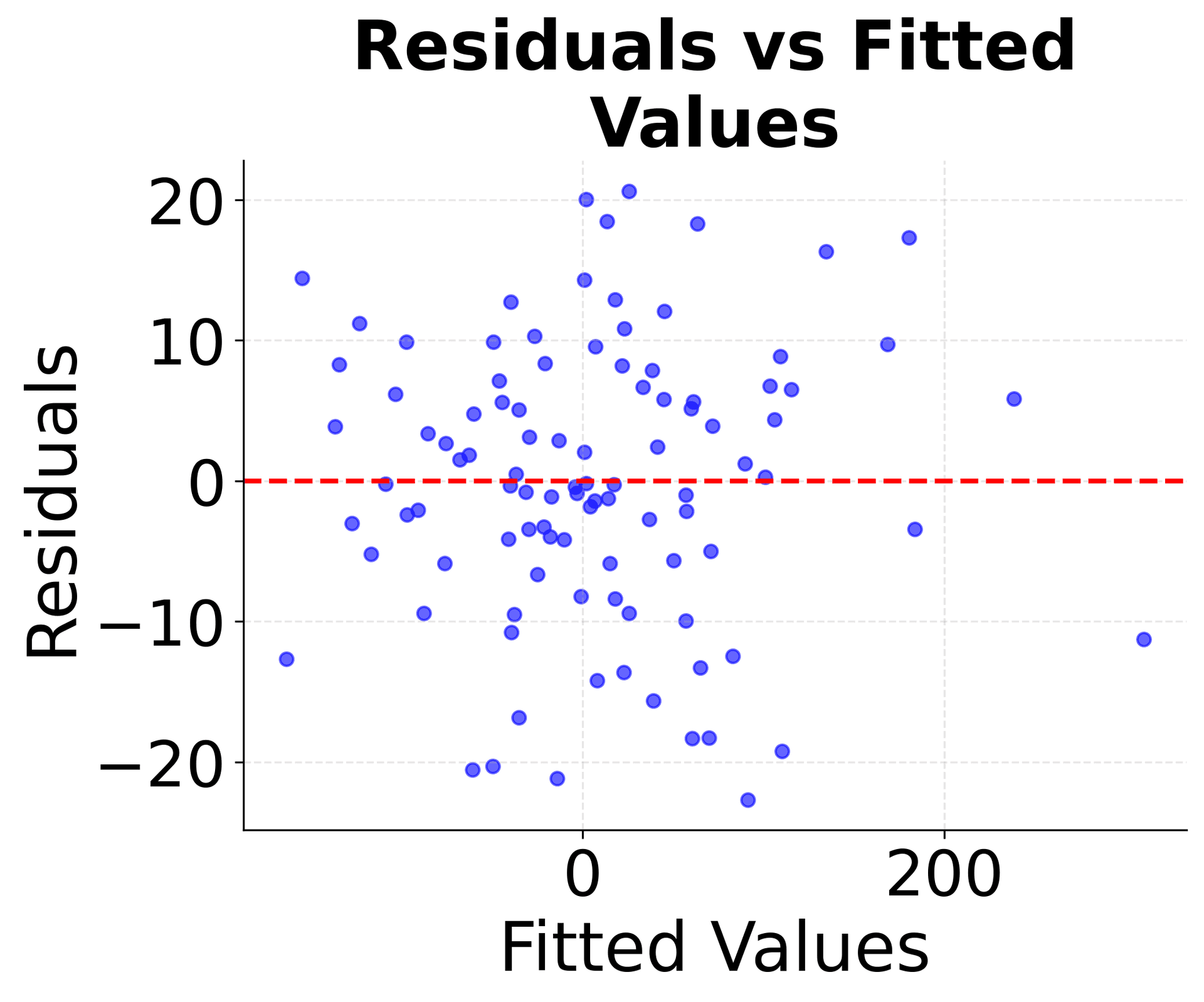
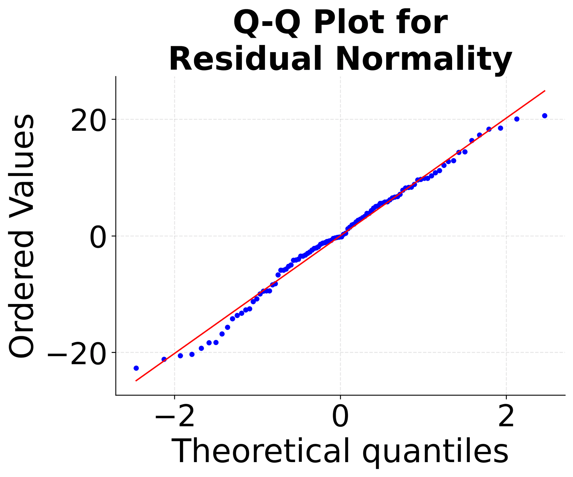
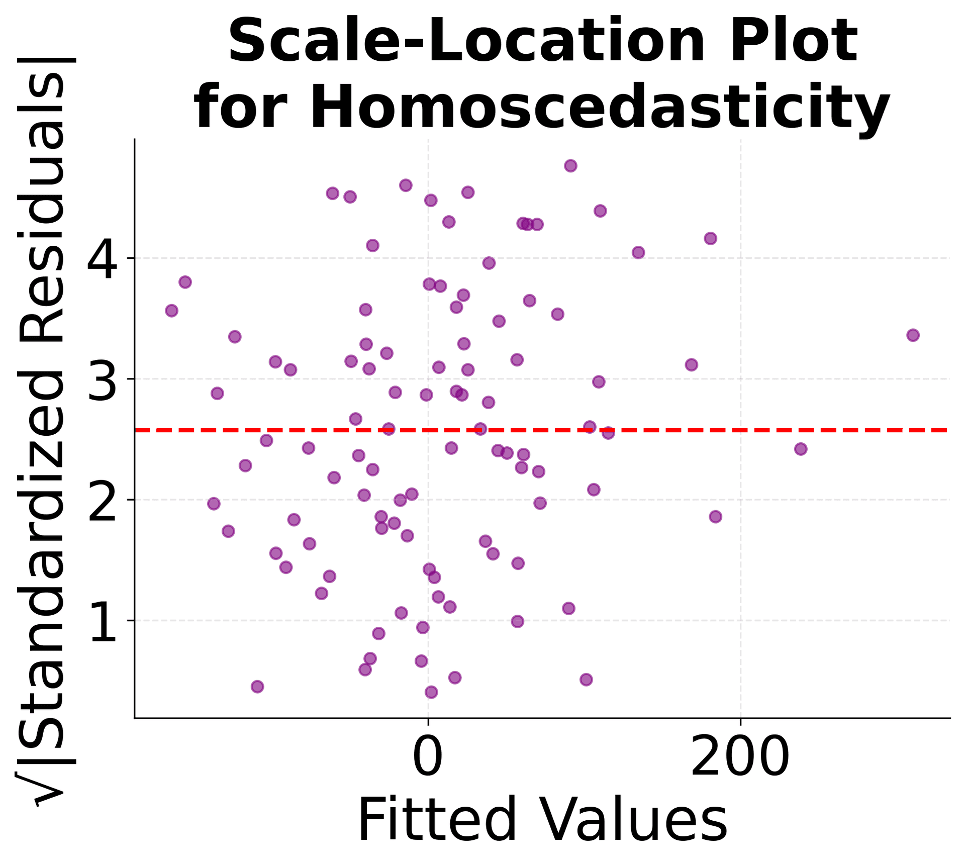
These diagnostic plots are essential for validating your multiple linear regression model. The residuals vs fitted plot checks for linearity and constant variance, the Q-Q plot assesses normality, and the scale-location plot examines homoscedasticity. Together, they help ensure your model meets the necessary assumptions for reliable statistical inference.
Practical Applications
Multiple linear regression is particularly valuable in scenarios where interpretability and statistical inference are important. In business intelligence and decision-making contexts, multiple linear regression excels because it provides clear, actionable insights through coefficient interpretation. Stakeholders can easily understand how each feature affects the outcome, making it ideal for scenarios where model transparency is crucial for regulatory compliance or business justification.
The method is highly effective in exploratory data analysis, where the goal is to understand relationships between variables and identify the most important predictors. Since multiple linear regression provides statistical significance tests for each coefficient, it offers a natural framework for feature selection and hypothesis testing. This makes it particularly useful in scientific research, policy analysis, and any domain where understanding causal relationships is important.
In predictive modeling applications, multiple linear regression serves as an excellent baseline model due to its simplicity and interpretability. When dealing with continuous target variables and linear relationships, it often provides competitive performance while remaining computationally efficient and easy to implement. The method is particularly valuable in domains like real estate pricing, sales forecasting, and risk assessment where linear relationships are common and interpretability is essential.
Best Practices
To achieve optimal results with multiple linear regression, it is important to follow several best practices that address data preparation, model validation, and interpretation. First, always examine your data for linear relationships before applying the model, as the method assumes linearity between features and the target variable. Use scatter plots and correlation analysis to identify potential non-linear patterns that might require transformation or alternative modeling approaches.
When working with multiple features, pay careful attention to multicollinearity, which can make coefficient estimates unstable and difficult to interpret. Calculate variance inflation factors (VIF) for each feature, with values above 5-10 indicating potential multicollinearity problems. Consider removing highly correlated features or using regularization techniques like ridge regression when multicollinearity is present.
For model validation, never rely solely on training set performance metrics. Always use cross-validation or hold-out test sets to assess generalization performance. The difference between training and test performance can reveal overfitting, especially when you have many features relative to your sample size. Aim for consistent performance across different data splits to ensure your model generalizes well.
When interpreting results, combine statistical significance with practical significance. A coefficient might be statistically significant but have negligible practical impact due to the scale of the feature or target variable. Always consider the units of measurement and the business context when evaluating coefficient magnitudes. Use confidence intervals to assess the uncertainty in your estimates and avoid overinterpreting coefficients that have wide confidence intervals.
Finally, always perform comprehensive residual analysis to validate model assumptions. Create diagnostic plots to check for linearity, normality, homoscedasticity, and independence of residuals. These assumptions are crucial for reliable statistical inference and prediction. If assumptions are violated, consider data transformations, alternative modeling approaches, or robust estimation methods to address the issues.
Data Requirements and Pre-processing
Multiple linear regression requires continuous target variables and works best with continuous or properly encoded categorical features. The method assumes linear relationships between features and the target, so data should be examined for non-linear patterns before modeling. Missing values must be handled through imputation or removal, as the algorithm cannot process incomplete observations directly. Outliers can significantly impact coefficient estimates, so robust outlier detection and treatment strategies are essential.
Feature scaling becomes important when coefficients need to be comparable or when using regularization methods. While the algorithm itself doesn't require scaling, standardized features lead to more interpretable coefficients and better numerical stability. Categorical variables must be properly encoded using one-hot encoding for nominal variables or label encoding for ordinal variables with meaningful order. High-cardinality categorical variables may require target encoding or dimensionality reduction techniques.
The method assumes independence of observations, so temporal or spatial autocorrelation can violate this assumption. For time series data, consider using specialized methods or ensuring observations are truly independent. The algorithm also assumes homoscedasticity (constant variance of residuals), so heteroscedastic data may require transformation or alternative modeling approaches.
Common Pitfalls
Some common pitfalls can undermine the effectiveness of multiple linear regression if not carefully addressed. One frequent mistake is ignoring the linearity assumption and applying the method to clearly non-linear relationships, which leads to poor predictions and misleading coefficient interpretations. Another issue arises when multicollinearity is present but not detected, causing coefficient estimates to be unstable and difficult to interpret meaningfully.
Selecting features based solely on statistical significance without considering practical significance can also be problematic, as statistically significant coefficients may have negligible practical impact. It is important to combine statistical tests with effect size measures and domain knowledge to make informed decisions. Ignoring residual analysis can obscure violations of model assumptions, leading to unreliable predictions and incorrect statistical inferences.
Finally, failing to validate model assumptions using diagnostic plots can result in overconfident predictions and misleading conclusions. To ensure robust and meaningful results, always check linearity assumptions, test for multicollinearity, examine residuals thoroughly, consider practical significance alongside statistical significance, and validate all model assumptions before drawing conclusions.
Computational Considerations
Multiple linear regression has computational complexity for the OLS solution, where is the number of observations and is the number of features. For most practical applications, this makes it extremely fast and memory-efficient. However, for very large datasets (typically observations) or high-dimensional data (), memory requirements can become substantial due to the need to store and invert the matrix.
For large datasets, consider using incremental learning algorithms or stochastic gradient descent implementations that can process data in batches. When dealing with high-dimensional data where approaches or exceeds , the OLS solution becomes unstable, and regularization methods like ridge regression become necessary. The algorithm's memory requirements scale quadratically with the number of features, so dimensionality reduction techniques may be required for very high-dimensional problems.
Performance and Deployment Considerations
Multiple linear regression performance is typically evaluated using , adjusted , mean squared error (MSE), and root mean squared error (RMSE). Good performance indicators include values above 0.7 for most applications, though this varies by domain. Cross-validation scores should be close to training scores to indicate good generalization. Residual analysis should show random scatter around zero without systematic patterns.
For deployment, the model's simplicity makes it highly scalable and suitable for real-time prediction systems. The linear nature of predictions allows for efficient computation even with large feature sets. However, the model's performance can degrade significantly if the underlying relationships change over time, so regular retraining may be necessary. The interpretable nature of coefficients makes it easy to monitor model behavior and detect when retraining is needed.
In production environments, multiple linear regression models are typically deployed as simple mathematical functions, making them easy to implement across different platforms and programming languages. The model's transparency also facilitates regulatory compliance and makes it easier to explain predictions to stakeholders. However, the linear assumption means the model may not capture complex non-linear relationships that could be important for optimal performance.
Summary
Multiple linear regression is a fundamental and powerful technique that extends simple linear regression to handle multiple features simultaneously. By fitting a hyperplane through data points, it finds the optimal combination of feature weights that best predicts the target variable.
The method's strength lies in its mathematical elegance and interpretability. The OLS solution provides a closed-form solution that's both computationally efficient and statistically optimal under standard assumptions. Each coefficient tells you exactly how much the target variable changes when you increase the corresponding feature by one unit, holding all other features constant.
While the linearity assumption may seem restrictive, multiple linear regression often performs well in practice and serves as an excellent baseline for more complex models. Its interpretability makes it invaluable for business applications where understanding the relationship between features and outcomes is as important as making accurate predictions.
The key to success with multiple linear regression lies in proper data preprocessing, thoughtful feature selection, and careful validation. When applied correctly, it provides a solid foundation for understanding data and building reliable predictive models that stakeholders can trust and act upon.
Quiz
Ready to test your understanding of multiple linear regression? Take this quiz to reinforce what you've learned about modeling relationships with multiple predictors.


Comments