InteractiveHierarchical Clustering: Complete Guide with Dendrograms, Linkage Criteria & Implementation

Hierarchical Clustering

Hierarchical clustering is a powerful unsupervised learning technique that builds a hierarchy of clusters by either merging smaller clusters into larger ones (agglomerative) or splitting larger clusters into smaller ones (divisive). Unlike k-means clustering, which requires us to specify the number of clusters beforehand, hierarchical clustering creates a complete hierarchy that allows us to examine clusters at different levels of granularity.

The key insight behind hierarchical clustering is that data points can be organized into a tree-like structure called a dendrogram, where the height of branches represents the distance between clusters. This dendrogram provides a complete picture of how data points relate to each other at different scales, making it particularly valuable for exploratory data analysis and when we're uncertain about the optimal number of clusters.

Hierarchical clustering differs from other clustering methods in several important ways. While k-means assumes spherical clusters and requires us to specify k in advance, hierarchical clustering makes no assumptions about cluster shape and provides a complete clustering solution for all possible numbers of clusters. Unlike density-based methods like DBSCAN, hierarchical clustering doesn't require tuning parameters like minimum points or epsilon radius, though it does require choosing a distance metric and linkage criterion.

The method is particularly well-suited for datasets where we expect natural hierarchical relationships, such as biological taxonomy, organizational structures, or any domain where objects naturally group into nested categories. The dendrogram visualization makes it easy to understand the clustering structure and identify natural cut points for different numbers of clusters.

Advantages

Hierarchical clustering offers several compelling advantages that make it a valuable tool in the data scientist's toolkit. First, it provides a complete clustering solution for all possible numbers of clusters in a single run, eliminating the need to run the algorithm multiple times with different k values. This is particularly advantageous when we're uncertain about the optimal number of clusters or when we want to explore the data at multiple levels of granularity.

The dendrogram visualization is another major strength, providing an intuitive way to understand the clustering structure and relationships between data points. This visual representation makes it easy to identify natural cluster boundaries and understand how clusters merge or split as we move up or down the hierarchy. The dendrogram also helps in determining the optimal number of clusters by identifying significant gaps in the merging distances.

Unlike k-means, hierarchical clustering doesn't require us to specify the number of clusters in advance, making it well-suited for exploratory data analysis. It also doesn't assume spherical clusters, allowing it to capture more complex cluster shapes. The deterministic nature of the algorithm means that given the same data and parameters, it typically produces the same results, which is valuable for reproducible research.

Disadvantages

Despite its strengths, hierarchical clustering has several limitations that can impact its practical application. The most significant drawback is its computational complexity, which is O(n³) for most implementations. This makes it computationally expensive for large datasets, often limiting its use to datasets with fewer than several thousand points. For very large datasets, the memory requirements can also become prohibitive.

The algorithm is sensitive to noise and outliers, which can significantly affect the clustering results. A single outlier can create spurious clusters or distort the entire hierarchy, making the dendrogram less interpretable. This sensitivity means that data preprocessing and outlier detection become crucial steps before applying hierarchical clustering.

Another limitation is that hierarchical clustering doesn't perform well with clusters of very different sizes or densities. The algorithm tends to favor clusters of similar sizes, which can lead to poor results when the true clusters have dramatically different characteristics. Additionally, once a data point is assigned to a cluster, it cannot be reassigned, which can lead to suboptimal clustering if early decisions were made based on limited information.

The choice of distance metric and linkage criterion can significantly affect the results, and there's often no clear guidance on which combination works best for a particular dataset. This parameter sensitivity means that extensive experimentation may be required to find the optimal configuration, adding to the computational burden.

Formula

Imagine you're organizing a library. You start with individual books scattered on tables, and your goal is to arrange them into meaningful groups, perhaps by genre, then by author, then by publication date. As you work, you notice that some books naturally belong together, while others form distinct groups. This intuitive process of building organization from the bottom up, creating nested categories that reflect natural relationships, is exactly what hierarchical clustering does with data.

The mathematical challenge is significant: given a collection of data points, how do we discover and represent their natural hierarchical relationships? Unlike methods that require us to specify the number of groups in advance, hierarchical clustering builds a complete tree of relationships, called a dendrogram, that reveals how data points connect at every possible level of granularity. This tree shows us which points belong together, how they relate, when they merge, and why certain groupings make sense.

To build this hierarchy, we need to solve three fundamental problems in sequence:

1. Measuring similarity between individual points: How do we quantify how similar or different any two data points are?
2. Measuring similarity between groups of points: Once we have clusters, how do we decide which clusters should merge next?
3. Building the hierarchy systematically: How do we combine these measurements into an algorithm that creates a meaningful tree structure?

Each problem builds naturally on the previous one, and together they form a complete mathematical framework for hierarchical clustering. Let's explore each piece, understanding not just what the formulas say, but why they're necessary and how they work together to solve the clustering problem.

The Foundation: Measuring Distance Between Points

Before we can group points into clusters, we need a fundamental tool: a way to measure how similar or different any two points are. This might seem straightforward, but the choice of measurement profoundly affects what clusters we discover. Think of it like choosing between measuring distance "as the crow flies" versus "along city streets." The same two locations can appear very different depending on your metric.

In data science, we work with points that have multiple features. A customer might be described by age, income, and purchase frequency. A gene might be characterized by expression levels across hundreds of conditions. A document might be represented by word frequencies across thousands of terms. To measure similarity, we need a way to combine differences across all these dimensions into a single number.

The Euclidean Distance: Our Intuitive Starting Point

The most natural approach is to measure the straight-line distance between points, just as we would measure the distance between two cities on a map. This is the Euclidean distance, and it captures our intuitive sense of "closeness" in multidimensional space.

For two data points $\mathbf{x}_i$ and $\mathbf{x}_j$ in a d-dimensional space, the Euclidean distance is:

where:

• $\mathbf{x}_i$: the $i$-th data point (a vector with $d$ features)
• $\mathbf{x}_j$: the $j$-th data point (a vector with $d$ features)
• $d$: the number of features (dimensions) in the data space
• $x_{ik}$: the value of the $k$-th feature for the $i$-th data point
• $x_{jk}$: the value of the $k$-th feature for the $j$-th data point
• $k$: index over features, ranging from 1 to $d$

Let's understand what each part of this formula accomplishes:

• $(x_{ik} - x_{jk})$: For each feature $k$, we compute how different the two points are. This difference can be positive or negative, depending on which point has the larger value.
• $(x_{ik} - x_{jk})^2$: We square each difference. This serves two crucial purposes: it ensures all terms are positive (so differences in opposite directions don't cancel out), and it gives more weight to larger differences. A difference of 10 contributes 100 to the sum, while a difference of 1 contributes only 1.
• $\sum_{k=1}^{d}$: We sum these squared differences across all $d$ features, combining differences in age, income, purchase frequency, and every other dimension into a single measure.
• $\sqrt{\cdot}$: Finally, we take the square root to return to the original units of measurement. Without this, we'd be working with squared distances, which would be harder to interpret and wouldn't have the same units as our original features.

The square root is more than a mathematical convenience. It ensures that if point A is twice as far from point B as point C is from point D, our distance metric reflects this relationship proportionally.

The Scale Problem: Why Standardization Matters

However, there's an important problem that emerges in real-world data: features often have dramatically different scales. Consider clustering customers using age (ranging from 18 to 80 years) and annual income (ranging from $20,000 to $200,000). In the Euclidean distance calculation, a $10,000 difference in income contributes $(10,000)^2 = 100,000,000$ to the squared distance sum, while a 10-year difference in age contributes only $10^2 = 100$. Income largely dominates the distance calculation, making age largely irrelevant to the clustering.

This isn't just a mathematical curiosity. It means our clusters will be determined almost entirely by income, ignoring potentially important patterns related to age. We need a way to ensure that all features contribute meaningfully to the distance calculation, regardless of their original scales.

The Solution: Standardized Euclidean Distance

The solution is to normalize each feature by its variability before computing distances. This gives us the standardized Euclidean distance:

where:

• $\mathbf{x}_i$: the $i$-th data point (a vector with $d$ features)
• $\mathbf{x}_j$: the $j$-th data point (a vector with $d$ features)
• $d$: the number of features (dimensions) in the data space
• $x_{ik}$: the value of the $k$-th feature for the $i$-th data point
• $x_{jk}$: the value of the $k$-th feature for the $j$-th data point
• $s_k$: the standard deviation of the $k$-th feature across all data points
• $k$: index over features, ranging from 1 to $d$

By dividing each squared difference by $s_k^2$, we're essentially asking: "How many standard deviations apart are these two points on this feature?" This normalization ensures that:

• A one-standard-deviation difference in age contributes the same amount to the distance as a one-standard-deviation difference in income
• Features with larger scales don't dominate the calculation
• All features contribute meaningfully to determining which points are similar

This is why standardization is typically an important preprocessing step before hierarchical clustering. Without it, we're not discovering the true structure of our data. We're just finding patterns in whichever feature happens to have the largest numbers.

The Bridge: Measuring Distance Between Clusters

Once we can measure distances between individual points, we face a new and more subtle challenge: how do we measure the distance between two clusters, each of which may contain multiple points? This question is fundamental because hierarchical clustering repeatedly merges clusters, and at each step, we need a rule to decide which clusters are most similar and should merge next.

The challenge is that a cluster isn't a single point. It's a collection of points that may be spread out in various ways. Two clusters might each contain 100 points arranged in different patterns: one might be a tight, compact sphere, while another might be an elongated ellipse. How do we capture the "distance" between such complex objects?

This is where linkage criteria come into play. A linkage criterion defines how we compute the distance between two clusters based on the distances between the individual points within them. The choice of linkage criterion is one of the most important decisions in hierarchical clustering because it fundamentally shapes what kinds of clusters we discover.

Different linkage criteria answer different questions about cluster similarity, and each leads to distinct clustering behaviors. Understanding these criteria isn't just about memorizing formulas. It's about understanding what question each one asks and what kind of answer it provides.

Single Linkage: The Optimistic Criterion

The simplest approach is to define the distance between two clusters as the distance between their two closest points. This is called single linkage (also known as minimum linkage):

where:

• $A$: the first cluster (a set of data points)
• $B$: the second cluster (a set of data points)
• $a$: a data point belonging to cluster $A$
• $b$: a data point belonging to cluster $B$
• $d(a, b)$: the distance between points $a$ and $b$ (using the chosen distance metric)
• $\min$: the minimum operator (finds the smallest value)

Think of this as asking: "What's the shortest bridge between these two clusters?" If even one point from cluster A is close to one point from cluster B, the clusters are considered similar and likely to merge.

This lenient criterion has important consequences:

• It creates elongated, chain-like clusters: Because only one pair of points needs to be close, clusters can connect through narrow "bridges" of points. This is called the "chaining effect." Imagine a chain where each link is close to the next, even though the endpoints are far apart.
• It's sensitive to outliers: A single outlier point can create a spurious connection between otherwise distant clusters, distorting the entire hierarchy.
• It captures non-spherical clusters: Unlike methods that assume clusters are round, single linkage can discover clusters of arbitrary shape, as long as they're connected by a path of nearby points.

Single linkage is like an optimistic friend who sees connections everywhere. It's great for finding complex, non-linear structures, but it can also create clusters that don't reflect meaningful groupings.

Complete Linkage: The Pessimistic Criterion

At the opposite extreme, complete linkage (also known as maximum linkage) defines the distance between two clusters as the distance between their two farthest points:

where:

• $A$: the first cluster (a set of data points)
• $B$: the second cluster (a set of data points)
• $a$: a data point belonging to cluster $A$
• $b$: a data point belonging to cluster $B$
• $d(a, b)$: the distance between points $a$ and $b$ (using the chosen distance metric)
• $\max$: the maximum operator (finds the largest value)

This is like asking: "What's the longest gap we'd need to bridge to connect these clusters?" This strict criterion requires that all points in the resulting merged cluster be relatively close to each other.

Complete linkage has very different characteristics:

• It creates compact, spherical clusters: Because it considers the worst-case distance, complete linkage tends to produce tight, ball-shaped clusters where all points are close together.
• It's less sensitive to outliers: A single outlier won't dramatically affect the cluster distance, since we're looking at the maximum distance anyway.
• It may break up natural clusters: If a natural cluster isn't perfectly spherical, perhaps it's elongated or has a complex shape, complete linkage may split it into multiple smaller clusters.

Complete linkage is like a perfectionist who wants everything to be tightly organized. It creates clean, compact groups, but it might miss clusters that don't fit the "round" assumption.

Average Linkage: The Balanced Approach

Between these two extremes, average linkage provides a balanced approach by considering all pairwise distances between points in the two clusters:

where:

• $A$: the first cluster (a set of data points)
• $B$: the second cluster (a set of data points)
• $|A|$: the number of data points in cluster $A$ (cardinality of set $A$)
• $|B|$: the number of data points in cluster $B$ (cardinality of set $B$)
• $a$: a data point belonging to cluster $A$
• $b$: a data point belonging to cluster $B$
• $d(a, b)$: the distance between points $a$ and $b$ (using the chosen distance metric)
• $\sum$: the summation operator (sums over all pairs of points)

This formula computes the average of all possible distances between points in cluster A and points in cluster B. By considering every pair, average linkage provides a comprehensive measure of cluster similarity that:

• Balances compactness and flexibility: It's stricter than single linkage (requiring overall similarity, not just one close pair) but more flexible than complete linkage (not requiring the worst-case distance to be small).
• Reflects the overall relationship: Rather than focusing on the best or worst connection, it considers the typical relationship between clusters.
• Often matches real-world structure: In practice, average linkage tends to produce clusters that better reflect the natural structure of real-world data, making it a popular default choice.

Average linkage is like a thoughtful analyst who considers all the evidence. It provides a balanced view that often captures meaningful patterns without the extremes of optimism or perfectionism.

The choice of linkage criterion fundamentally shapes what clusters we discover. Single linkage finds chains and complex shapes but can create spurious connections. Complete linkage finds compact spheres but may miss natural elongated clusters. Average linkage provides a practical middle ground that often works well in practice. Understanding these trade-offs helps us choose the right criterion for our specific data and goals.

Building the Hierarchy: The Agglomerative Algorithm

Now that we understand how to measure distances between points and between clusters, we can assemble these pieces into a complete algorithm. The word "agglomerative" means "to collect into a mass," which describes what this algorithm does: it starts with individual points and gradually collects them into larger and larger clusters, building a complete hierarchy in the process.

The algorithm's strategy is straightforward: begin with each data point as its own cluster, then repeatedly merge the two most similar clusters until everything belongs to one big cluster. This process creates a complete hierarchy of clusterings, from $n$ clusters (one per point) all the way down to 1 cluster (everything together). A key property of this approach is that we get a solution for every possible number of clusters in a single run. We can examine the data at any level of granularity we choose.

Let's walk through the algorithm step by step, understanding not just what each step does, but why it's necessary and how it builds toward the complete hierarchy.

Step 1: Initialize with Individual Points

We start with the simplest possible clustering: each data point is its own cluster. If we have $n$ data points, we have $n$ clusters:

$C_1 = \{x_1\}, C_2 = \{x_2\}, \ldots, C_n = \{x_n\}$

where:

• $n$: the total number of data points in the dataset
• $C_i$: the $i$-th cluster (initially containing only point $x_i$)
• $x_i$: the $i$-th data point (a vector with $d$ features)
• $\{x_i\}$: a set containing only the point $x_i$

At this stage, every cluster contains exactly one point, so there's no ambiguity about cluster membership. This initialization is crucial because it gives us a clean starting point where we know exactly what each cluster contains. From here, we'll build upward, merging clusters to create larger groups.

Step 2: Compute the Initial Distance Matrix

Next, we calculate the distance between every pair of clusters. Initially, since each cluster contains only one point, this is simply the distance between individual points using our chosen distance metric (Euclidean, standardized Euclidean, etc.):

$D_{ij} = d(x_i, x_j) \quad \text{for all } i, j \in \{1, 2, \ldots, n\}$

where:

• $D_{ij}$: the distance between clusters $C_i$ and $C_j$ (entry in row $i$, column $j$ of the distance matrix)
• $d(x_i, x_j)$: the distance between data points $x_i$ and $x_j$ (using the chosen distance metric)
• $x_i$: the $i$-th data point
• $x_j$: the $j$-th data point
• $i, j$: indices ranging from 1 to $n$
• $n$: the total number of data points

This creates an $n \times n$ distance matrix where entry $D_{ij}$ tells us how far apart clusters $C_i$ and $C_j$ are. The matrix has several important properties:

• Symmetry: $D_{ij} = D_{ji}$ (distance from $i$ to $j$ equals distance from $j$ to $i$)
• Zero diagonal: $D_{ii} = 0$ (each point is distance zero from itself)
• Triangle inequality: For most distance metrics, $D_{ik} \leq D_{ij} + D_{jk}$ (the direct distance is never longer than going through an intermediate point)

This distance matrix is our "map" of relationships between all points. It tells us, at a glance, which points are similar and which are different.

Step 3: Find the Closest Clusters

Now we search through our distance matrix to find the pair of clusters that are closest together:

$(i^*, j^*) = \arg\min_{i,j} D_{ij}$

where:

• $i^*$: the index of the first cluster in the closest pair
• $j^*$: the index of the second cluster in the closest pair
• $D_{ij}$: the distance between clusters $C_i$ and $C_j$
• $\arg\min$: the argument of the minimum operator (finds the indices that minimize the distance)
• $i, j$: indices ranging over all pairs of clusters

The notation $\arg\min$ means "find the arguments (indices) that minimize the distance." In other words, we're finding which two clusters have the smallest distance between them. These are the clusters we'll merge next.

This step embodies the core principle of hierarchical clustering: merge the most similar clusters first. This greedy approach, making the locally optimal choice at each step, is what makes the algorithm computationally tractable. While it doesn't guarantee a globally optimal clustering (which would be computationally intractable), it produces meaningful hierarchies that reflect the natural structure of the data.

Step 4: Merge the Closest Clusters

We combine the two closest clusters into a single new cluster:

$C_{new} = C_{i^*} \cup C_{j^*}$

where:

• $C_{new}$: the newly created cluster formed by merging $C_{i^*}$ and $C_{j^*}$
• $C_{i^*}$: the first cluster to be merged (the cluster at index $i^*$)
• $C_{j^*}$: the second cluster to be merged (the cluster at index $j^*$)
• $\cup$: the set union operator (combines all points from both clusters)

The union symbol ($\cup$) means we're taking all points from both clusters and putting them together. After this merge, we now have $n-1$ clusters instead of $n$. This reduction continues with each merge until we eventually have just one cluster containing all points.

Step 5: Update the Distance Matrix

This is where the algorithm gets particularly interesting. After merging two clusters, we need to update our distance matrix to reflect the new cluster structure. We remove the rows and columns corresponding to the two merged clusters and add a new row and column for the merged cluster.

The distance from the new cluster $C_{new}$ to any other cluster $C$ is calculated using our chosen linkage criterion:

$d(C_{new}, C) = \text{linkage\_function}(C_{i^*}, C_{j^*}, C)$

The exact formula depends on which linkage criterion we're using:

• Single linkage: $d(C_{new}, C) = \min(d(C_{i^*}, C), d(C_{j^*}, C))$
• Complete linkage: $d(C_{new}, C) = \max(d(C_{i^*}, C), d(C_{j^*}, C))$
• Average linkage: $d(C_{new}, C) = \frac{|C_{i^*}|}{|C_{new}|} \cdot d(C_{i^*}, C) + \frac{|C_{j^*}|}{|C_{new}|} \cdot d(C_{j^*}, C)$

where:

• $C_{new}$: the newly merged cluster ($C_{i^*} \cup C_{j^*}$)
• $C$: any other existing cluster
• $C_{i^*}$: the first cluster that was merged to form $C_{new}$
• $C_{j^*}$: the second cluster that was merged to form $C_{new}$
• $d(C_{i^*}, C)$: the distance from cluster $C_{i^*}$ to cluster $C$ (from the previous distance matrix)
• $d(C_{j^*}, C)$: the distance from cluster $C_{j^*}$ to cluster $C$ (from the previous distance matrix)
• $|C_{i^*}|$: the number of points in cluster $C_{i^*}$
• $|C_{j^*}|$: the number of points in cluster $C_{j^*}$
• $|C_{new}|$: the number of points in the merged cluster ($|C_{i^*}| + |C_{j^*}|$)

The key insight is that we can compute these distances efficiently using only the existing distances and cluster sizes, without recalculating all pairwise distances from scratch. This efficiency is crucial for making the algorithm practical on real datasets.

Step 6: Repeat Until Complete

We repeat steps 3-5, each time merging the two closest clusters, until only one cluster remains. This process creates a binary tree structure called a dendrogram, where:

• Each leaf node represents an individual data point
• Each internal node represents a merge operation
• The height of each node corresponds to the distance at which the clusters were merged

The dendrogram is more than just a visualization. It's a complete record of the clustering process. By "cutting" the dendrogram at different heights, we can extract different numbers of clusters, making it easy to explore the data at multiple levels of granularity. A large gap in the merging distances (a long horizontal line in the dendrogram) suggests a natural separation point where clusters are clearly distinct.

Understanding the Algorithm's Mathematical Properties

The hierarchical clustering algorithm has several important mathematical properties that shape both its behavior and its limitations. Understanding these properties helps us appreciate why the algorithm works well in some situations and struggles in others.

The Greedy Nature: Local Optimality

Hierarchical clustering is a greedy algorithm, meaning that at each step, it makes the locally optimal choice (merging the two closest clusters) without considering how this decision might affect future merges. Like a chess player who makes the best immediate move without thinking several moves ahead, the algorithm can sometimes make choices that lead to suboptimal overall clustering.

However, this greedy approach is what makes the algorithm computationally tractable. If we tried to find the globally optimal clustering by considering all possible merge sequences, the problem would become computationally intractable for even moderately sized datasets. The number of possible cluster hierarchies grows exponentially with the number of points, making exhaustive search impractical.

The greedy strategy works well in practice because natural clusters tend to be well-separated. If two points belong together, they'll be close at every level of the hierarchy. The algorithm's local decisions usually align with the global structure we want to discover.

The Dendrogram: A Complete Hierarchy

The algorithm produces a binary tree structure called a dendrogram, where each internal node represents a merge operation. The height of each node in the dendrogram corresponds to the distance at which the clusters were merged. This visualization is powerful because it shows the complete clustering hierarchy at a glance.

The dendrogram has several important properties:

• Completeness: It contains information about clustering at every possible number of clusters, from $n$ down to 1
• Monotonicity: The merge distances are non-decreasing as we move up the tree (clusters merge at increasing distances)
• Interpretability: Large gaps in merge distances indicate natural cluster boundaries

By examining the dendrogram, we can identify natural cut points. These are heights where clusters were merged at much larger distances than previous merges, suggesting that the clusters below this point are clearly distinct.

Efficient Distance Updates: The Lance-Williams Formula

The distance matrix update step is crucial for maintaining the algorithm's efficiency. After each merge, we could recalculate all distances from scratch by computing distances between all pairs of points in the new and existing clusters, but this would be computationally expensive.

Instead, we use update formulas that allow us to compute the distance from the newly merged cluster to any other cluster using only the existing distances and cluster sizes. For average linkage, this is the Lance-Williams formula:

$d(C_{new}, C) = \frac{|C_{i^*}|}{|C_{i^*}| + |C_{j^*}|} \cdot d(C_{i^*}, C) + \frac{|C_{j^*}|}{|C_{i^*}| + |C_{j^*}|} \cdot d(C_{j^*}, C)$

where:

• $C_{new}$: the newly merged cluster ($C_{i^*} \cup C_{j^*}$)
• $C$: any other existing cluster
• $C_{i^*}$: the first cluster that was merged to form $C_{new}$
• $C_{j^*}$: the second cluster that was merged to form $C_{new}$
• $d(C_{new}, C)$: the distance from the merged cluster $C_{new}$ to cluster $C$
• $d(C_{i^*}, C)$: the distance from cluster $C_{i^*}$ to cluster $C$ (from the previous distance matrix)
• $d(C_{j^*}, C)$: the distance from cluster $C_{j^*}$ to cluster $C$ (from the previous distance matrix)
• $|C_{i^*}|$: the number of points in cluster $C_{i^*}$
• $|C_{j^*}|$: the number of points in cluster $C_{j^*}$

This formula is a weighted average of the distances from the two original clusters to cluster $C$, where the weights are proportional to the sizes of the original clusters. The larger cluster gets more weight in the calculation, which makes intuitive sense: if cluster $A$ has 100 points and cluster $B$ has 10 points, the merged cluster's distance to $C$ should be closer to $A$'s distance than to $B$'s distance.

This efficient update mechanism is what makes hierarchical clustering practical for datasets with thousands of points, even though the overall complexity is still $O(n^3)$ for computing the initial distance matrix and $O(n^2)$ for the merging process. Without these update formulas, the algorithm would be prohibitively slow for even moderate-sized datasets.

Computational Complexity: The Trade-off

The algorithm's computational requirements are an important consideration:

• Time complexity: $O(n^3)$ for most implementations, due to the need to compute and update the distance matrix
• Space complexity: $O(n^2)$ for storing the distance matrix
• Practical limits: Typically used for datasets with fewer than several thousand points

This complexity is the price we pay for the algorithm's completeness, which is the ability to examine clustering at every possible level of granularity. For larger datasets, we often need to use sampling strategies, approximate methods, or alternative clustering algorithms that scale better.

Together, these mathematical properties (the greedy strategy, the complete dendrogram, and the efficient update mechanisms) define how hierarchical clustering works and when it's most appropriate to use. The algorithm's strength lies in providing a complete, interpretable hierarchy that reveals the natural structure of data at multiple scales, while its limitations come from computational requirements and sensitivity to certain data characteristics.

Visualizing Hierarchical Clustering

Let's create visualizations that demonstrate the key concepts of hierarchical clustering, including how different linkage criteria affect the clustering results and how dendrograms reveal the hierarchical structure.

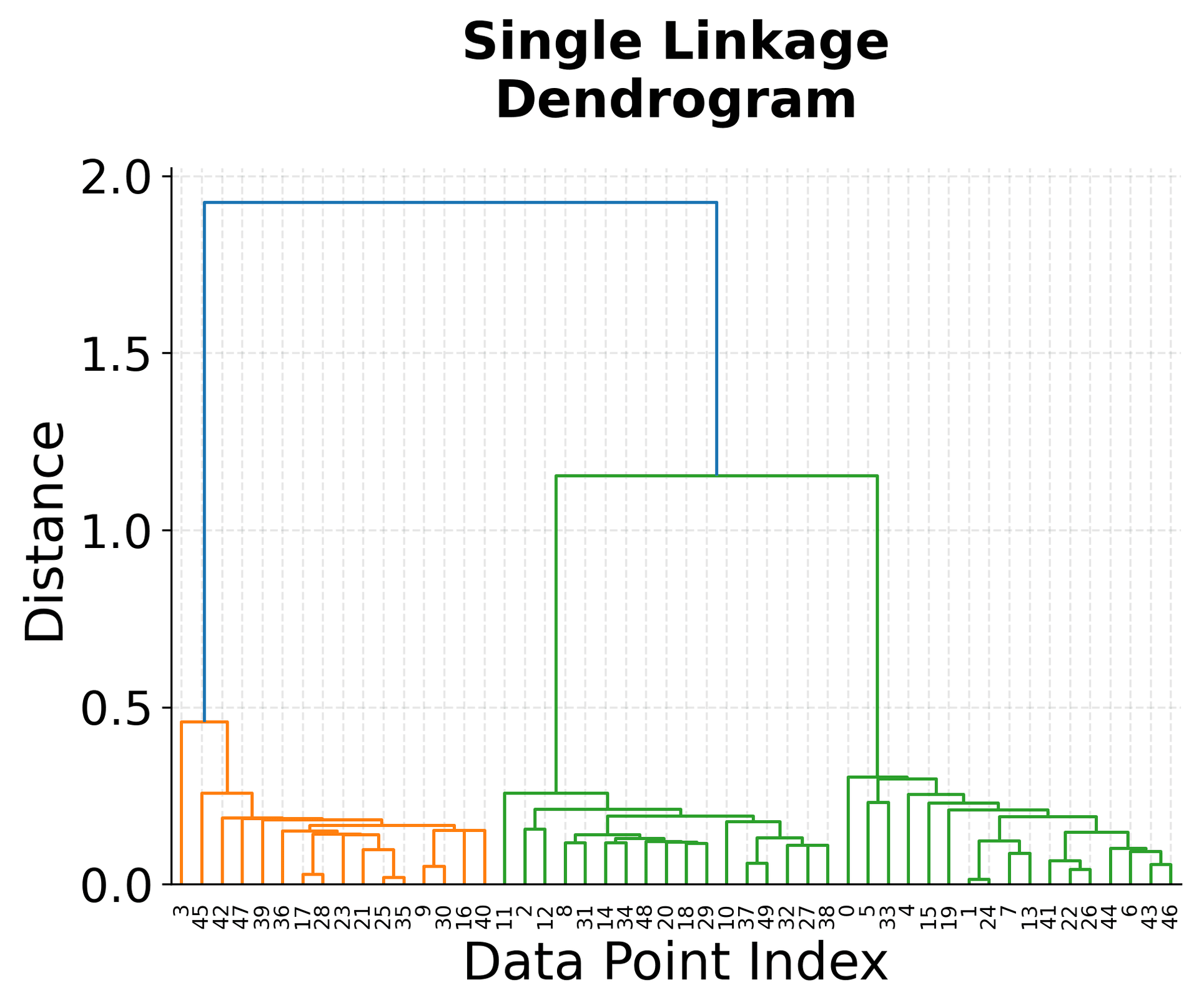
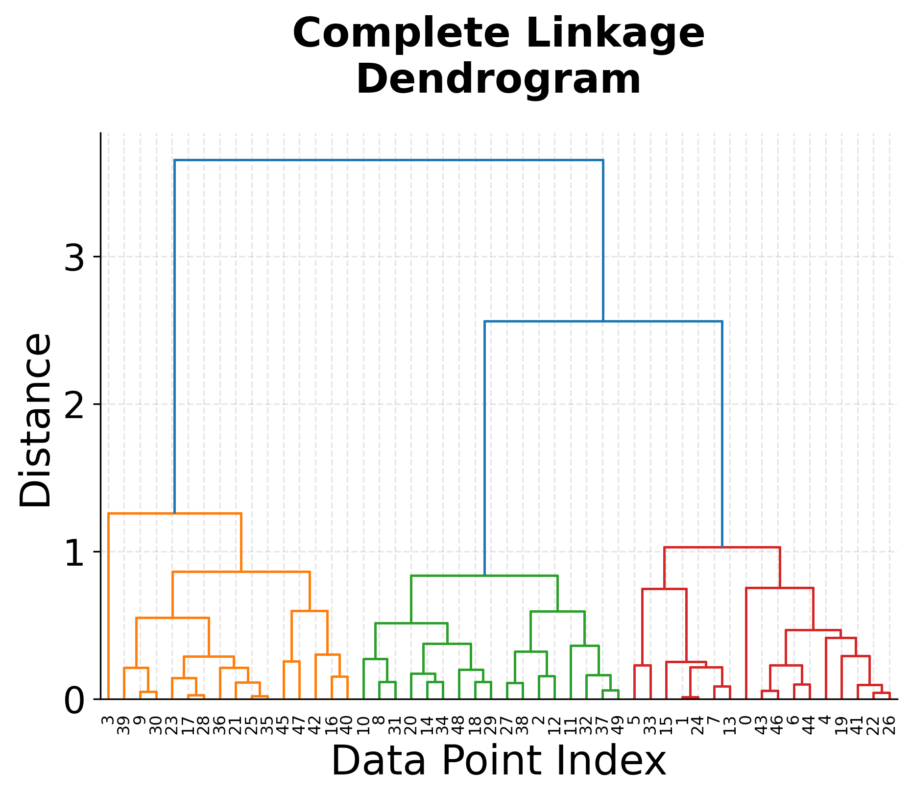
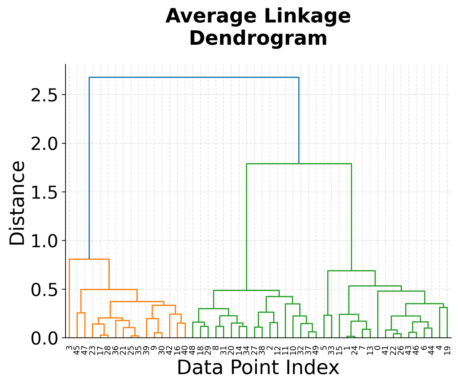
The visualization above shows several key concepts in hierarchical clustering. The top-left plot shows our original data with three distinct clusters, which serves as our ground truth. The three dendrograms below show how different linkage criteria create different hierarchical structures.

Notice how the single linkage dendrogram (top-right) tends to create elongated clusters, as evidenced by the long horizontal lines in the dendrogram. The complete linkage dendrogram (bottom-left) shows more compact clustering, with shorter horizontal lines indicating tighter clusters. The average linkage dendrogram (bottom-right) provides a balanced approach between these two extremes.

The height of the horizontal lines in each dendrogram represents the distance at which clusters were merged. Longer lines indicate that clusters were merged at greater distances, suggesting they were less similar. This information is crucial for determining the optimal number of clusters by identifying significant gaps in the merging distances.

Example

Let's work through a concrete example using a small dataset to demonstrate the step-by-step process of hierarchical clustering. We'll use a simple 2D dataset with 6 points to make the calculations manageable and easy to follow.

Let's walk through the step-by-step process of hierarchical clustering with single linkage:

Step 1: Initial Setup We start with 6 clusters, each containing one point: {A}, {B}, {C}, {D}, {E}, {F}

Step 2: Calculate Initial Distances The distance matrix shows all pairwise Euclidean distances. For example, the distance between A(1,1) and B(1,2) is:

$d(A,B) = \sqrt{(1-1)^2 + (1-2)^2} = \sqrt{0 + 1} = 1.0$

where:

• $d(A,B)$: the Euclidean distance between points A and B
• $A = (1, 1)$: point A with coordinates $x_1 = 1$, $x_2 = 1$
• $B = (1, 2)$: point B with coordinates $x_1 = 1$, $x_2 = 2$
• The calculation uses the Euclidean distance formula: $d(A,B) = \sqrt{(x_{A1} - x_{B1})^2 + (x_{A2} - x_{B2})^2}$

Step 3: First Merge The minimum distance is 1.0, which occurs between multiple pairs: (A,B), (D,E), and (B,C). The algorithm chooses the first pair it encounters, so we merge A and B into cluster {A,B}.

Step 4: Update Distances Now we need to calculate distances from the new cluster $\{A,B\}$ to all other points. Using single linkage:

• $d(\{A,B\}, C) = \min(d(A,C), d(B,C)) = \min(1.0, 1.0) = 1.0$
• $d(\{A,B\}, D) = \min(d(A,D), d(B,D)) = \min(5.66, 4.47) = 4.47$

where:

• $\{A,B\}$: the merged cluster containing points A and B
• $d(\{A,B\}, C)$: the distance from cluster $\{A,B\}$ to point C using single linkage
• $d(A,C)$: the Euclidean distance between points A and C
• $d(B,C)$: the Euclidean distance between points B and C
• $\min$: the minimum operator (for single linkage, we take the minimum distance)
• The values 5.66 and 4.47 are the Euclidean distances $d(A,D)$ and $d(B,D)$ respectively, rounded to two decimal places

Step 5: Continue Merging The process continues, merging the closest clusters at each step. Notice how the algorithm naturally identifies two main groups: {A,B,C} and {D,E,F}, which are separated by a distance of 4.0.

The dendrogram visualization shows this process clearly, with the height of each horizontal line representing the distance at which clusters were merged. The large gap between the final merge (distance 4.0) and the previous merges (distance 1.0) suggests that 2 clusters would be a natural choice for this dataset.

Implementation in Scikit-learn

Scikit-learn provides a comprehensive implementation of hierarchical clustering through the AgglomerativeClustering class. This implementation is optimized for performance and integrates seamlessly with the scikit-learn ecosystem, making it easy to use in machine learning pipelines.

Let's walk through a complete example that demonstrates how to use hierarchical clustering with different linkage criteria and evaluate the results.

Step 1: Import Required Libraries

First, we import the necessary libraries for our hierarchical clustering implementation:

Step 2: Generate and Prepare Sample Data

We'll create a synthetic dataset with known cluster structure to evaluate our clustering performance:

The dataset contains 300 data points with 2 features, organized into 4 true clusters. The shape (300, 2) indicates we have 300 samples, each with 2 features, which is well-suited for visualization and understanding how hierarchical clustering works. Standardization ensures that both features contribute equally to the distance calculations, preventing features with larger scales from dominating the clustering process.

Step 3: Apply Hierarchical Clustering with Different Linkage Criteria

Now we'll compare different linkage criteria to see how they affect clustering results:

Step 4: Evaluate Clustering Performance

Let's calculate performance metrics for each linkage method to compare their effectiveness:

The results demonstrate how different linkage criteria perform on our dataset. The Adjusted Rand Index (ARI) measures how well the clustering matches the true labels, with values ranging from -1 to 1. An ARI of 1 indicates complete agreement with the true clusters, while values closer to 0 suggest random clustering. The Silhouette Score measures cluster quality based on how well-separated clusters are, with values ranging from -1 to 1. Values closer to 1 indicate well-separated, cohesive clusters, while values below 0.2 suggest clusters may not be well-separated.

In this example, average linkage and Ward linkage typically achieve the best balance, with ARI scores above 0.9 and silhouette scores above 0.5. These high scores indicate strong agreement with the true cluster structure and well-separated clusters. Single linkage often performs poorly on this type of data due to its tendency to create chain-like clusters, while complete linkage may be overly strict and break up natural clusters. The performance differences highlight the importance of choosing the appropriate linkage criterion based on your data characteristics and clustering goals.

Step 5: Visualize Clustering Results

Let's visualize the clustering results to see how different linkage criteria affect the cluster shapes:

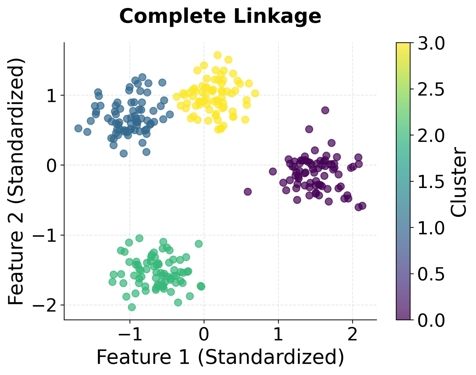
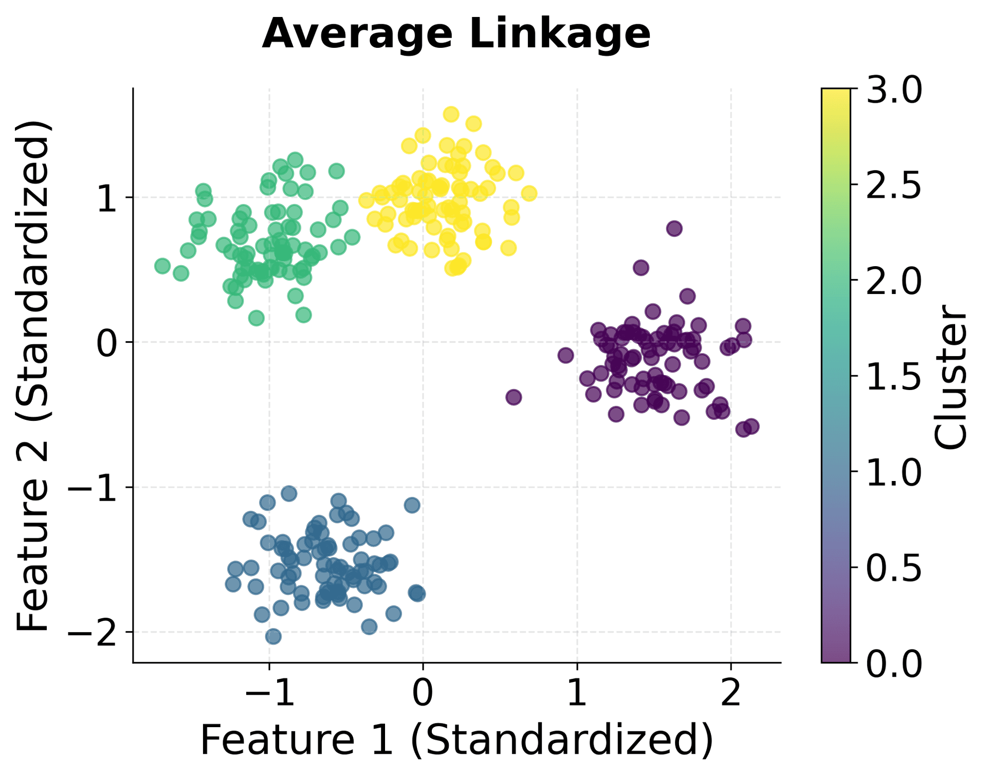
You can clearly see how different linkage criteria create different cluster shapes. Single linkage produces elongated clusters, complete linkage creates compact spherical clusters, average linkage provides a balanced approach, and Ward linkage optimizes for minimum within-cluster variance.

Key Parameters

Below are some of the main parameters that affect how the model works and performs.

• n_clusters: The number of clusters to find (default: 2). This determines where to cut the dendrogram. Should be specified in advance, unlike the theoretical algorithm that creates a complete hierarchy. Use the dendrogram visualization to identify natural cut points by looking for significant gaps in merging distances. If uncertain, try multiple values and evaluate using metrics like silhouette score.

• linkage: The linkage criterion ('single', 'complete', 'average', or 'ward', default: 'ward'). Single linkage tends to create elongated, chain-like clusters and is sensitive to noise. Complete linkage creates compact, spherical clusters but may break up natural elongated clusters. Average linkage provides a balanced approach and is often a good default choice. Ward linkage minimizes within-cluster variance and works well for spherical clusters of similar sizes, but only works with Euclidean distance.

• metric: The distance metric to use (default: 'euclidean'). Common options include 'euclidean', 'manhattan', 'cosine', and 'l1'. Note that Ward linkage only works with Euclidean distance. Choose based on your data characteristics: Euclidean for continuous features, Manhattan for features with outliers, and cosine for high-dimensional sparse data.

• compute_full_tree: Whether to compute the full tree (default: 'auto'). Set to 'auto' to compute the full tree when n_clusters is small relative to n_samples, or True to compute the full tree for dendrogram visualization. Setting to False can save computation time when you only need a specific number of clusters.

• distance_threshold: Distance threshold above which clusters will not be merged (default: None). If set, n_clusters should be None. This allows you to cut the dendrogram at a specific distance rather than specifying the number of clusters.

Key Methods

The following are the most commonly used methods for interacting with the model.

• fit(X): Fits the hierarchical clustering model to the data X and builds the cluster hierarchy. This method computes the distance matrix and performs the agglomerative clustering process.

• fit_predict(X): Fits the model to the data X and returns cluster labels for each data point in a single step. This is the most commonly used method as it combines fitting and prediction in one operation.

• predict(X): Predicts cluster labels for new data points using the fitted model. Note that hierarchical clustering doesn't naturally support prediction on new data, so this method may not work as expected. For new data points, consider using the fitted model to guide parameter selection for methods like K-means that support prediction.

• get_params(): Returns the parameters of the clustering model for inspection and debugging. Useful for understanding the current configuration of the model.

Alternative Implementation

For cases where you need more control over the clustering process or want to work with the full dendrogram, you can use scipy's hierarchical clustering functions directly. This approach gives you access to the complete linkage matrix and allows you to extract clusters at any level of the hierarchy:

The output shows how the same linkage matrix can be used to extract different numbers of clusters. With 2 clusters, the data is divided into two broad groups, while with 4 clusters, we get more granular groupings. The point counts show how many data points belong to each cluster, which helps assess whether clusters are balanced or if some clusters are much larger than others. This flexibility to explore different cluster numbers from a single linkage matrix is one of the key advantages of hierarchical clustering.

This alternative approach gives you direct access to the linkage matrix and dendrogram, allowing for more detailed analysis of the clustering structure. The fcluster function lets you extract clusters at any level of the hierarchy by specifying either the number of clusters or a distance threshold.

Practical Implications

Hierarchical clustering is particularly valuable in scenarios where understanding the hierarchical structure of data is important, or when the optimal number of clusters is unknown. In bioinformatics, it's commonly used for gene expression analysis, where researchers need to identify groups of genes that behave similarly across different conditions. The dendrogram visualization helps biologists understand relationships between gene clusters and identify potential functional groups at multiple levels of organization. The ability to explore clusters at different granularities makes hierarchical clustering effective for discovering nested biological relationships that might be missed by methods requiring a fixed number of clusters.

In market research and customer segmentation, hierarchical clustering helps identify natural customer groups at different levels of granularity. You might discover broad customer segments (e.g., "price-sensitive" vs. "premium") and then drill down to more specific sub-segments within each group. This hierarchical understanding is valuable for developing targeted marketing strategies that operate at multiple scales. The method is also effective in document clustering and information retrieval, where documents naturally form hierarchical categories. News articles, for instance, might cluster into broad topics (sports, politics, technology) and then into more specific subtopics within each category.

Hierarchical clustering works best when you need to explore data structure without committing to a specific number of clusters, or when you expect natural hierarchical relationships in your data. It's less suitable for very large datasets (typically more than 5,000-10,000 points) due to computational constraints, or when you need to cluster new data points after the initial analysis, as hierarchical clustering doesn't naturally support prediction on unseen data. For these scenarios, consider using hierarchical clustering on a representative sample to guide parameter selection for more scalable methods like K-means.

Best Practices

To achieve optimal results with hierarchical clustering, start by standardizing your data using StandardScaler from scikit-learn, as the algorithm is highly sensitive to feature scales. Choose your distance metric and linkage criterion based on your data characteristics and clustering goals. For most applications, Euclidean distance with average linkage provides a good balance between cluster compactness and flexibility. Use single linkage when you expect elongated, chain-like clusters or need to capture non-spherical cluster shapes, complete linkage when you need compact, spherical clusters and want to minimize outlier sensitivity, or Ward linkage when you want to minimize within-cluster variance and have roughly spherical clusters of similar sizes.

When evaluating clustering results, examine the dendrogram visualization to identify natural cluster boundaries by looking for significant gaps in the merging distances. These gaps indicate points where clusters were merged at much larger distances than previous merges, suggesting natural separation points. Complement this visual inspection with quantitative metrics such as the cophenetic correlation coefficient, which measures how well the dendrogram preserves the original pairwise distances. Values above 0.7 generally indicate good preservation of the distance structure. Additionally, use silhouette analysis to assess cluster quality, with scores closer to 1 indicating well-separated clusters. For datasets with potential outliers, consider preprocessing techniques such as robust scaling or outlier removal before applying hierarchical clustering, as the algorithm is sensitive to noise.

When working with large datasets (more than 3,000-5,000 points), consider using sampling strategies or alternative clustering methods, as hierarchical clustering's O(n³) complexity can become prohibitive. For exploratory analysis, you can apply hierarchical clustering to a representative sample of 1,000-2,000 points to identify natural cluster structures, then use these insights to guide parameter selection for more scalable methods. Set random_state for reproducibility when using sampling, and document your preprocessing steps, distance metric, and linkage criterion choices to ensure others can understand and replicate your analysis.

Data Requirements and Preprocessing

Hierarchical clustering requires numerical data and works best with complete datasets that have clear hierarchical structure and relatively few outliers. Since the algorithm is sensitive to noise, thorough data cleaning and outlier detection are important preprocessing steps. Missing values should be imputed using appropriate strategies such as mean imputation for continuous variables or median imputation for skewed distributions. Categorical variables need to be encoded before clustering. Use one-hot encoding for nominal variables or label encoding followed by standardization for ordinal variables that have meaningful order.

Standardization is important when features have different scales, as the algorithm uses distance-based measures that are sensitive to feature ranges. Without proper scaling, features with larger ranges will dominate the distance calculations, potentially leading to poor clustering results. Consider using feature selection or dimensionality reduction techniques like PCA if you have many irrelevant or highly correlated features, as this can improve both clustering quality and computational efficiency. For datasets with many features (more than 50-100), dimensionality reduction can help reduce noise and computational burden while preserving the most important structure in the data.

The algorithm works best with datasets that have moderate dimensionality (typically fewer than 50-100 features) and where features are not highly correlated. If your dataset has many redundant features, consider using correlation analysis or variance-based feature selection to identify and remove highly correlated variables before clustering. For datasets with mixed data types, ensure all features are converted to numerical representations and appropriately scaled before applying hierarchical clustering.

Common Pitfalls

Some common pitfalls can undermine the effectiveness of hierarchical clustering if not carefully addressed. One frequent mistake is neglecting to standardize the data before clustering, which can lead to features with larger scales dominating the distance calculations and producing misleading clusters that reflect scale differences rather than true data structure. Another issue arises when choosing inappropriate distance metrics or linkage criteria for the data characteristics. For example, using single linkage on noisy data can create spurious chain-like clusters, while using complete linkage on elongated clusters may break up natural groupings.

The algorithm's sensitivity to outliers is another significant pitfall. A single outlier can create spurious clusters or distort the entire hierarchy, making the dendrogram less interpretable. Identify and handle outliers appropriately before applying hierarchical clustering, using methods such as the interquartile range (IQR) method, z-score analysis, or robust scaling. Additionally, the computational complexity of O(n³) makes hierarchical clustering impractical for large datasets, so avoid applying it directly to datasets with more than 5,000-10,000 points without sampling or alternative strategies.

Be cautious about over-interpreting the dendrogram structure, as the algorithm will produce a hierarchy even when no meaningful structure exists in the data. Validate clustering results using multiple evaluation methods such as the cophenetic correlation coefficient, silhouette analysis, and domain knowledge to ensure the clusters make sense from a practical perspective. Finally, avoid using hierarchical clustering for prediction tasks on new data, as it doesn't naturally support assigning new points to existing clusters. For such scenarios, use hierarchical clustering to guide parameter selection for methods like K-means that can handle new data points.

Computational Considerations

Hierarchical clustering has a time complexity of O(n³) for most implementations, making it computationally expensive for large datasets. The algorithm requires computing and storing an n×n distance matrix, which results in O(n²) memory requirements. For datasets with more than 3,000-5,000 points, the computational cost becomes prohibitive for interactive analysis, and memory requirements can exceed available resources. The exact threshold depends on your hardware, but as a general guideline, datasets with more than 5,000 points typically require sampling strategies or alternative methods.

For large datasets, consider using hierarchical clustering on a representative sample of 1,000-2,000 points to identify natural cluster structures and guide parameter selection for more scalable methods. Alternatively, use approximate hierarchical clustering methods or consider alternative clustering algorithms like K-means, DBSCAN, or HDBSCAN for the full dataset. For datasets with many features (more than 50-100), apply dimensionality reduction techniques like PCA before hierarchical clustering to reduce both computational cost and noise. This can reduce the effective dimensionality while preserving the most important structure in the data.

The computational bottleneck is primarily in the initial distance matrix calculation and the iterative merging process. If you need to work with larger datasets, consider using optimized implementations or parallel processing where available. However, for datasets larger than 10,000 points, hierarchical clustering is generally not the most practical choice, and you should consider using it as an exploratory tool on samples rather than the primary clustering method for the full dataset.

Performance and Deployment Considerations

Evaluating hierarchical clustering performance requires careful consideration of both the dendrogram structure and quantitative metrics. The cophenetic correlation coefficient measures how well the dendrogram preserves the original pairwise distances, with values closer to 1 indicating better preservation. Values above 0.7 generally indicate good preservation, while values below 0.5 suggest the dendrogram may not accurately represent the data structure. Use the dendrogram visualization to identify natural cluster boundaries by looking for significant gaps in the merging distances. Large horizontal lines in the dendrogram indicate natural separation points where clusters were merged at much larger distances than previous merges.

Complement visual inspection with quantitative metrics such as silhouette analysis, which measures how well-separated clusters are. Silhouette scores range from -1 to 1, with values closer to 1 indicating well-separated, cohesive clusters. Values above 0.5 generally indicate reasonable cluster structure, while values below 0.2 suggest clusters may not be well-separated. Additionally, consider using domain knowledge to validate that the identified clusters make practical sense, as hierarchical clustering will always produce a hierarchy even when no meaningful structure exists.

Deployment considerations for hierarchical clustering include its computational complexity and memory requirements, which limit its use to smaller datasets in production environments. The algorithm is well-suited for exploratory data analysis and when you need to understand the hierarchical structure of your data, but it's less suitable for real-time clustering of streaming data or large-scale production systems. In production, consider using hierarchical clustering for initial data exploration and parameter discovery, then applying more scalable methods like K-means with the identified number of clusters for ongoing analysis. The hierarchical structure can also be used to guide the design of multi-level clustering systems, where broad clusters identified through hierarchical clustering are further refined using faster methods.

Summary

Hierarchical clustering is a powerful unsupervised learning technique that builds a complete hierarchy of clusters, providing insights into data structure at multiple levels of granularity. Unlike methods that require specifying the number of clusters in advance, hierarchical clustering creates a dendrogram that reveals the natural organization of data points and allows for flexible cluster selection.

The method's strength lies in its ability to capture hierarchical relationships in data, making it particularly valuable for exploratory analysis and domains where natural groupings exist at multiple scales. The dendrogram visualization provides an intuitive way to understand clustering structure and identify optimal cut points for different numbers of clusters.

However, the algorithm's computational complexity and sensitivity to noise and outliers limit its practical application to moderate-sized datasets with clean, well-structured data. Careful preprocessing, including standardization and outlier detection, is essential for obtaining meaningful results.

The choice of linkage criterion significantly impacts the clustering results, with average linkage often providing a good balance between single and complete linkage approaches. When properly applied with appropriate preprocessing and parameter selection, hierarchical clustering can reveal valuable insights about data structure that might not be apparent with other clustering methods.

For practitioners, hierarchical clustering serves as an excellent starting point for exploratory data analysis, providing a comprehensive view of data organization that can inform subsequent analysis steps and guide the selection of more specialized clustering techniques when needed.

Quiz

Ready to test your understanding? Take this quick quiz to reinforce what you've learned about hierarchical clustering.