InteractivePCA (Principal Component Analysis): Complete Guide with Mathematical Foundation & Implementation

PCA (Principal Component Analysis)

Concept

Principal Component Analysis (PCA) is a dimensionality reduction technique that transforms high-dimensional data into a lower-dimensional space while preserving as much of the original information as possible. The core idea is straightforward: find the directions where your data varies the most. Think of it like finding the best camera angles to photograph a sculpture. Some angles capture more information about the shape than others. PCA identifies these "best angles" mathematically and lets you represent your data using just the most informative views.

What makes PCA different from simply picking a few features to keep? Instead of choosing existing features, PCA creates entirely new features by combining the original ones. Each new feature, called a principal component, is a weighted sum of all the original features. The first principal component points in the direction of maximum variance. The second principal component points in the direction of maximum remaining variance while being perpendicular to the first. This pattern continues for all components.

PCA is unsupervised, meaning it doesn't need any labels or target variables. It looks purely at the structure of the input data itself. This makes it versatile for many tasks, from visualization to preprocessing to compression.

The method works best when your features are correlated, when they have linear relationships. If age and income both increase together in your data, PCA can capture this pattern in a single component rather than keeping both features separate. By finding these underlying patterns, PCA often reduces dimensionality dramatically while retaining most of the important information. This leads to faster computations, lower storage needs, and sometimes better model performance by filtering out noise.

Advantages

PCA has several strengths that explain its popularity:

Mathematical soundness: PCA has a clear objective (maximize variance) and a closed-form solution through eigenvalue decomposition. There's no iterative optimization that might fail to converge, and no hyperparameters to tune for the core algorithm.

Computational efficiency: For moderate-sized datasets, PCA runs quickly. The eigenvalue decomposition required to find components is well-studied, and modern linear algebra libraries make it efficient. For large datasets, approximation methods like randomized SVD maintain good performance.

Interpretability: Each principal component is a linear combination of the original features. We can examine the coefficients (loadings) to understand which original features contribute most to each component. This makes PCA valuable for both preprocessing and understanding data structure.

Disadvantages

PCA has limitations that practitioners should understand:

Linear assumptions: PCA only captures linear relationships between variables. If your data has non-linear patterns or complex interactions, PCA may miss important structure. For such cases, consider non-linear alternatives like kernel PCA or manifold learning methods.

Scale sensitivity: PCA is sensitive to the scale of input variables. Variables with larger numerical ranges will dominate the principal components, potentially masking patterns in smaller-scale variables. Standardization (mean centering and scaling to unit variance) is typically required before applying PCA, though this preprocessing can alter the interpretation of results.

Variance as importance: PCA assumes that directions of maximum variance are most important. While this often holds true, there are cases where maximum variance directions may not be most relevant for the task. In supervised learning, for example, directions that best separate classes might not align with maximum variance directions.

Formula

Now let's build the mathematics of PCA step by step, starting from basic concepts you already know and working toward the full algorithm. The journey from variance to principal components is more natural than you might expect.

Starting with Variance

Think about a single variable, like the heights of people in a dataset. How spread out are the values? Variance answers this question:

$\text{Var}(x) = \frac{1}{n-1} \sum_{i=1}^{n} (x_i - \bar{x})^2$

Here $\bar{x}$ is the mean (average) of $x$. For each data point, we calculate how far it is from the mean, square that distance, and average all the squared distances. The squaring ensures that deviations above and below the mean both contribute positively to the total spread.

Now consider two variables, height $x$ and weight $y$. Do they vary together? Covariance measures this:

$\text{Cov}(x,y) = \frac{1}{n-1} \sum_{i=1}^{n} (x_i - \bar{x})(y_i - \bar{y})$

If tall people tend to be heavier, then when $x_i - \bar{x}$ is positive (taller than average), $y_i - \bar{y}$ tends to be positive too (heavier than average). Multiplying these together gives positive products, so the covariance is positive. If the variables move in opposite directions, covariance is negative. If they're unrelated, positive and negative products cancel out, giving covariance near zero.

The Covariance Matrix

When you have many variables, say $p$ of them, you need to track all pairwise relationships. The covariance matrix $\mathbf{C}$ does exactly this:

$\mathbf{C} = \frac{1}{n-1} \mathbf{X}^T \mathbf{X}$

Here $\mathbf{X}$ is your data matrix with $n$ rows (observations) and $p$ columns (variables). We assume you've already mean-centered the data, meaning you subtracted the mean from each column so each variable has mean zero.

What does this matrix contain? The diagonal elements are the variances of each individual variable. The off-diagonal elements are the covariances between pairs of variables. So if you have three variables, your covariance matrix looks like:

This matrix is symmetric because $\text{Cov}(x_i,x_j) = \text{Cov}(x_j,x_i)$. The covariance matrix captures all the linear relationships in your data in one compact object.

Finding Principal Components

Here's the key question PCA answers: in which direction does the data vary the most?

Imagine drawing a line through your data cloud. You can project each point onto this line by dropping a perpendicular from the point to the line. The projected points form a one-dimensional dataset on the line. Some lines will give you spread-out projections (high variance), others will give you bunched-up projections (low variance). PCA finds the line that maximizes this variance.

Mathematically, a direction is a unit vector $\mathbf{w}$ (length 1). When you project your data $\mathbf{X}$ onto $\mathbf{w}$, you get $\mathbf{X}\mathbf{w}$. The variance of this projection is:

$\text{Var}(\mathbf{X}\mathbf{w}) = \mathbf{w}^T \mathbf{C} \mathbf{w}$

This compact formula says: the variance in direction $\mathbf{w}$ equals $\mathbf{w}^T \mathbf{C} \mathbf{w}$, where $\mathbf{C}$ is the covariance matrix. To find the direction of maximum variance, we need to maximize $\mathbf{w}^T \mathbf{C} \mathbf{w}$ subject to the constraint that $\mathbf{w}$ has unit length ($\mathbf{w}^T \mathbf{w} = 1$).

Why the constraint? Without it, we could make the variance arbitrarily large just by making $\mathbf{w}$ longer. Requiring unit length keeps the problem well-defined.

This is a constrained optimization problem. We solve it using Lagrange multipliers, a technique you may remember from calculus. We form the Lagrangian:

$\mathcal{L} = \mathbf{w}^T \mathbf{C} \mathbf{w} - \lambda(\mathbf{w}^T \mathbf{w} - 1)$

The term $\lambda(\mathbf{w}^T \mathbf{w} - 1)$ enforces our constraint. Taking the derivative with respect to $\mathbf{w}$ and setting it to zero:

$\frac{\partial \mathcal{L}}{\partial \mathbf{w}} = 2\mathbf{C}\mathbf{w} - 2\lambda\mathbf{w} = 0$

Simplifying by dividing by 2:

$\mathbf{C}\mathbf{w} = \lambda\mathbf{w}$

This is the eigenvalue equation. The solutions $\mathbf{w}$ are the eigenvectors of $\mathbf{C}$, and the values $\lambda$ are the eigenvalues. What does this mean? The principal components are eigenvectors of the covariance matrix. The variance along each principal component is the corresponding eigenvalue. Larger eigenvalues mean more variance in that direction.

The Complete PCA Transformation

Once you've found all the eigenvectors, you can transform your data into the new coordinate system:

$\mathbf{Y} = \mathbf{X}\mathbf{W}$

Here $\mathbf{W}$ is a matrix whose columns are the eigenvectors of $\mathbf{C}$. Each column is a principal component (a direction of variance). The matrix $\mathbf{Y}$ contains your data in the new coordinate system. Each column of $\mathbf{Y}$ is a principal component score, telling you the position of each observation along that component.

The eigenvalues tell you how much variance each component captures. To find what proportion of total variance the $k$-th component explains:

$\frac{\lambda_k}{\sum_{j=1}^{p} \lambda_j}$

If the first eigenvalue is $\lambda_1 = 5$ and the sum of all eigenvalues is $10$, then the first principal component explains $5/10 = 50\%$ of the total variance. This helps you decide how many components to keep. If the first three components explain 95% of variance, you might drop the rest.

Mathematical Properties

PCA has several mathematical properties worth knowing:

Orthogonality: Principal components are perpendicular (orthogonal) to each other. This means they capture different, non-overlapping patterns in the data. Each component adds new information rather than repeating what previous components captured.

Variance preservation: The total variance in the original data equals the sum of all eigenvalues. When you keep the first $k$ components, you capture the maximum possible variance among all sets of $k$ orthogonal directions. No other choice of $k$ perpendicular directions would capture more variance.

Optimality for reconstruction: When you project your data onto $k$ components and reconstruct it back in the original space, PCA minimizes the mean squared reconstruction error. Among all possible $k$-dimensional linear projections, PCA provides the best approximation to the original data.

Visualizing PCA

The mathematics is clearer when you see it in action. Let's visualize PCA on a simple two-dimensional dataset where we can actually see what's happening.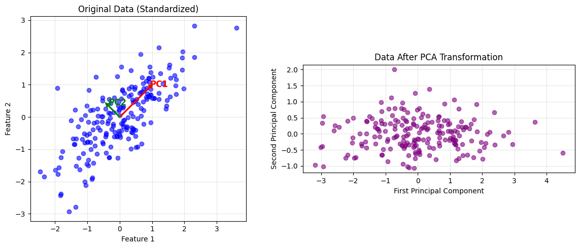

Example

Let's work through PCA by hand on a tiny dataset. This will make the abstract formulas concrete. We'll calculate each step explicitly so you see exactly how the algorithm works.

Suppose we have four observations of two variables:

$\mathbf{X} = \begin{bmatrix} 1 & 2 \\ 2 & 3 \\ 3 & 4 \\ 4 & 5 \end{bmatrix}$

Each row is an observation, each column is a variable. Notice the strong relationship: the second variable is always one more than the first.

Step 1: Mean Centering

PCA requires mean-centered data. First, calculate the mean of each variable:

• Mean of variable 1: $\bar{x}_1 = \frac{1+2+3+4}{4} = 2.5$
• Mean of variable 2: $\bar{x}_2 = \frac{2+3+4+5}{4} = 3.5$

Now subtract these means from each observation:

$\mathbf{X}_{\text{centered}} = \begin{bmatrix} 1-2.5 & 2-3.5 \\ 2-2.5 & 3-3.5 \\ 3-2.5 & 4-3.5 \\ 4-2.5 & 5-3.5 \end{bmatrix} = \begin{bmatrix} -1.5 & -1.5 \\ -0.5 & -0.5 \\ 0.5 & 0.5 \\ 1.5 & 1.5 \end{bmatrix}$

Each column now has mean zero. The data is centered at the origin.

Step 2: Calculate the Covariance Matrix

Next, compute the covariance matrix using $\mathbf{C} = \frac{1}{n-1} \mathbf{X}_{\text{centered}}^T \mathbf{X}_{\text{centered}}$. With $n=4$ observations, we divide by $n-1=3$:

$\mathbf{C} = \frac{1}{3} \begin{bmatrix} -1.5 & -0.5 & 0.5 & 1.5 \\ -1.5 & -0.5 & 0.5 & 1.5 \end{bmatrix} \begin{bmatrix} -1.5 & -1.5 \\ -0.5 & -0.5 \\ 0.5 & 0.5 \\ 1.5 & 1.5 \end{bmatrix}$

Let's calculate element by element:

• $C_{11} = \frac{1}{3}[(-1.5)^2 + (-0.5)^2 + (0.5)^2 + (1.5)^2] = \frac{1}{3}[2.25 + 0.25 + 0.25 + 2.25] = \frac{5}{3} \approx 1.67$

This is the variance of variable 1.

• $C_{12} = C_{21} = \frac{1}{3}[(-1.5)(-1.5) + (-0.5)(-0.5) + (0.5)(0.5) + (1.5)(1.5)] = \frac{1}{3}[2.25 + 0.25 + 0.25 + 2.25] = \frac{5}{3} \approx 1.67$

This is the covariance between variables 1 and 2. It's positive and large, confirming the strong positive relationship we saw.

• $C_{22} = \frac{1}{3}[(-1.5)^2 + (-0.5)^2 + (0.5)^2 + (1.5)^2] = \frac{5}{3} \approx 1.67$

This is the variance of variable 2.

The covariance matrix is:

$\mathbf{C} = \begin{bmatrix} 1.67 & 1.67 \\ 1.67 & 1.67 \end{bmatrix}$

Notice that the covariance equals the variances. This happens when two variables are perfectly correlated, as ours nearly are.

Step 3: Find Eigenvalues and Eigenvectors

Now we solve the eigenvalue equation $\mathbf{C}\mathbf{w} = \lambda\mathbf{w}$. Rearranging, we get $(\mathbf{C} - \lambda\mathbf{I})\mathbf{w} = 0$, where $\mathbf{I}$ is the identity matrix.

For non-trivial solutions (where $\mathbf{w} \neq 0$), the matrix $\mathbf{C} - \lambda\mathbf{I}$ must be singular, meaning its determinant equals zero. This gives the characteristic equation:

$\det(\mathbf{C} - \lambda\mathbf{I}) = 0$

Substituting our covariance matrix:

$\det\begin{bmatrix} 1.67-\lambda & 1.67 \\ 1.67 & 1.67-\lambda \end{bmatrix} = 0$

The determinant of a 2×2 matrix $\begin{bmatrix} a & b \\ c & d \end{bmatrix}$ is $ad - bc$, so:

$(1.67-\lambda)(1.67-\lambda) - (1.67)(1.67) = 0$

$(1.67-\lambda)^2 - (1.67)^2 = 0$

This factors as a difference of squares:

$[(1.67-\lambda) - 1.67][(1.67-\lambda) + 1.67] = 0$

$(-\lambda)(3.34 - \lambda) = 0$

So $\lambda = 0$ or $\lambda = 3.34$. These are our two eigenvalues.

Now find the eigenvector for each eigenvalue.

For $\lambda_1 = 3.34$:

Substitute into $(\mathbf{C} - \lambda\mathbf{I})\mathbf{w} = 0$:

$\begin{bmatrix} 1.67-3.34 & 1.67 \\ 1.67 & 1.67-3.34 \end{bmatrix}\begin{bmatrix} w_1 \\ w_2 \end{bmatrix} = \begin{bmatrix} 0 \\ 0 \end{bmatrix}$

$\begin{bmatrix} -1.67 & 1.67 \\ 1.67 & -1.67 \end{bmatrix}\begin{bmatrix} w_1 \\ w_2 \end{bmatrix} = \begin{bmatrix} 0 \\ 0 \end{bmatrix}$

The first row gives $-1.67w_1 + 1.67w_2 = 0$, which simplifies to $w_1 = w_2$. So the eigenvector has equal components. To make it unit length, we need $w_1^2 + w_2^2 = 1$. Since $w_1 = w_2$, we have $2w_1^2 = 1$, so $w_1 = \frac{1}{\sqrt{2}}$:

$\mathbf{w}_1 = \begin{bmatrix} \frac{1}{\sqrt{2}} \\ \frac{1}{\sqrt{2}} \end{bmatrix} \approx \begin{bmatrix} 0.707 \\ 0.707 \end{bmatrix}$

This is the first principal component. It points equally in both variable directions, capturing their shared variation.

For $\lambda_2 = 0$:

$\begin{bmatrix} 1.67 & 1.67 \\ 1.67 & 1.67 \end{bmatrix}\begin{bmatrix} w_1 \\ w_2 \end{bmatrix} = \begin{bmatrix} 0 \\ 0 \end{bmatrix}$

This gives $1.67w_1 + 1.67w_2 = 0$, so $w_1 = -w_2$. With unit length:

$\mathbf{w}_2 = \begin{bmatrix} \frac{1}{\sqrt{2}} \\ -\frac{1}{\sqrt{2}} \end{bmatrix} \approx \begin{bmatrix} 0.707 \\ -0.707 \end{bmatrix}$

This is the second principal component. It points in the direction perpendicular to the first. Note that $\lambda_2 = 0$ means this direction has zero variance, which makes sense because our data lies along a perfect line.

Step 4: Transform the Data

Finally, project the data onto the principal components using $\mathbf{Y} = \mathbf{X}_{\text{centered}}\mathbf{W}$:

$\mathbf{Y} = \begin{bmatrix} -1.5 & -1.5 \\ -0.5 & -0.5 \\ 0.5 & 0.5 \\ 1.5 & 1.5 \end{bmatrix} \begin{bmatrix} 0.707 & 0.707 \\ 0.707 & -0.707 \end{bmatrix}$

Let's compute a few entries to see the pattern:

• $Y_{11} = (-1.5)(0.707) + (-1.5)(0.707) = -1.061 - 1.061 = -2.121$
• $Y_{12} = (-1.5)(0.707) + (-1.5)(-0.707) = -1.061 + 1.061 = 0$
• $Y_{21} = (-0.5)(0.707) + (-0.5)(0.707) = -0.354 - 0.354 = -0.707$
• $Y_{22} = (-0.5)(0.707) + (-0.5)(-0.707) = -0.354 + 0.354 = 0$

Following this pattern for all rows:

$\mathbf{Y} = \begin{bmatrix} -2.121 & 0 \\ -0.707 & 0 \\ 0.707 & 0 \\ 2.121 & 0 \end{bmatrix}$

Look at what happened. The second column (second principal component) is all zeros. This makes perfect sense. Our original data was perfectly correlated, lying along a single line. All the variance is captured by the first principal component (the direction along that line). The second principal component, perpendicular to that line, has no variance at all.

If you wanted to reduce dimensionality, you could keep only the first column and represent your data in one dimension instead of two, losing zero information.

Implementation in Scikit-learn

Now that you understand the theory, let's see how to use PCA in practice. Scikit-learn handles all the computational details, making PCA easy to apply to real datasets.

Key Parameters and Methods

Scikit-learn's PCA offers several useful parameters:

n_components: How many components to keep. You can specify this as:

• An integer (e.g., n_components=3 keeps the first three components)
• A float between 0 and 1 (e.g., n_components=0.95 keeps enough components to explain 95% of variance)
• 'mle' for automatic selection using maximum likelihood estimation

whiten: Whether to scale components to have unit variance. This is useful when you plan to use the transformed data in algorithms that assume features have similar scales.

svd_solver: Which algorithm to use for the underlying singular value decomposition. Options include 'auto' (chooses based on data size), 'full' (exact SVD), 'arpack' (iterative for sparse data), and 'randomized' (fast approximation for large datasets).

Practical Implications

PCA works best on high-dimensional data with correlated features. Here's when and how to use it effectively:

Data Preprocessing for Machine Learning

PCA is often used before training machine learning models. Reducing dimensionality can improve performance, reduce overfitting, and speed up training. This matters most for algorithms that struggle with many dimensions, like k-nearest neighbors. It's also helpful when you have more features than observations, a situation that causes problems for many models.

Exploratory Data Analysis

PCA reveals structure in high-dimensional data. The principal components show the main patterns of variation. The loadings (weights on original features) tell you which features matter most for each component. This can uncover relationships you wouldn't see in the raw features. For example, you might discover that income, education, and occupation all load heavily on one component, suggesting an underlying "socioeconomic status" factor.

Data Compression and Storage

When storage or transmission is expensive, PCA can compress data while keeping most information. In image processing, you might reduce thousands of pixels to a few dozen principal components. The images look nearly identical but take far less space.

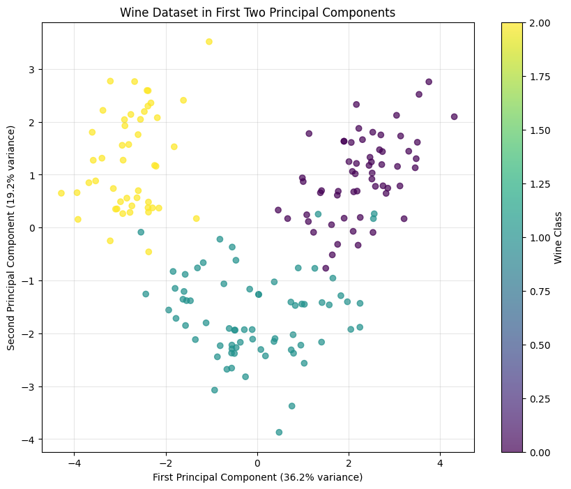
Visualization

PCA lets you plot high-dimensional data in 2D or 3D. Project onto the first two or three components and make a scatter plot. You lose information (everything not in those components), but you gain the ability to see patterns like clusters or outliers. This is invaluable for understanding your data before modeling.

Noise Reduction

Later principal components often capture mostly noise rather than signal. By keeping only the first few components, you filter noise while preserving structure. This is useful in signal processing and with noisy measurements.

When to Use PCA (and When Not To)

Use PCA when:

• You have linear relationships between features
• You want to preserve global variance patterns
• You need interpretable components
• Computational efficiency matters

Consider alternatives when:

• Your data has non-linear structure (try kernel PCA or autoencoders)
• You need to preserve local neighborhoods (try t-SNE or UMAP)
• You're doing supervised learning and class separation matters more than variance (try Linear Discriminant Analysis)

Data Requirements

Standardize your data before applying PCA by subtracting the mean and dividing by standard deviation for each feature. Without standardization, features with large numerical ranges will dominate the components regardless of their actual importance.

PCA assumes that variance correlates with importance. This assumption works well for many tasks, but not universally. In some datasets, informative signals may have low variance while high-variance directions contain primarily noise.

Computational Considerations

PCA scales reasonably well but can be slow on very large datasets. For millions of samples or thousands of features, use the randomized SVD solver for faster (approximate) results. For datasets too large to fit in memory, try incremental PCA, which processes data in batches.

Summary

Principal Component Analysis finds the directions of maximum variance in data and uses them to create a simpler representation. It is one of the most widely used dimensionality reduction techniques due to its mathematical soundness and practical utility.

The strength of PCA lies in its transparency. Principal components are linear combinations of original features, making them interpretable. The eigenvalues quantify exactly how much variance each component captures, providing clear guidance on dimensionality reduction. The algorithm has a closed-form solution with no iterative optimization or core hyperparameters to tune.

PCA has limitations. It assumes linear relationships, so it may miss non-linear patterns. It is sensitive to feature scales, requiring standardization. It assumes high-variance directions are important, which may not hold for supervised learning tasks where class separation can matter more than overall variance.

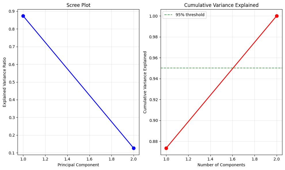
Despite these limitations, PCA remains valuable in data science for exploratory analysis, visualization, preprocessing, and compression. When applied appropriately (with standardization, scree plot analysis, and consideration of whether variance indicates importance for the specific task), PCA effectively reveals patterns and simplifies complex datasets.