InteractiveHDBSCAN Clustering: Complete Guide to Hierarchical Density-Based Clustering with Automatic Cluster Selection

HDBSCAN (Hierarchical Density-Based Spatial Clustering of Applications with Noise)

HDBSCAN (Hierarchical Density-Based Spatial Clustering of Applications with Noise) is an advanced clustering algorithm that extends the popular DBSCAN method by incorporating hierarchical clustering principles. Unlike traditional clustering algorithms that require you to specify the number of clusters beforehand, HDBSCAN automatically determines the optimal number of clusters while being robust to noise and outliers.

The algorithm works by building a hierarchy of clusters based on density, allowing it to identify clusters of varying densities and shapes. This makes HDBSCAN particularly powerful for real-world datasets where clusters may have different characteristics or where the number of clusters is unknown. The hierarchical approach also enables the algorithm to handle nested clusters and provides a more nuanced understanding of the data structure.

HDBSCAN distinguishes itself from other clustering methods by combining the density-based approach of DBSCAN with the hierarchical clustering framework. While DBSCAN treats all points within a density threshold equally, HDBSCAN creates a hierarchy that allows for more sophisticated cluster selection and provides stability across different parameter settings.

Advantages

HDBSCAN offers several key advantages that make it particularly valuable for complex clustering tasks. First, the algorithm automatically determines the number of clusters without requiring prior knowledge, which is especially beneficial when exploring unknown datasets. This automatic cluster selection is based on the stability of clusters across different density thresholds, providing a principled approach to cluster identification.

The hierarchical nature of HDBSCAN allows it to handle clusters of varying densities within the same dataset. Unlike k-means or other centroid-based methods that assume spherical clusters, HDBSCAN can identify clusters with arbitrary shapes and sizes. This flexibility makes it particularly suitable for real-world data where clusters may have complex geometries or varying densities.

Another significant advantage is HDBSCAN's robustness to noise and outliers. The algorithm explicitly identifies noise points, allowing you to focus on the meaningful clusters while being aware of potentially problematic data points. This noise handling is particularly valuable in domains like anomaly detection or when working with messy, real-world datasets.

Disadvantages

Despite its strengths, HDBSCAN has several limitations that should be considered when choosing a clustering algorithm. The algorithm can be computationally expensive, especially for large datasets, as it requires building a complete hierarchy and computing mutual reachability distances between all points. This computational complexity can make HDBSCAN impractical for very large datasets or real-time applications.

HDBSCAN's performance is sensitive to the choice of hyperparameters, particularly the min_cluster_size and min_samples parameters. While the algorithm provides some guidance for parameter selection, choosing inappropriate values can lead to poor clustering results. The parameter sensitivity means that some experimentation and domain knowledge are often required to achieve optimal results.

The algorithm also struggles with high-dimensional data due to the curse of dimensionality. As the number of dimensions increases, the concept of density becomes less meaningful, and the distance-based approach may not capture the true structure of the data. This limitation is common to most density-based clustering methods and may require dimensionality reduction techniques as a preprocessing step.

Formula

To understand how HDBSCAN works, we need to explore how it measures density, builds relationships between points, and selects meaningful clusters. The algorithm adapts to varying densities across the dataset, which is a capability that many traditional clustering methods lack. Let's build this understanding step by step, starting with the fundamental question: how do we measure local density in a way that works for clusters of different sizes and shapes?

Understanding Local Density Through Neighborhoods

Imagine you're standing in a crowded city square. If you look around and see many people nearby, you're in a dense area. If you see only a few people far away, you're in a sparse area. HDBSCAN uses a similar intuition, but formalizes it mathematically through the concept of neighborhoods.

For each point in the dataset, HDBSCAN asks: "How far do I need to look to find k other points?" This distance tells us about the local density around that point. Points in dense clusters will have nearby neighbors, while isolated points or noise will need to look much farther.

This idea is captured by the core distance, which measures the distance from a point to its k-th nearest neighbor:

where:

• $\text{core}_k(x)$: core distance of point $x$ (distance to its k-th nearest neighbor)
• $d(x, \text{kNN}(x))$: Euclidean distance from point $x$ to its k-th nearest neighbor
• $k$: the min_samples parameter, which controls how many neighbors we require (typically set to the minimum number of samples in a neighborhood for a point to be considered a core point)
• $x$: a data point in the dataset
• $\text{kNN}(x)$: the k-th nearest neighbor of point $x$

The core distance is small for points in dense regions and large for isolated points. This gives us a local measure of density that adapts to each point's immediate surroundings, rather than using a single global threshold like DBSCAN does.

Creating a Density-Aware Distance Metric

Now comes the key insight: when measuring distances between points, we should account for the density of the regions they inhabit. Two points in a dense cluster should be considered "close" even if their Euclidean distance is moderate, because they're both in a region of high density. Conversely, two points in sparse regions should be considered "distant" even if they're relatively close in Euclidean space, because they're both in low-density areas.

This leads to the mutual reachability distance, which adjusts distances based on local density:

where:

• $d_{\text{mreach}}(x,y)$: mutual reachability distance between points $x$ and $y$ (a density-aware distance metric)
• $\text{core}_k(x)$: core distance of point $x$ (distance to its k-th nearest neighbor)
• $\text{core}_k(y)$: core distance of point $y$ (distance to its k-th nearest neighbor)
• $d(x,y)$: Euclidean distance between points $x$ and $y$
• $k$: the min_samples parameter (same as in the core distance calculation)
• $x, y$: two data points in the dataset

This formula ensures that the distance between two points is at least as large as the core distance of either point. Here's why this matters: if either point is in a sparse region (large core distance), the mutual reachability distance will reflect that sparsity, effectively "stretching" the distance between sparse regions. Points in dense regions (small core distances) remain close to each other, while points in sparse regions become farther apart.

This density-aware distance metric is the foundation that allows HDBSCAN to handle clusters of varying densities. By transforming the original distance space into a mutual reachability space, we create a representation where dense clusters are well-separated from sparse regions, making cluster identification more robust.

Building a Hierarchical Structure

With our density-aware distances, we can now construct a hierarchical representation of the data. HDBSCAN builds a minimum spanning tree (MST) using the mutual reachability distances. The MST connects all points using the minimum total edge weight, creating a tree structure where each edge represents a connection between points.

The MST construction finds the spanning tree $T$ that minimizes:

where:

• $T$: a spanning tree (a connected acyclic graph that connects all points in the dataset)
• $(x,y) \in T$: an edge in the spanning tree connecting points $x$ and $y$
• $d_{\text{mreach}}(x,y)$: mutual reachability distance between points $x$ and $y$ (used as the edge weight)
• $x, y$: data points connected by an edge in the tree

Why a tree? A tree structure captures the essential connectivity of the data while eliminating redundant connections. Each point is connected to the rest of the dataset through a unique path, and the edges in this tree represent the most "natural" connections based on our density-aware distances. This tree structure allows us to build a hierarchy by progressively removing edges.

The hierarchical nature emerges when we consider what happens as we remove edges from the MST in order of decreasing weight. Removing a long edge (representing a connection between sparse regions) separates the tree into components, which we can interpret as potential clusters. As we continue removing edges, we create a hierarchy of cluster structures at different density levels.

Measuring Cluster Persistence Through Stability

The challenge now is: which clusters should we select from this hierarchy? Not all clusters are equally meaningful. Some clusters appear only at very specific density thresholds and disappear quickly as we change the threshold. Others persist across a wide range of density levels, suggesting they represent robust, meaningful structures in the data.

HDBSCAN introduces the concept of stability to quantify how persistent a cluster is across different density thresholds. For each point in a cluster, we track when it first joins the cluster (its "birth" threshold) and when it leaves (its "death" threshold). A cluster that persists across many density levels, and contains many points that remain in the cluster for a long time, is considered more stable and therefore more meaningful.

The stability of a cluster $C$ is defined as:

where:

-$\text{stability}(C)$: stability score of cluster $C$ (a measure of how persistent the cluster is across different density thresholds)

• $\lambda_{\text{birth}}(x)$: density threshold (λ value) at which point $x$ first joins the cluster (the "birth" threshold)
• $\lambda_{\text{death}}(x)$: density threshold (λ value) at which point $x$ leaves the cluster (the "death" threshold), with $\lambda_{\text{death}}(x) > \lambda_{\text{birth}}(x)$
• $C$: a cluster (a set of data points that form a coherent group)
• $x \in C$: a data point belonging to cluster $C$
• $\sum_{x \in C}$: sum over all points in cluster $C$

This formula sums the "lifespan" of each point within the cluster across density thresholds. Since death occurs at a higher threshold than birth, the difference is positive, representing how long each point remains in the cluster. Clusters with high stability are those where many points remain together across a wide range of density levels, indicating a robust, coherent structure.

Selecting Optimal Clusters

The final step is to select the set of clusters that maximizes total stability while ensuring no cluster is a subset of another. This optimization problem can be written as:

where:

-$\mathcal{C}$: a set of clusters selected from the hierarchy (a collection of non-overlapping clusters)

• $C \in \mathcal{C}$: a cluster in the selected set
• $\text{stability}(C)$: stability score of cluster $C$ (as defined in the stability formula above)
• $\sum_{C \in \mathcal{C}} \text{stability}(C)$: total stability across all selected clusters
• $\arg\max$: the argument (set of clusters) that maximizes the total stability

subject to the constraint that no cluster is a subset of another selected cluster. This ensures we select the most stable, meaningful clusters without redundancy.

The constraint prevents us from selecting both a parent cluster and its child cluster, which would double-count stability. Instead, we choose the cluster configuration that maximizes total stability across all selected clusters, giving us the most robust representation of the data's structure.

Why This Mathematical Framework Works

The mathematical foundation of HDBSCAN provides several important guarantees. The mutual reachability distance satisfies the triangle inequality, making it a proper metric. This property enables the use of efficient algorithms for MST construction, such as Kruskal's or Prim's algorithm.

The stability measure provides a principled, data-driven way to select clusters, addressing one of the main limitations of traditional DBSCAN: the need to manually choose a single density threshold. Instead of making this difficult choice, HDBSCAN explores all possible density thresholds and selects clusters based on their persistence and robustness.

The hierarchical approach naturally captures nested cluster structures and provides a way to handle clusters of varying densities within the same dataset. The algorithm's theoretical foundation ensures convergence to a stable solution and provides guarantees about cluster quality under reasonable assumptions about the data distribution.

Visualizing Cluster Stability

Let's create a visualization that demonstrates how the stability measure works in practice:

Here are the key concepts of HDBSCAN's stability measure:

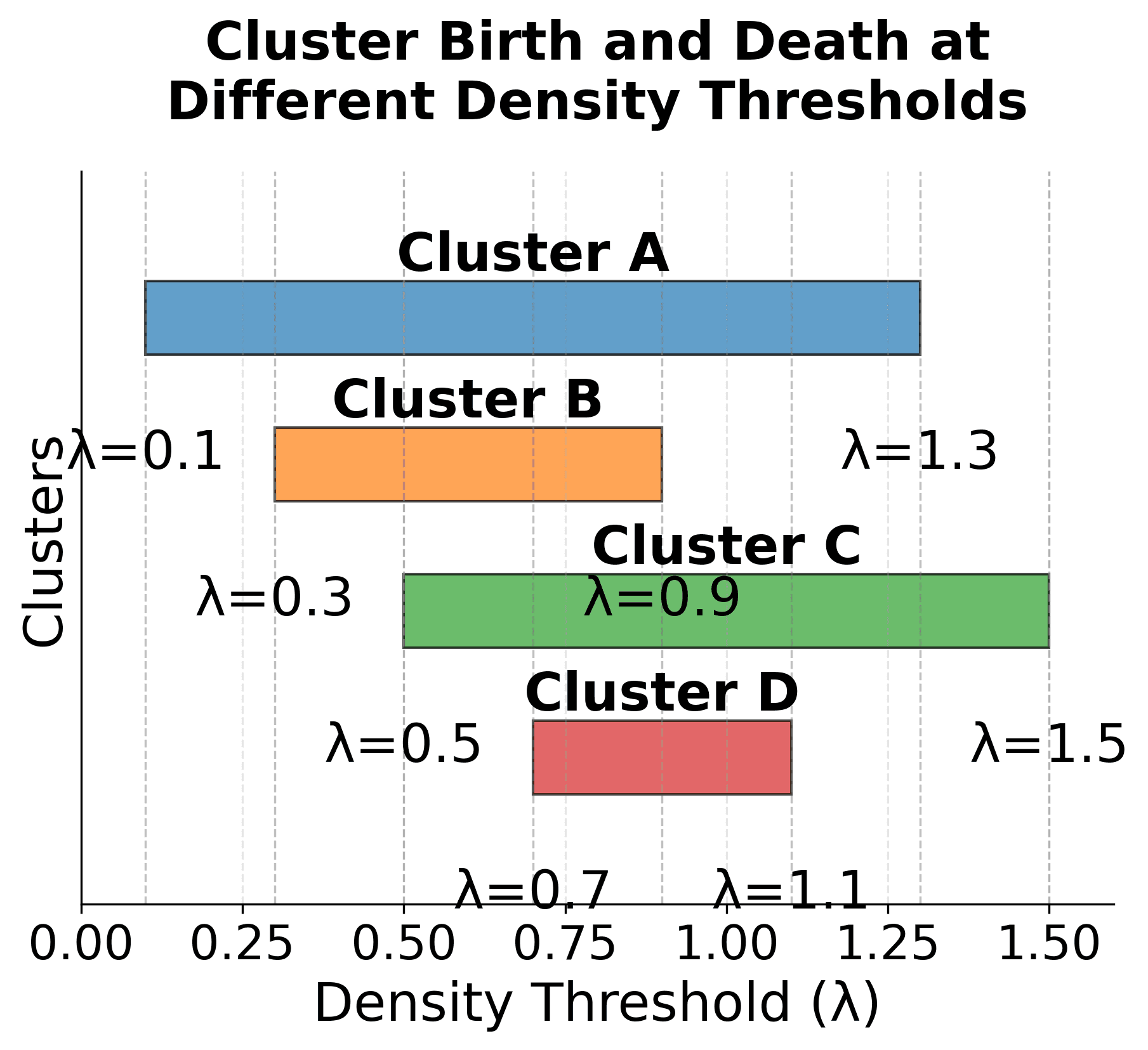
1. Cluster Lifespan: Each cluster is born at a specific density threshold (λ_birth) and dies at another threshold (λ_death). The width of each bar represents how long the cluster persists across different density levels.

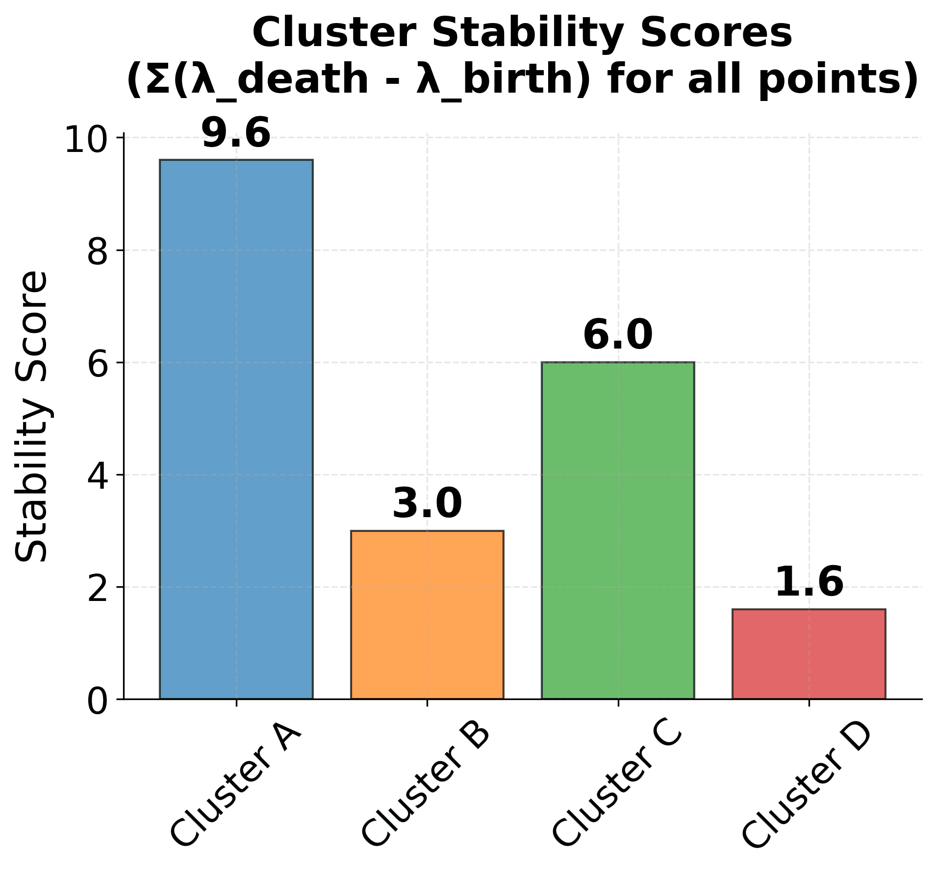
2. Stability Calculation: The stability score for each cluster is proportional to both the number of points in the cluster and how long it persists across density thresholds. Clusters that are both large and persistent receive higher stability scores.

3. Cluster Selection: The algorithm selects clusters with the highest stability scores, as these represent the most robust and meaningful structures in the data. In this example, Cluster A would be selected due to its high stability score.

Visualizing HDBSCAN

Let's create visualizations that demonstrate how HDBSCAN works and how it differs from other clustering methods.

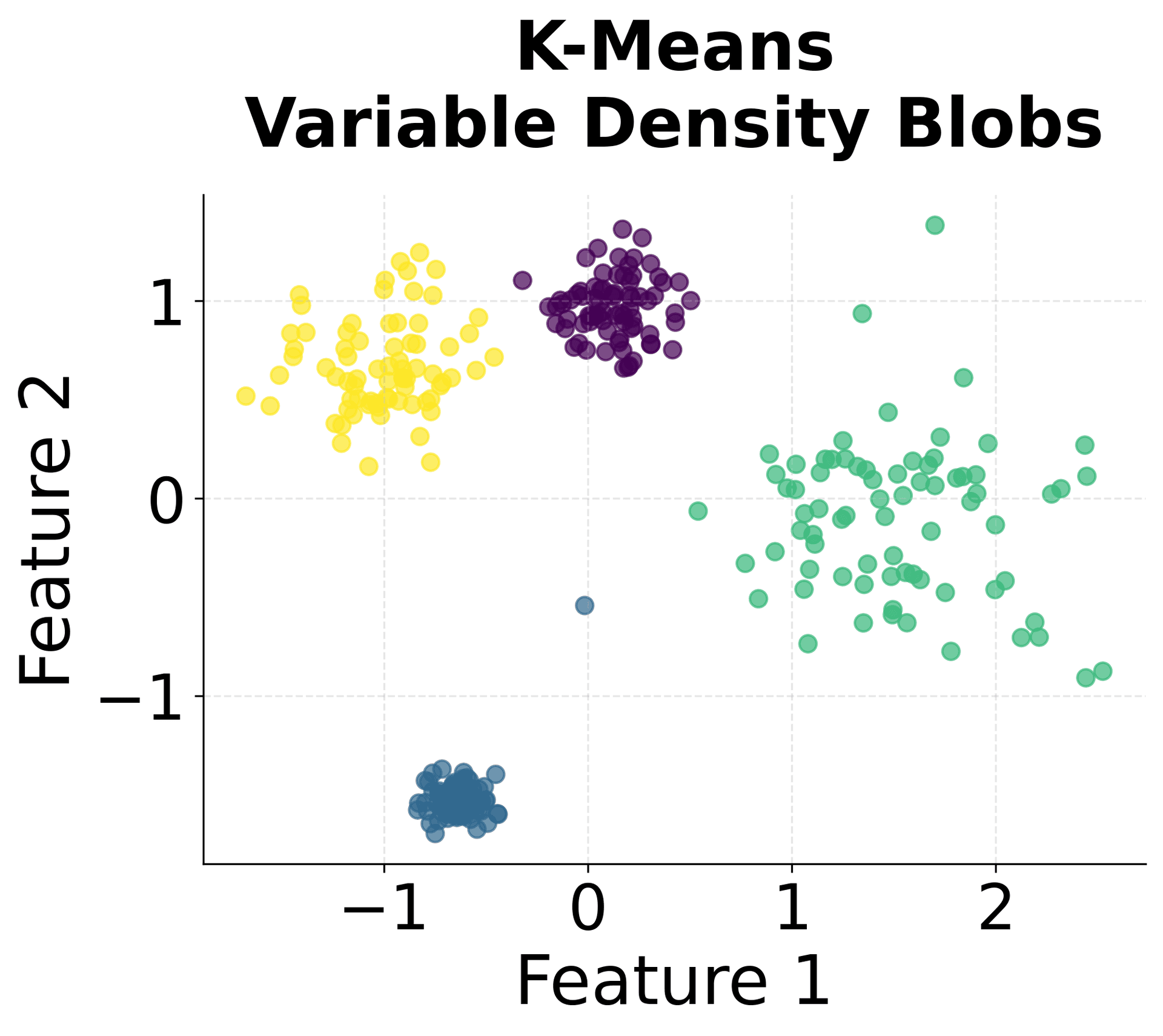
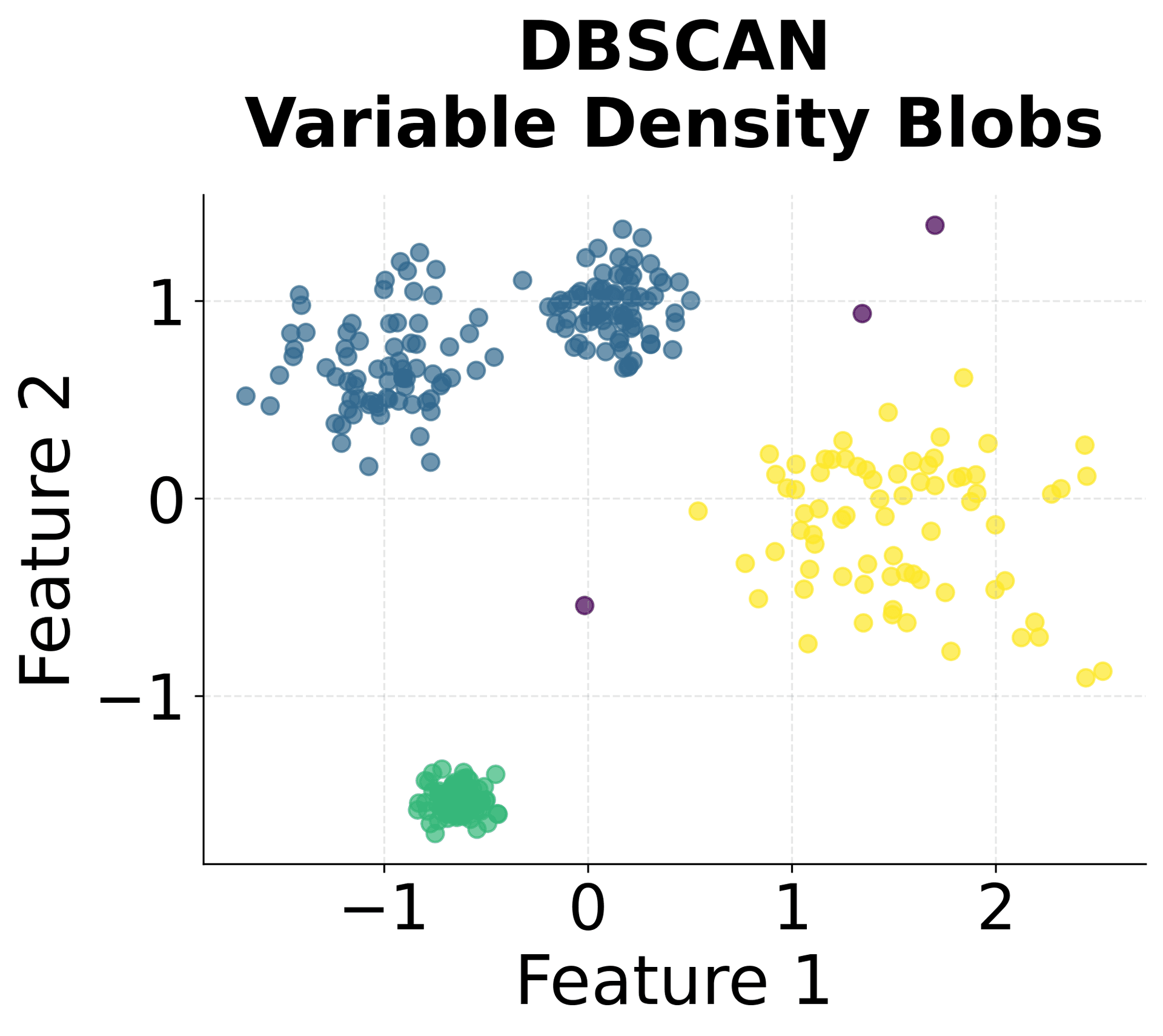
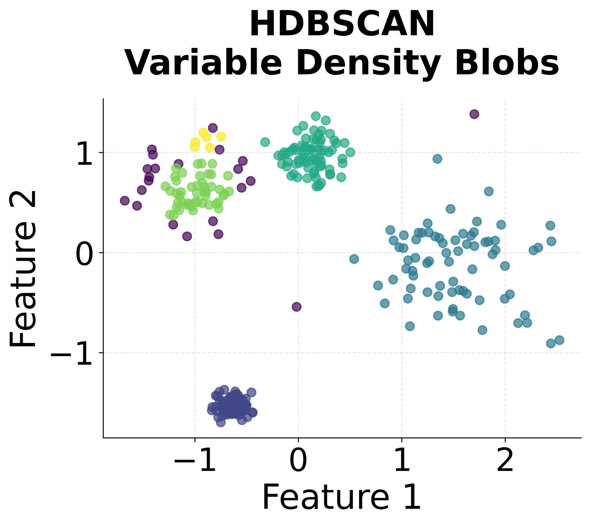
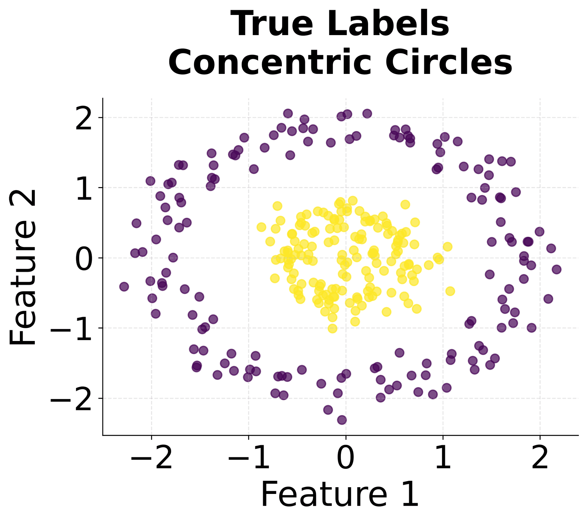
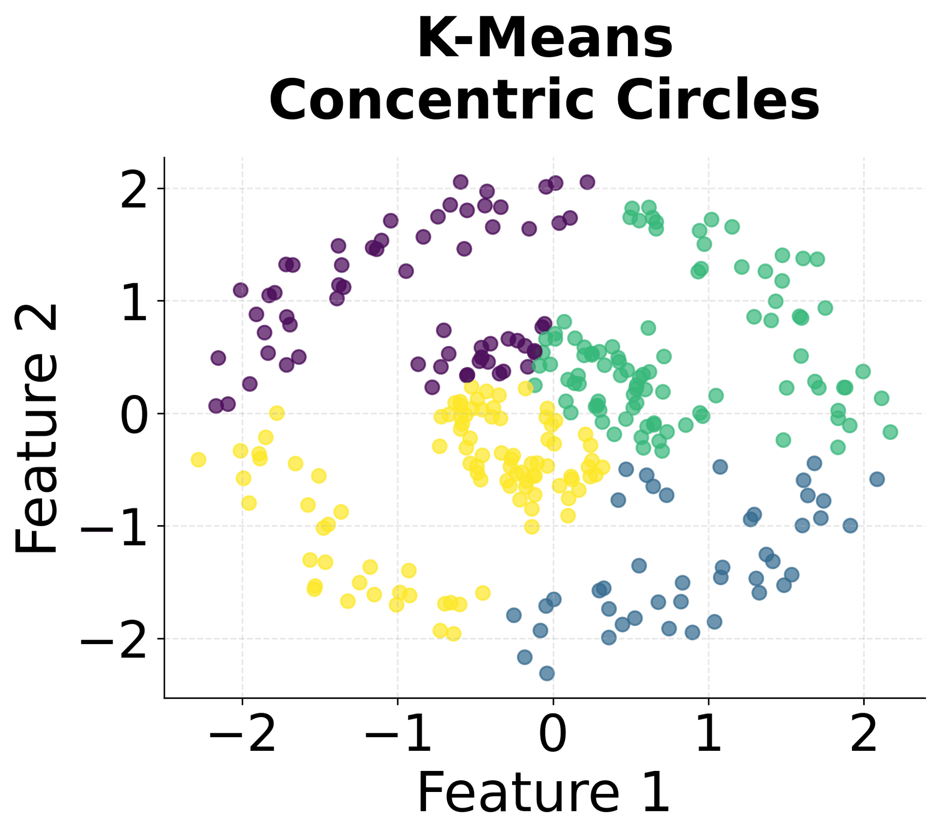
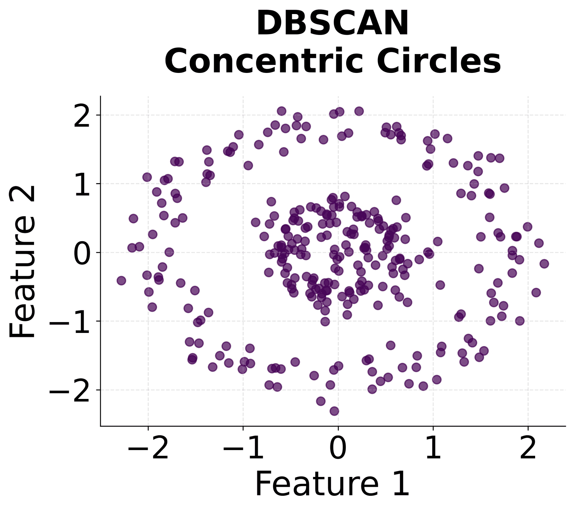
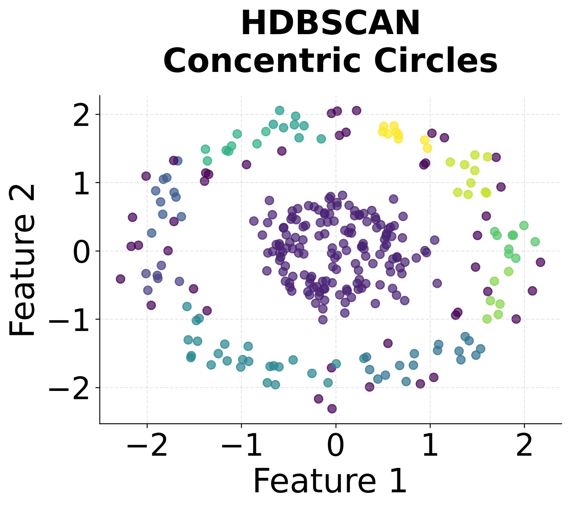
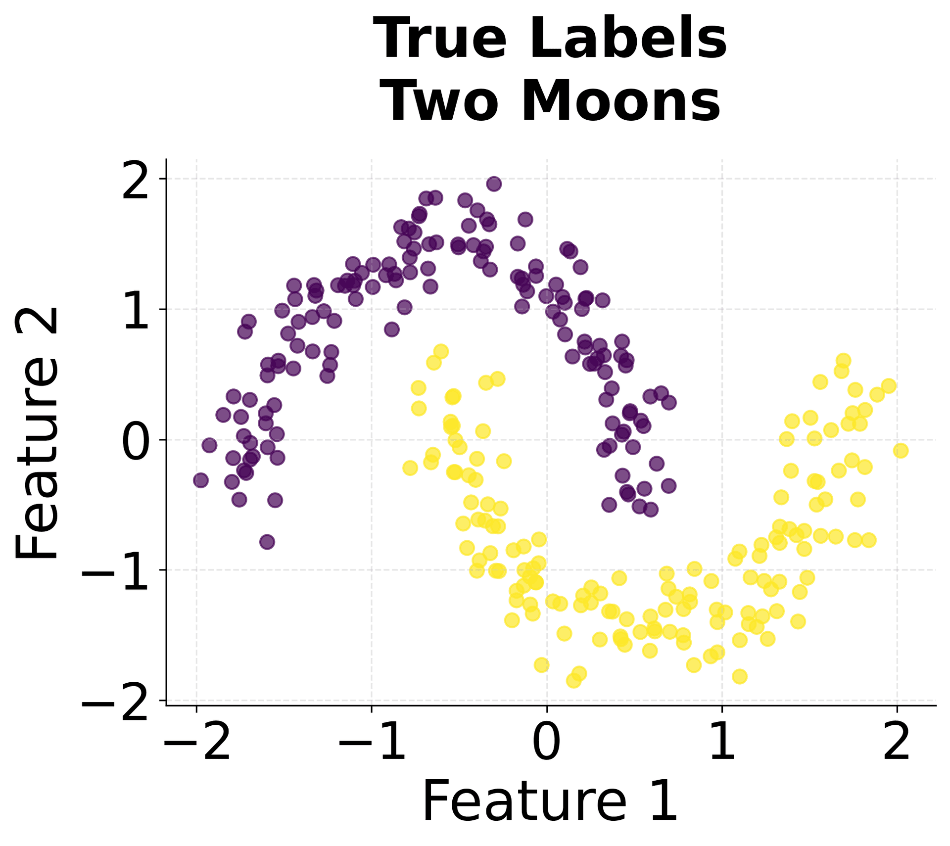
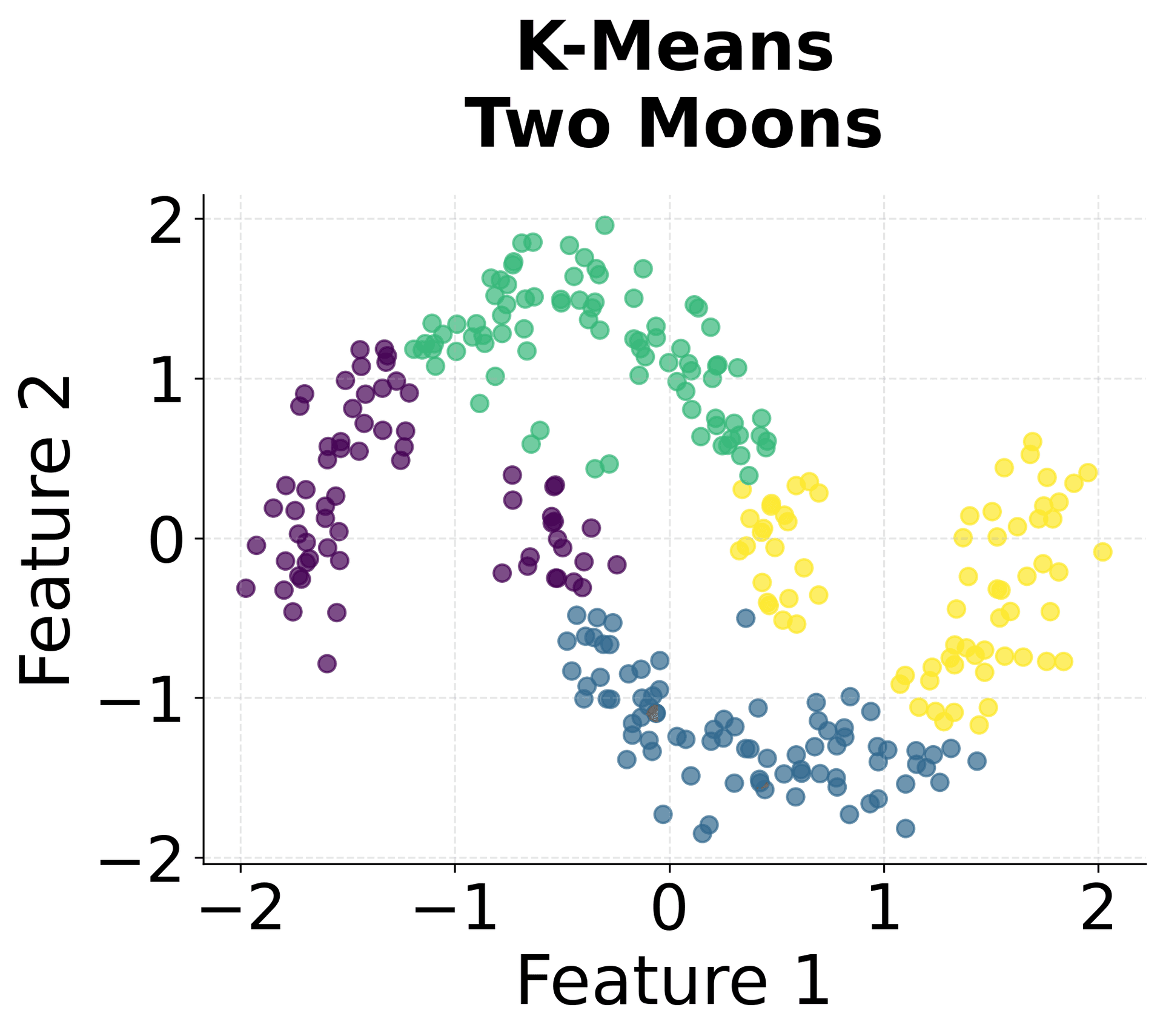
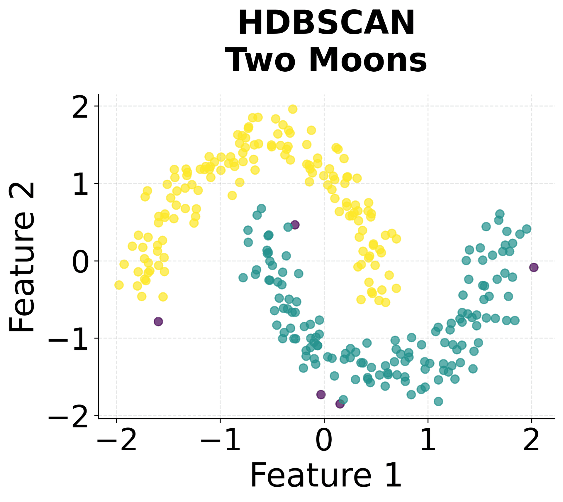
Here's how HDBSCAN performs compared to K-Means and DBSCAN across different types of data structures. You can see that HDBSCAN successfully handles variable density clusters, non-spherical shapes, and automatically determines the appropriate number of clusters.

Example

Let's work through a concrete example to understand how HDBSCAN processes data step by step. We'll use a simple 2D dataset and trace through the key calculations.

Now let's calculate the core distances and mutual reachability distances step by step:

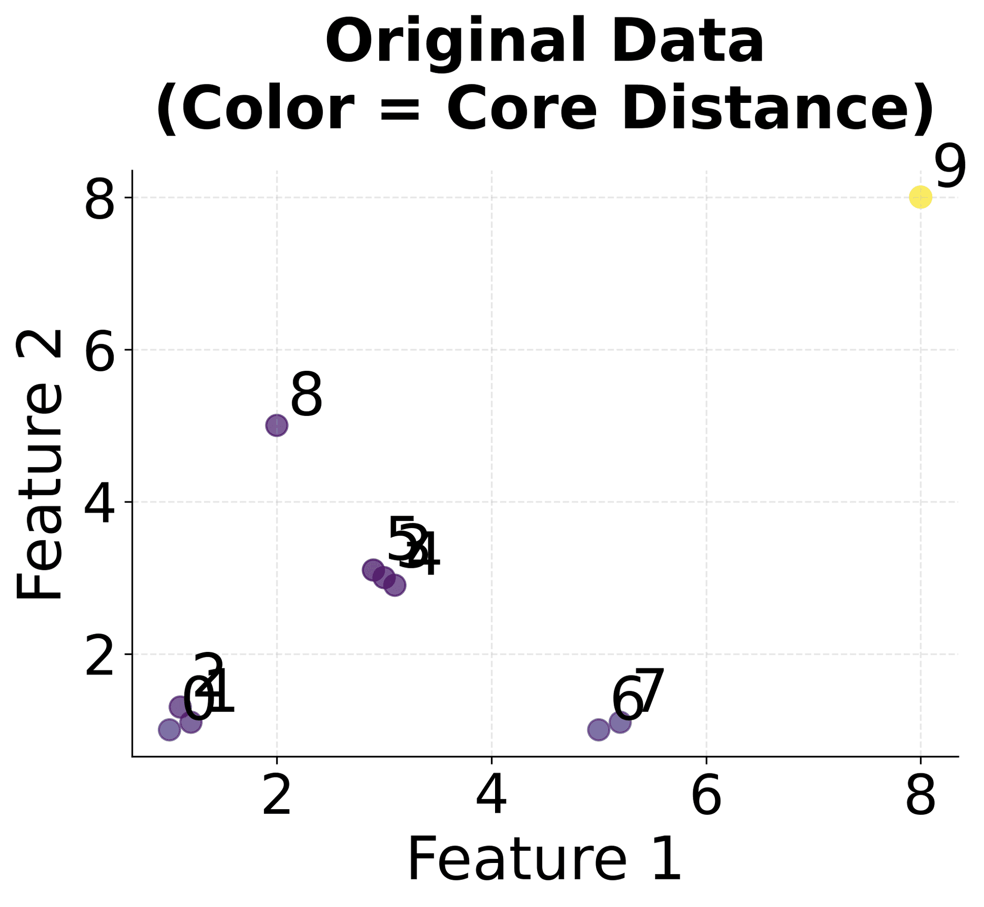
This example demonstrates the key steps of HDBSCAN:

1. Core Distance Calculation: Each point's core distance represents the distance to its k-th nearest neighbor, providing a local density measure.

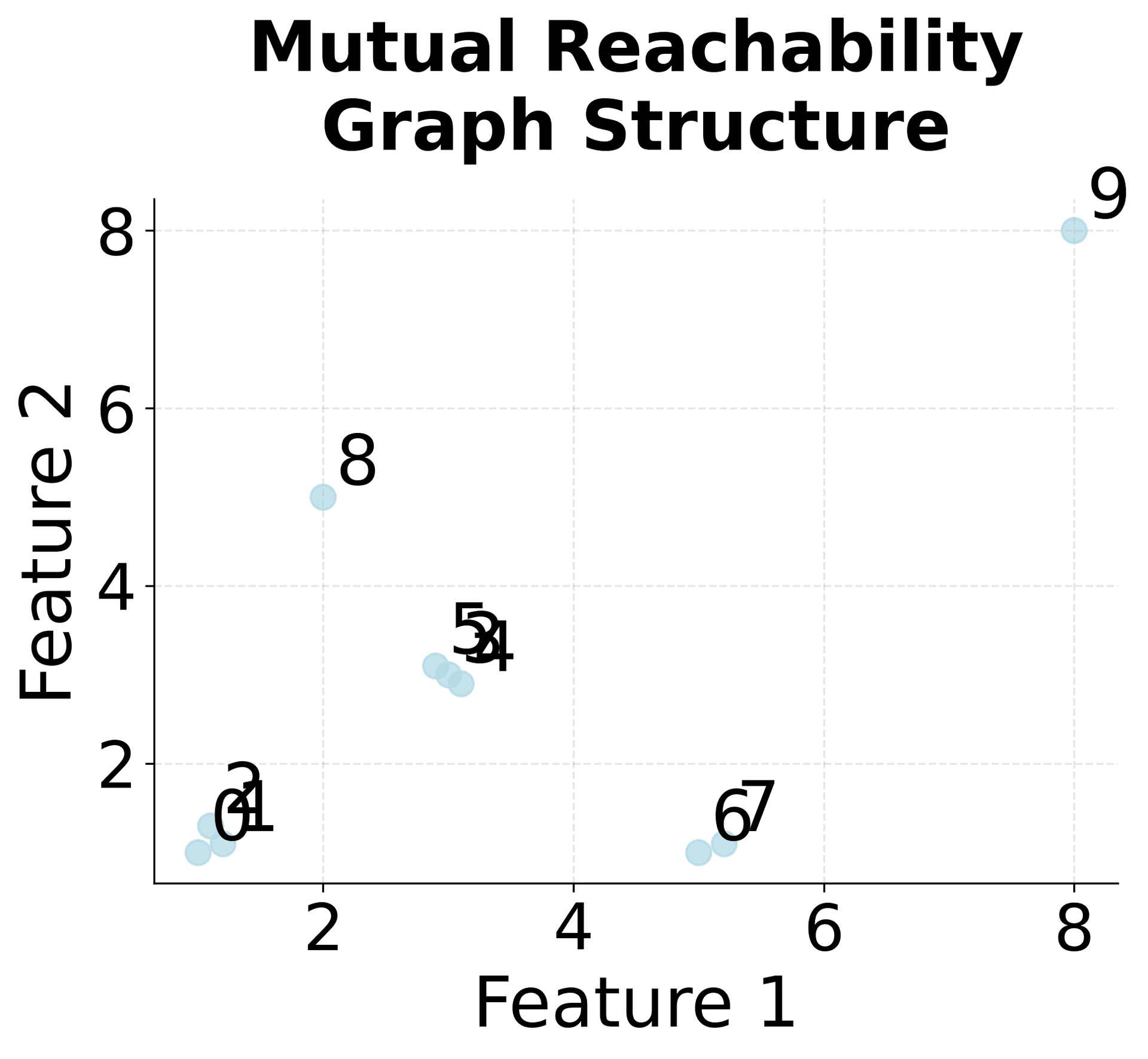
2. Mutual Reachability Distance: This distance metric ensures that points in dense regions are closer to each other, while points in sparse regions are farther apart, creating a more robust clustering foundation.

3. Minimum Spanning Tree: The MST connects all points with minimum total weight, creating a hierarchical structure that preserves the essential connectivity information.

The algorithm then uses this hierarchy to identify stable clusters by analyzing how clusters persist across different density thresholds.

Implementation

Let's work through a practical implementation of HDBSCAN using the hdbscan library, which provides a scikit-learn compatible interface. We'll start by creating a complex dataset and then apply HDBSCAN step by step.

Data Preparation

First, we'll generate a synthetic dataset with multiple clusters of varying densities and add some noise points to simulate real-world data:

The dataset now contains multiple clusters with different densities and noise points. Standardization is important because HDBSCAN relies on distance calculations.

Applying HDBSCAN

Now we'll apply HDBSCAN with appropriate parameters:

The min_cluster_size=10 parameter requires that clusters contain at least 10 points, while min_samples=5 controls the local density requirement for core points.

Evaluating Results

Let's calculate key metrics to evaluate the clustering performance:

Now let's display the evaluation results:

HDBSCAN identified five clusters, matching the true number of clusters in the dataset. The algorithm correctly labeled the noise points we added, demonstrating its ability to distinguish between meaningful clusters and outliers. The Adjusted Rand Score indicates strong agreement between the predicted clusters and the true labels, with values closer to 1.0 representing better agreement. This suggests the algorithm accurately recovered the underlying cluster structure despite the varying densities. The Silhouette Score suggests reasonably well-separated clusters, though the presence of noise points and variable cluster densities can affect this metric. A silhouette score above 0.5 generally indicates good cluster separation.

Visualizing the Results

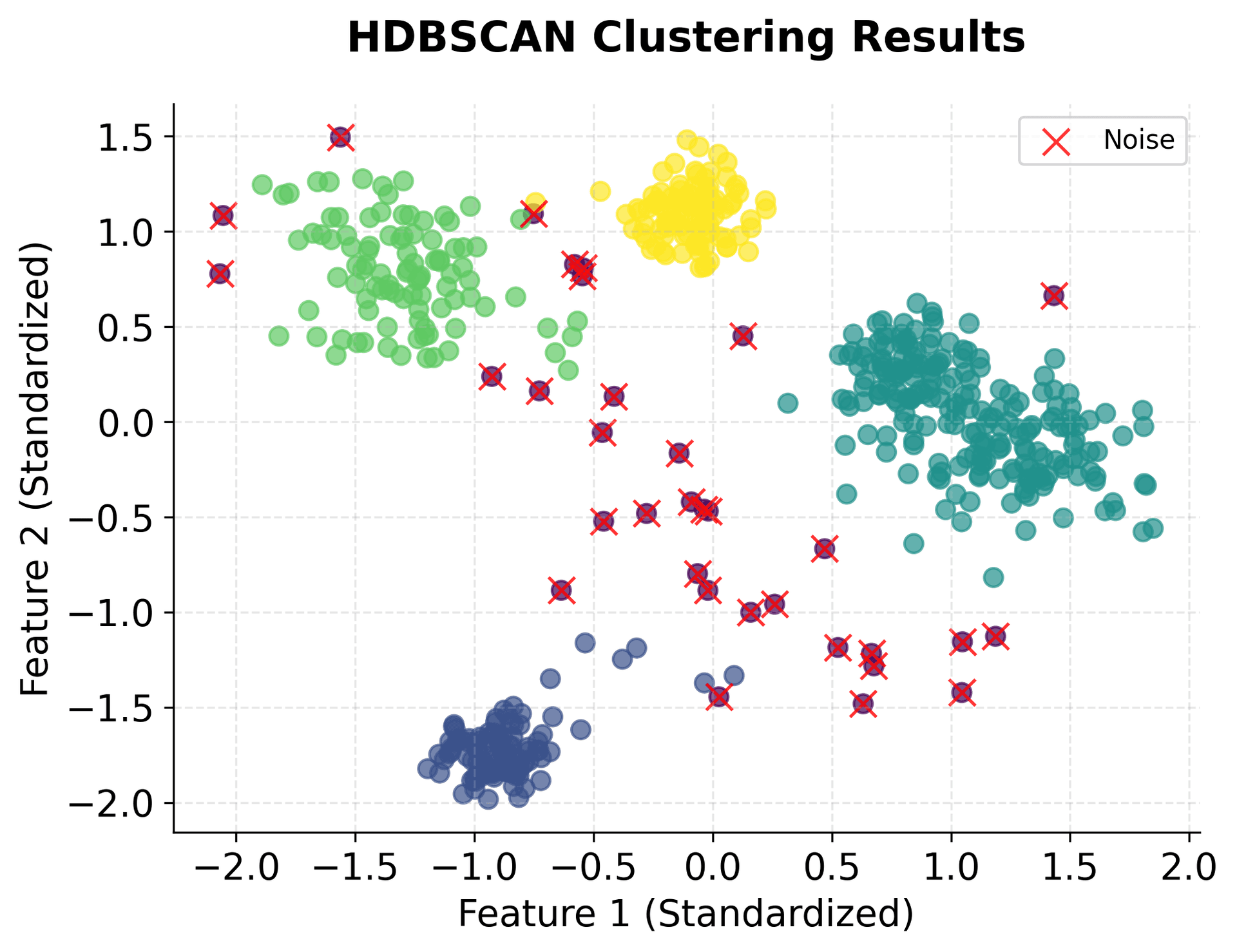
You can clearly see that HDBSCAN successfully identified all five clusters despite their varying densities and shapes, while correctly identifying noise points scattered throughout the space.

Parameter Sensitivity Analysis

Let's explore how different parameter settings affect the clustering results:

The results demonstrate how parameter selection affects clustering outcomes. Smaller min_cluster_size values (e.g., 5) tend to create more clusters and identify fewer noise points, which can fragment the data into many small groups. Larger values (e.g., 20) create fewer, more robust clusters but may merge distinct groups or miss smaller meaningful clusters. The optimal balance appears to be around min_cluster_size=10 and min_samples=5, which achieves the highest ARI score while maintaining reasonable cluster sizes. This parameter combination successfully identifies all five true clusters while correctly labeling noise points, demonstrating the importance of careful parameter tuning for optimal performance.

Key Parameters

Below are some of the main parameters that affect how HDBSCAN works and performs.

• min_cluster_size: Minimum number of points required to form a cluster (default: 5). Smaller values create more clusters but may include noise. Larger values create fewer, more robust clusters. A good starting point is 1-2% of your dataset size. For example, with 1000 points, start with min_cluster_size=10 to min_cluster_size=20.

• min_samples: Number of samples in a neighborhood for a point to be considered a core point (default: None, uses min_cluster_size). Controls the local density requirement. Should typically be set to about half of min_cluster_size. For example, if min_cluster_size=10, use min_samples=5.

• cluster_selection_epsilon: Distance threshold for cluster selection (default: 0.0). Points within this distance are considered for cluster membership. Lower values create more conservative clustering. Typically left at 0.0 unless you need to merge nearby clusters.

• metric: Distance metric to use for distance calculations (default: 'euclidean'). Options include 'euclidean', 'manhattan', 'cosine', etc. Euclidean works well for most numerical data, while cosine is useful for high-dimensional or text data.

• alpha: Distance scaling parameter for cluster selection (default: 1.0). Higher values create more conservative clustering. Typically left at 1.0 unless you need to adjust cluster selection behavior.

Key Methods

The following are the most commonly used methods for interacting with HDBSCAN.

• fit(X): Fits the HDBSCAN model to the data X. Computes the cluster hierarchy and identifies optimal clusters.

• fit_predict(X): Fits the model and returns cluster labels for each point. Returns -1 for noise points.

• predict(X): Predicts cluster labels for new data points using the fitted model. Note: HDBSCAN is primarily designed for clustering, not prediction.

• condensed_tree_: Returns the condensed tree structure showing cluster hierarchy and stability.

• cluster_persistence_: Returns the persistence (stability) scores for each cluster.

• outlier_scores_: Returns outlier scores for each point, with higher scores indicating more likely outliers.

Practical Applications

HDBSCAN is particularly valuable in several practical scenarios where traditional clustering methods fall short. In customer segmentation, HDBSCAN excels because customer groups often have varying densities and complex shapes that don't conform to spherical clusters. The algorithm can automatically identify the optimal number of customer segments while handling outliers (such as high-value customers who don't fit standard patterns) as noise points.

The algorithm is also highly effective in anomaly detection applications, where the goal is to identify normal patterns and flag unusual observations. Since HDBSCAN explicitly identifies noise points, it provides a natural framework for anomaly detection without requiring separate algorithms. This makes it particularly useful in fraud detection, network security, and quality control applications.

In bioinformatics and genomics, HDBSCAN's ability to handle clusters of varying densities is important when analyzing gene expression data or protein structures. Biological data often contains clusters with different characteristics, and the hierarchical approach allows researchers to explore nested structures and relationships that might be missed by other methods.

Best Practices

To achieve the best results with HDBSCAN, choose appropriate values for min_cluster_size and min_samples based on your data characteristics and clustering goals. A good starting point for min_cluster_size is often 1-2% of your total dataset size, and min_samples should typically be set to about half of min_cluster_size. This balance helps identify meaningful clusters while filtering out noise. For example, with a dataset of 1000 points, start with min_cluster_size=10 to min_cluster_size=20 and min_samples=5 to min_samples=10. Adjust these values based on your domain knowledge: if you expect larger, more cohesive clusters, increase min_cluster_size; if you want to capture smaller but meaningful groups, decrease it.

When evaluating your clustering results, use multiple metrics such as silhouette analysis and domain knowledge to validate the clustering quality. The proportion of noise points can also provide insights: if too many points are labeled as noise (e.g., more than 30-40% of your data), consider reducing min_cluster_size or min_samples. Conversely, if too few points are labeled as noise (e.g., less than 5%), these parameters may be too small and you may be overfitting to noise. Set the random_state parameter for reproducibility when using approximate methods or sampling strategies. For datasets with known cluster structures, compare HDBSCAN's automatic cluster count with your domain knowledge to validate the results.

Data Requirements and Preprocessing

HDBSCAN requires numerical data with features that are comparable in scale. Since the algorithm uses distance calculations, features with larger scales will dominate the clustering process, potentially leading to misleading results. Apply StandardScaler or MinMaxScaler before clustering to ensure all features contribute equally to the distance calculations. StandardScaler is typically preferred as it centers the data around zero and scales to unit variance, making the distance metric more interpretable.

The algorithm works best with clean, complete datasets that have minimal missing values. Missing values should be imputed using appropriate strategies (such as mean imputation for numerical features or mode imputation for categorical features) before clustering. Categorical variables need to be encoded before clustering. One-hot encoding works well for nominal variables, while label encoding may be appropriate for ordinal variables. The choice of encoding method can impact results, so consider the nature of your categorical variables when making this decision.

Additionally, ensure your dataset has sufficient data points relative to the number of features to avoid the curse of dimensionality, which can lead to poor clustering performance in high-dimensional spaces. As a rule of thumb, aim for at least 10-20 times more data points than features. For high-dimensional data (typically more than 50-100 features), consider dimensionality reduction techniques such as PCA before applying HDBSCAN to improve both computational efficiency and clustering quality.

Common Pitfalls

One frequent mistake is choosing inappropriate values for min_cluster_size and min_samples, which can result in either too many small clusters or too few large clusters. Values that are too small may fragment the data into many small clusters and misclassify noise as clusters, while values that are too large may merge distinct clusters or miss smaller but meaningful groups. To avoid this, start with the 1-2% guideline for min_cluster_size and systematically adjust based on your results, using domain knowledge to guide your choices.

Another significant pitfall is over-interpreting the clustering results, as HDBSCAN typically produces clusters even when no meaningful structure exists in the data. Validate clustering results using multiple evaluation methods and domain knowledge to ensure the clusters make sense from a practical perspective. Failing to standardize data before clustering is also a common error that can lead to misleading results, as features with larger scales will dominate the distance calculations. Additionally, applying HDBSCAN directly to high-dimensional data without dimensionality reduction can result in poor performance due to the curse of dimensionality, where distance metrics become less meaningful as the number of dimensions increases.

Computational Considerations

HDBSCAN's computational complexity is primarily determined by the mutual reachability distance calculation and MST construction, which scale as $O(n^2)$ in the worst case. For large datasets (typically >10,000 points), you may need to consider sampling strategies or use approximate methods to make the algorithm computationally feasible. The algorithm's memory requirements can also be substantial for large datasets due to the need to store the full distance matrix, which requires $O(n^2)$ memory space.

For very large datasets, consider using HDBSCAN on a representative sample of the data (e.g., 5,000-10,000 points) selected through stratified sampling if you have class labels, or random sampling otherwise. Alternatively, use approximate HDBSCAN methods that trade some accuracy for improved computational efficiency, which may be suitable for large-scale applications. Some implementations offer approximate nearest neighbor methods that can reduce the computational burden. For datasets with more than 50,000 points, consider using alternative scalable clustering methods such as Mini-Batch K-means for initial exploration, or apply HDBSCAN to data subsets and combine the results.

Performance and Deployment Considerations

Evaluating HDBSCAN performance requires careful consideration of both the clustering quality and the noise detection capabilities. Use metrics such as silhouette analysis to evaluate cluster quality, and consider the proportion of noise points as an indicator of the algorithm's effectiveness. A silhouette score above 0.5 generally indicates reasonable cluster separation, while scores below 0.3 suggest poor clustering quality. The proportion of noise points should align with your domain expectations: if you expect 5-10% outliers, but HDBSCAN identifies 40% as noise, this may indicate parameter misconfiguration or that the data lacks clear cluster structure.

The algorithm is well-suited for applications where noise detection is important and when clusters may have irregular shapes or varying densities. In production, consider using HDBSCAN for initial data exploration and then applying more scalable methods for large-scale clustering tasks. The parameter sensitivity of HDBSCAN requires careful tuning for optimal performance, so plan for experimentation and validation when deploying the algorithm in production environments. When deploying in production, monitor the proportion of noise points and cluster stability over time, as changes in data distribution may require parameter adjustments. For real-time applications, the $O(n^2)$ complexity makes HDBSCAN less suitable; instead, use it for batch processing or offline analysis where computational time is less critical.

Summary

HDBSCAN combines the density-based approach of DBSCAN with hierarchical clustering principles. The algorithm automatically determines the number of clusters while handling noise and clusters of varying densities, making it valuable for real-world applications where data characteristics are unknown or complex.

HDBSCAN's mathematical foundation, based on mutual reachability distances and cluster stability measures, provides a principled approach to cluster selection that addresses many limitations of traditional clustering methods. The hierarchical structure allows analysis of nested clusters and provides insights into the data structure that other algorithms might miss.

While HDBSCAN has computational limitations and parameter sensitivity challenges, its strengths in handling complex, real-world data make it a useful tool in the data scientist's toolkit. The algorithm's robustness to noise, ability to identify clusters of arbitrary shapes, and automatic cluster selection capabilities make it valuable for exploratory data analysis and applications where traditional clustering assumptions don't hold.

Quiz

Ready to test your understanding? Take this quick quiz to reinforce what you've learned about HDBSCAN clustering.