InteractiveK-means Clustering: Complete Guide with Algorithm, Implementation & Best Practices

K-means Clustering

K-means clustering is one of the fundamental and widely-used unsupervised learning algorithms in machine learning. The algorithm partitions a dataset into k distinct, non-overlapping clusters, where each data point belongs to the cluster with the nearest mean (centroid). The "k" in K-means refers to the number of clusters we want to identify, which needs to be specified before running the algorithm.

The algorithm works by iteratively assigning data points to clusters and updating cluster centroids until convergence. It's particularly effective for datasets where clusters are roughly spherical and well-separated. K-means is often used as a baseline method for clustering problems and serves as a stepping stone to more sophisticated clustering techniques.

Unlike supervised learning methods that require labeled training data, K-means operates entirely on unlabeled data, making it valuable for exploratory data analysis, customer segmentation, image compression, and pattern recognition. The algorithm assumes that clusters are convex and isotropic, meaning they have roughly equal variance in all directions.

K-means clustering differs from hierarchical clustering in that it requires us to specify the number of clusters beforehand, and it produces a flat clustering structure rather than a tree-like hierarchy. It also differs from density-based clustering methods like DBSCAN, which can find clusters of arbitrary shapes and automatically determine the number of clusters.

Advantages

K-means clustering offers several advantages that make it a popular choice for many clustering applications. First, the algorithm is computationally efficient and scales well to large datasets, with a time complexity of O(nkt), where n is the number of data points, k is the number of clusters, and t is the number of iterations. This makes it practical for real-world applications with millions of data points.

The algorithm is conceptually simple and easy to understand, making it accessible to practitioners with varying levels of mathematical background. The iterative nature of the algorithm is intuitive: we start with random centroids, assign points to the nearest centroid, update the centroids, and repeat until convergence. This simplicity also makes the algorithm easy to implement and debug.

K-means produces compact, well-defined clusters when the underlying data structure matches its assumptions. The algorithm works particularly well when clusters are roughly spherical and have similar sizes, which is common in many real-world applications. Additionally, the resulting centroids provide interpretable representatives for each cluster, which can be valuable for understanding the characteristics of different groups in the data.

Disadvantages

Despite its popularity, K-means clustering has several limitations that practitioners should be aware of. The most significant limitation is that the algorithm requires us to specify the number of clusters k beforehand, which is often unknown in practice. Choosing the wrong value of k can lead to poor clustering results, and determining the optimal k typically requires additional analysis techniques like the elbow method or silhouette analysis.

The algorithm assumes that clusters are spherical and have roughly equal variance, which may not hold for many real-world datasets. K-means struggles with clusters that are elongated, have different sizes, or have non-spherical shapes. This limitation can lead to incorrect cluster assignments when the underlying data structure doesn't match these assumptions.

K-means is sensitive to the initialization of cluster centroids and can converge to local optima rather than the global optimum. Different random initializations can produce different clustering results, making the algorithm somewhat unstable. While techniques like k-means++ initialization help mitigate this issue, the problem of local optima remains a fundamental challenge.

The algorithm is also sensitive to outliers, which can affect the position of cluster centroids and the overall clustering quality. Outliers can pull centroids away from the true cluster centers, leading to distorted cluster boundaries and poor performance on the majority of the data.

Formula

K-means clustering is fundamentally about finding natural groupings in data by minimizing how spread out points are within each cluster. To understand the mathematics behind this intuitive goal, we'll build up from a simple question to the complete algorithm, revealing why each mathematical component is necessary and how they work together to solve the clustering problem.

The Core Question: What Makes a Good Clustering?

Imagine you have a collection of data points scattered across space, and you want to organize them into k groups. What would make one grouping better than another? Intuitively, we want points within the same group to be close together, tightly packed around some central location. This intuition leads us to the mathematical foundation of K-means.

For each cluster, we can represent its "center" by a single point called the centroid. Think of the centroid as the average position of all points in that cluster: it's the natural meeting point that minimizes the total distance to all cluster members. Once we have centroids, we can measure how "tight" each cluster is by calculating how far each point is from its centroid. The smaller these distances, the more compact and well-defined our clusters are.

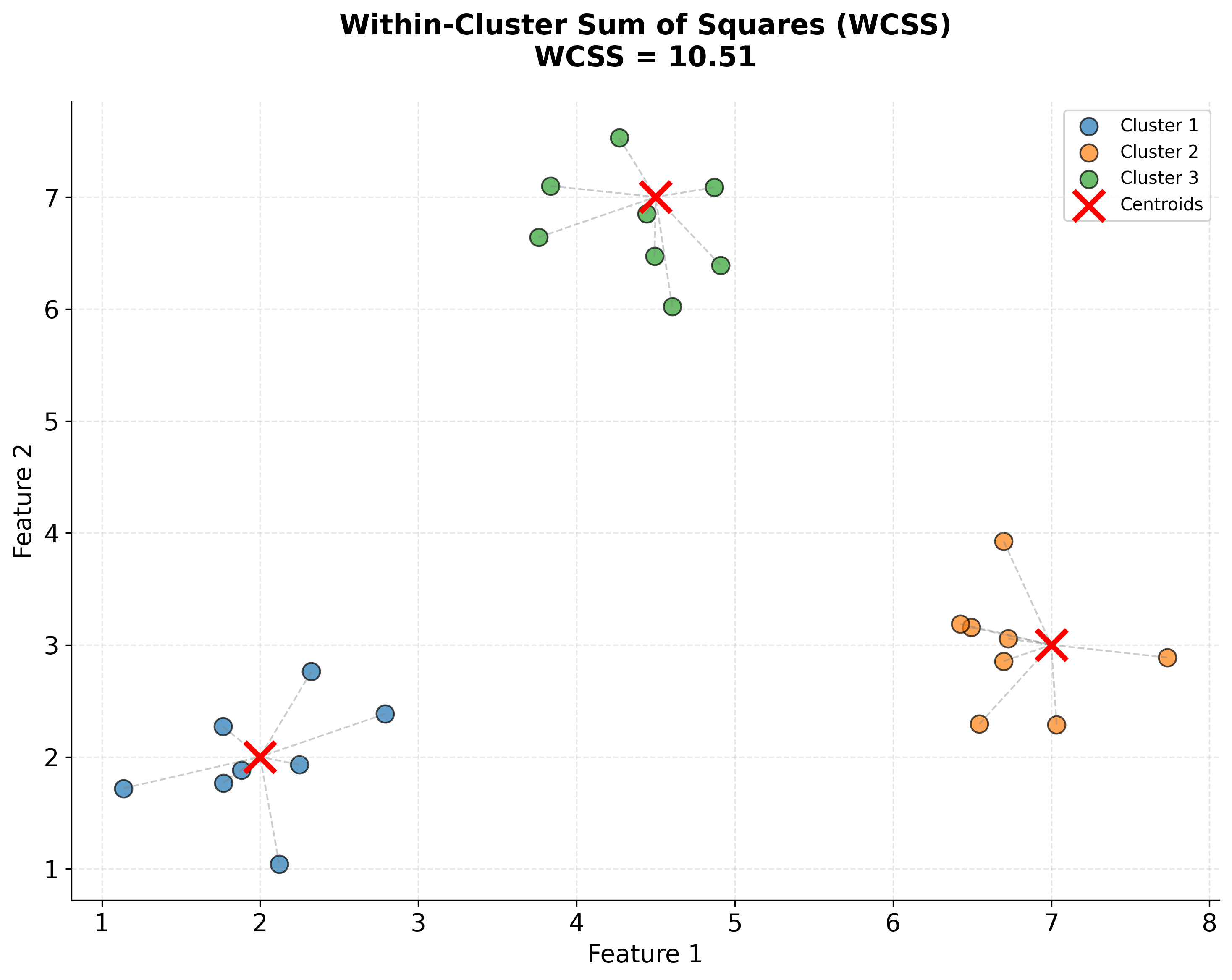
This brings us to the fundamental objective: we want to find cluster assignments and centroid positions that minimize the total squared distance from each point to its assigned centroid. This is called the within-cluster sum of squares (WCSS) or inertia, and it's what K-means tries to minimize.

Building the Objective Function

Let's formalize this intuition step by step. Suppose we want to partition our dataset into k clusters, which we'll call $C_1, C_2, \ldots, C_k$. Each cluster $C_i$ is simply a set of data points that belong together. For each cluster, we'll compute a centroid $\mu_i$ that represents the cluster's center.

Now, how do we measure the quality of this clustering? We calculate the squared distance from each point to its cluster's centroid, then sum up all these squared distances across all clusters:

Let's unpack what each part means:

• $C_1, C_2, \ldots, C_k$: The k clusters we're trying to find. Each cluster is a set of data points.
• $x \in C_i$: "For each data point x that belongs to cluster i." This notation tells us to consider every point in the cluster.
• $\mu_i$: The centroid (mean position) of cluster i. This is the point that represents the cluster's center.
• $\|x - \mu_i\|^2$: The squared Euclidean distance between point x and its cluster's centroid $\mu_i$. This measures how far the point is from its cluster center.
• The double summation: The inner sum ($\sum_{x \in C_i}$) adds up distances for all points in cluster i. The outer sum ($\sum_{i=1}^{k}$) adds up the results across all k clusters.

Our goal is to find the cluster assignments and centroids that minimize this total squared distance:

Why squared distances? You might wonder why we square the distances rather than just using regular distances. There are two important reasons:

1. Mathematical tractability: Squared distances make the optimization problem differentiable and easier to solve mathematically. The square function is smooth everywhere, which allows us to use calculus-based optimization techniques.

2. Emphasis on outliers: Squaring distances penalizes points that are far from their centroids more heavily than points that are close. A point that's twice as far away contributes four times as much to the objective function. This encourages the algorithm to create tight, compact clusters.

Let's visualize what the WCSS objective function actually represents:

Understanding Distance in Detail

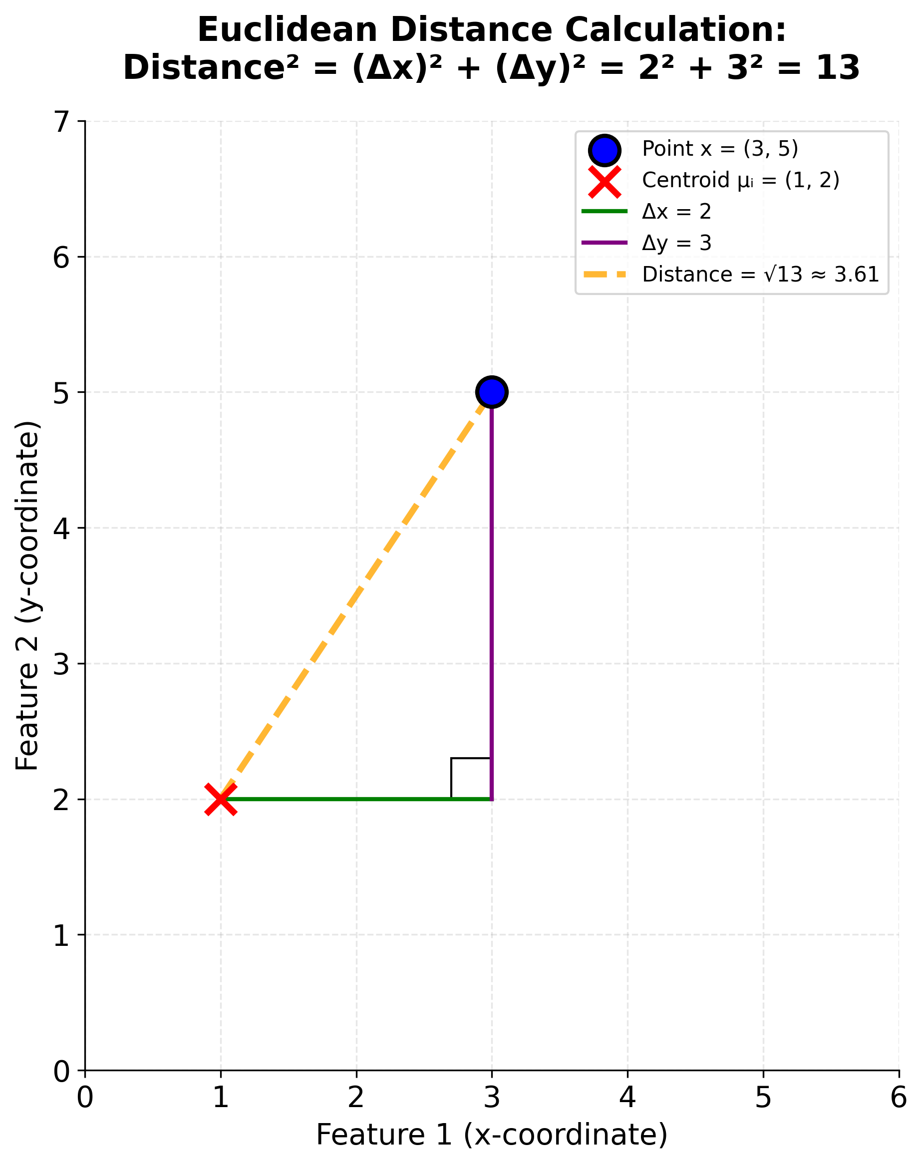
Let's zoom in on the distance calculation itself. When we write $\|x - \mu_i\|^2$, we're computing the squared Euclidean distance between two points in d-dimensional space. If our data has d features, then each point x and each centroid $\mu_i$ is a d-dimensional vector.

The squared Euclidean distance is calculated by summing the squared differences across all dimensions:

Here's what each component means:

• $d$: The number of features (dimensions) in our data. For example, if we're clustering customers based on age, income, and purchase frequency, then d = 3.
• $x_j$: The value of the j-th feature for data point x. For instance, $x_2$ might be the income of a customer.
• $\mu_{i,j}$: The value of the j-th feature for centroid $\mu_i$. This is the average value of feature j across all points in cluster i.
• $(x_j - \mu_{i,j})^2$: The squared difference between the point's feature value and the centroid's feature value for dimension j.

For example, if we have a 2D point $x = (3, 5)$ and a centroid $\mu_i = (1, 2)$, the squared distance is:

Let's visualize this distance calculation geometrically:

This distance calculation treats all dimensions equally, which is why data standardization is crucial before applying K-means. If one feature has values in the thousands while another has values between 0 and 1, the larger-scale feature will dominate the distance calculation and disproportionately influence the clustering.

Computing the Centroid: The Natural Center

Now that we understand how to measure distances, let's see how to compute the centroid of a cluster. The centroid is simply the mean (average) position of all points in the cluster. This choice isn't arbitrary: the mean is mathematically special because it's the point that minimizes the sum of squared distances to all other points in the set.

For cluster i, the centroid is calculated as:

Breaking this down:

• $|C_i|$: The number of points in cluster i. The vertical bars denote the cardinality (size) of the set.
• $\sum_{x \in C_i} x$: The sum of all data points in cluster i. Since each point is a vector, this is a vector sum.
• $\frac{1}{|C_i|}$: We divide by the number of points to get the average.

For example, if cluster 1 contains three 2D points: $(1,2)$, $(3,4)$, and $(5,6)$, the centroid is:

The centroid $(3, 4)$ is the average position of the three points: it's the natural "center of mass" of the cluster.

The K-means Algorithm: An Iterative Solution

We now have all the pieces we need, but there's a challenge: finding the optimal clusters and centroids simultaneously is computationally intractable for most datasets. The problem is NP-hard, meaning there's no known efficient algorithm to find the globally optimal solution.

K-means solves this by using an iterative approach that alternates between two steps:

1. Fix the centroids, optimize the cluster assignments: Given current centroid positions, assign each point to its nearest centroid.
2. Fix the cluster assignments, optimize the centroids: Given current cluster assignments, recompute centroids as the mean of their assigned points.

By alternating between these two steps, the algorithm is guaranteed to converge to a local minimum of the objective function. While this might not be the global optimum, it's often a good solution in practice, especially with smart initialization strategies like k-means++.

Let's formalize this iterative process:

Step 1: Initialization

Choose k initial centroids $\mu_1^{(0)}, \mu_2^{(0)}, \ldots, \mu_k^{(0)}$. The superscript $(0)$ indicates these are the centroids at iteration 0 (the starting point). The choice of initial centroids can significantly impact the final result, which is why k-means++ initialization is preferred over random selection.

Step 2: Assignment Step

For each data point $x$, assign it to the cluster whose centroid is closest. Mathematically, at iteration $t$, cluster $i$ contains all points for which centroid $\mu_i^{(t)}$ is the nearest:

Let's decode this notation:

• $C_i^{(t)}$: The set of points assigned to cluster i at iteration t.
• $x$: A data point we're considering.
• $\|x - \mu_i^{(t)}\|^2$: The squared distance from point x to centroid i.
• "$\leq \|x - \mu_j^{(t)}\|^2$ for all $j \neq i$": Point x is closer to centroid i than to any other centroid j.

In plain English: "Cluster i contains all points that are closer to centroid i than to any other centroid."

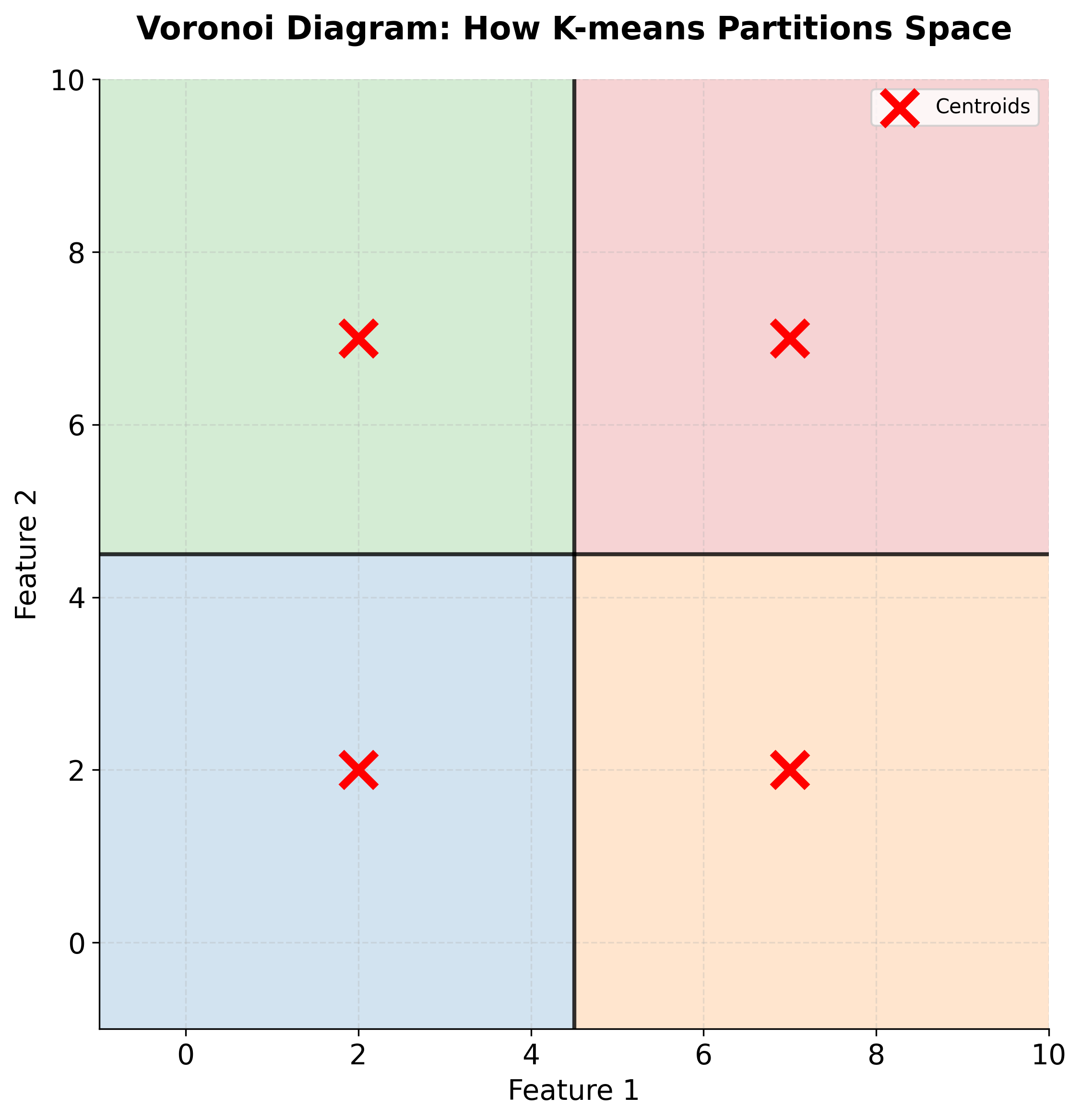
This assignment step creates a Voronoi diagram in the feature space: each cluster's region consists of all points closer to its centroid than to any other centroid. The boundaries between clusters are hyperplanes that bisect the lines connecting adjacent centroids.

Let's visualize what a Voronoi diagram looks like:

Step 3: Update Step

Once we've assigned all points to clusters, we recompute each centroid as the mean of its assigned points:

The superscript $(t+1)$ indicates this is the new centroid for the next iteration. This update moves each centroid to the center of its cluster, which will generally reduce the within-cluster sum of squares.

Step 4: Convergence Check

We repeat steps 2 and 3 until one of these conditions is met:

• The centroids no longer change (or change by less than a small threshold)
• The cluster assignments no longer change
• We reach a maximum number of iterations

The algorithm is guaranteed to converge because each step either decreases or maintains the objective function value (it can never increase). Eventually, we reach a point where no further improvement is possible, and the algorithm stops.

Compact Matrix Notation

For those familiar with linear algebra, we can express the K-means assignment step more compactly using matrix notation. Let X be our $n \times d$ data matrix (n points, d features) and M be our $k \times d$ centroid matrix (k centroids, d features).

For each point, the assignment step finds:

where $X_j$ is the j-th row of X (the j-th data point) and $M_i$ is the i-th row of M (the i-th centroid). This notation emphasizes that we're finding the centroid index i that minimizes the distance for each point.

Mathematical Properties and Guarantees

Understanding the mathematical properties of K-means helps us know what to expect and when to trust the results:

Convergence Guarantee

K-means is guaranteed to converge to a local minimum of the objective function. This is because:

1. The assignment step assigns each point to its nearest centroid, which can only decrease (or maintain) the total squared distance.
2. The update step moves each centroid to the mean of its cluster, which minimizes the sum of squared distances for that cluster.
3. Since both steps decrease or maintain the objective function, and there are only finitely many possible cluster assignments, the algorithm must eventually stop improving and converge.

However, this convergence is to a local minimum, not necessarily the global minimum. Different initializations can lead to different final clusterings, which is why running K-means multiple times with different random seeds (controlled by the n_init parameter) is recommended.

Computational Complexity

The algorithm has a time complexity of O(nkdt), where:

• n: Number of data points
• k: Number of clusters
• d: Number of features (dimensions)
• t: Number of iterations until convergence

In practice, t is typically much smaller than n (often less than 100 iterations), making K-means quite efficient even for large datasets. The algorithm scales linearly with the number of data points, which is excellent for big data applications.

Optimality of Centroids

The centroids produced by K-means are optimal in a specific sense: given a fixed cluster assignment, the centroids that minimize the within-cluster sum of squares are exactly the means of the clusters. This is a mathematical fact that follows from calculus: the derivative of the sum of squared distances with respect to the centroid position is zero at the mean.

This optimality property is what makes the update step so effective: by moving centroids to the mean of their clusters, we're guaranteed to improve (or at least not worsen) the objective function for that fixed assignment.

Space Partitioning

K-means creates a partition of the feature space into k regions, where each region contains all points closest to a particular centroid. These regions are convex polytopes (generalized polygons in higher dimensions) bounded by hyperplanes. This geometric structure explains why K-means works well for spherical, well-separated clusters but struggles with elongated or irregularly shaped clusters: the algorithm is fundamentally constrained to create convex regions.

Visualizing K-means Clustering

Let's create a comprehensive visualization that demonstrates how K-means clustering works step by step. We'll generate synthetic data with three distinct clusters and show the iterative process of centroid updates and cluster assignments.

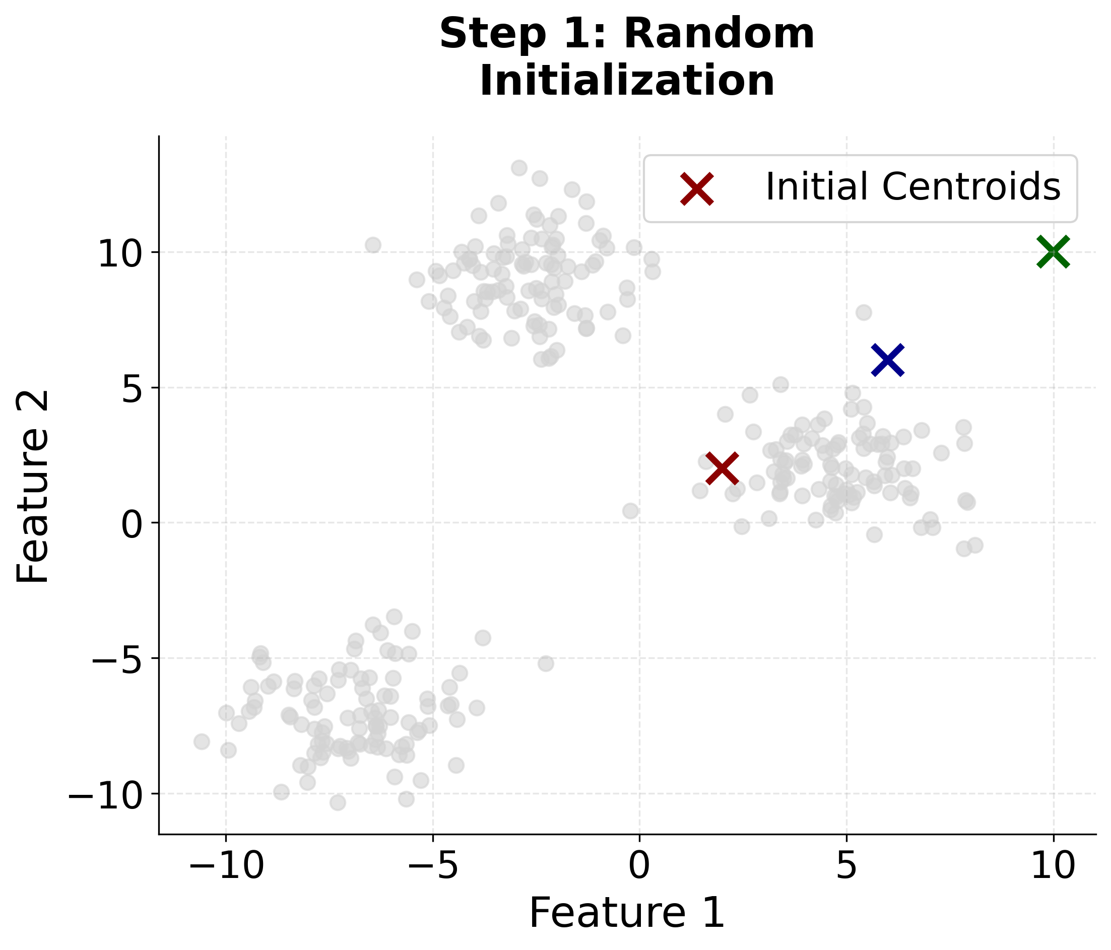
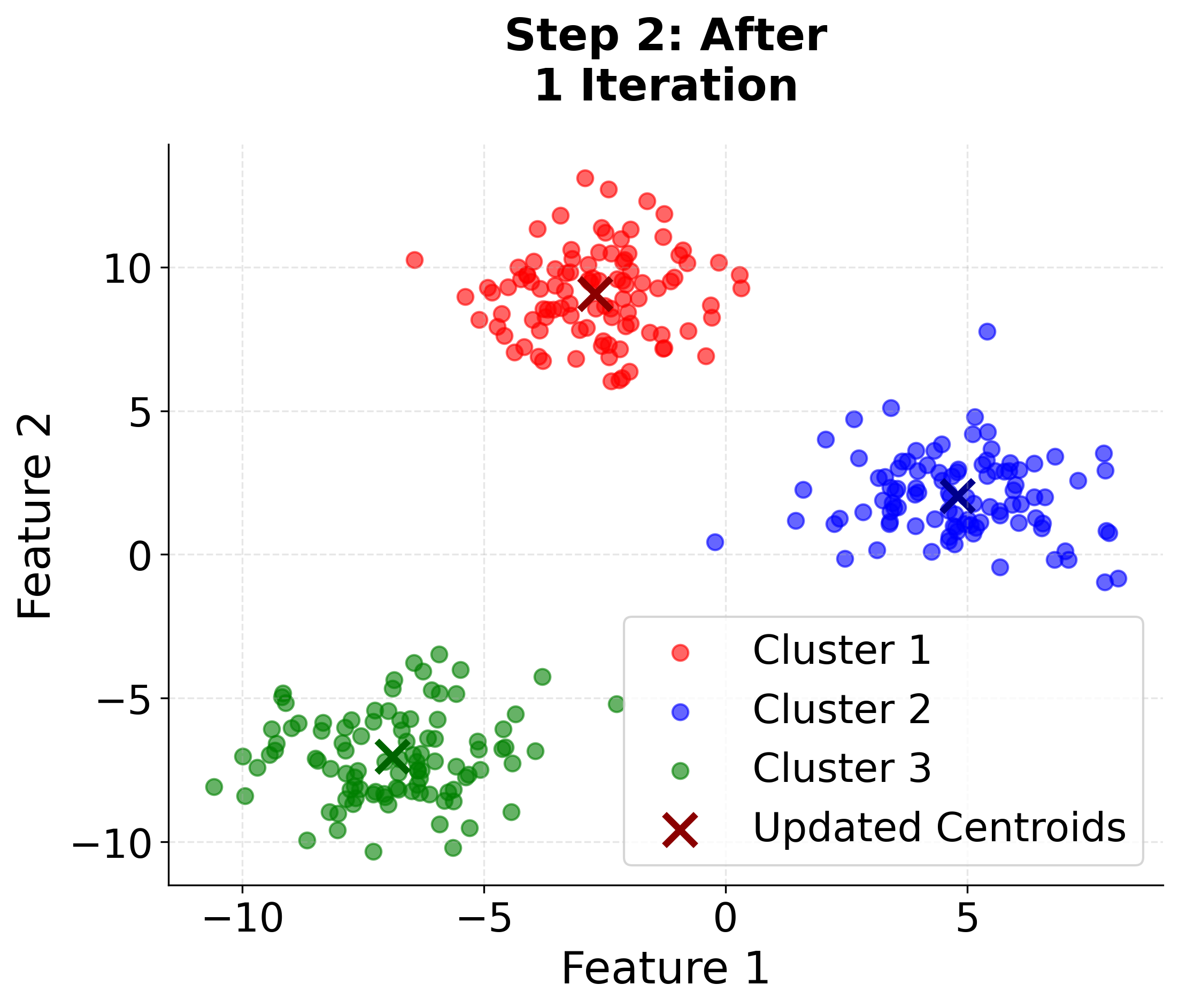
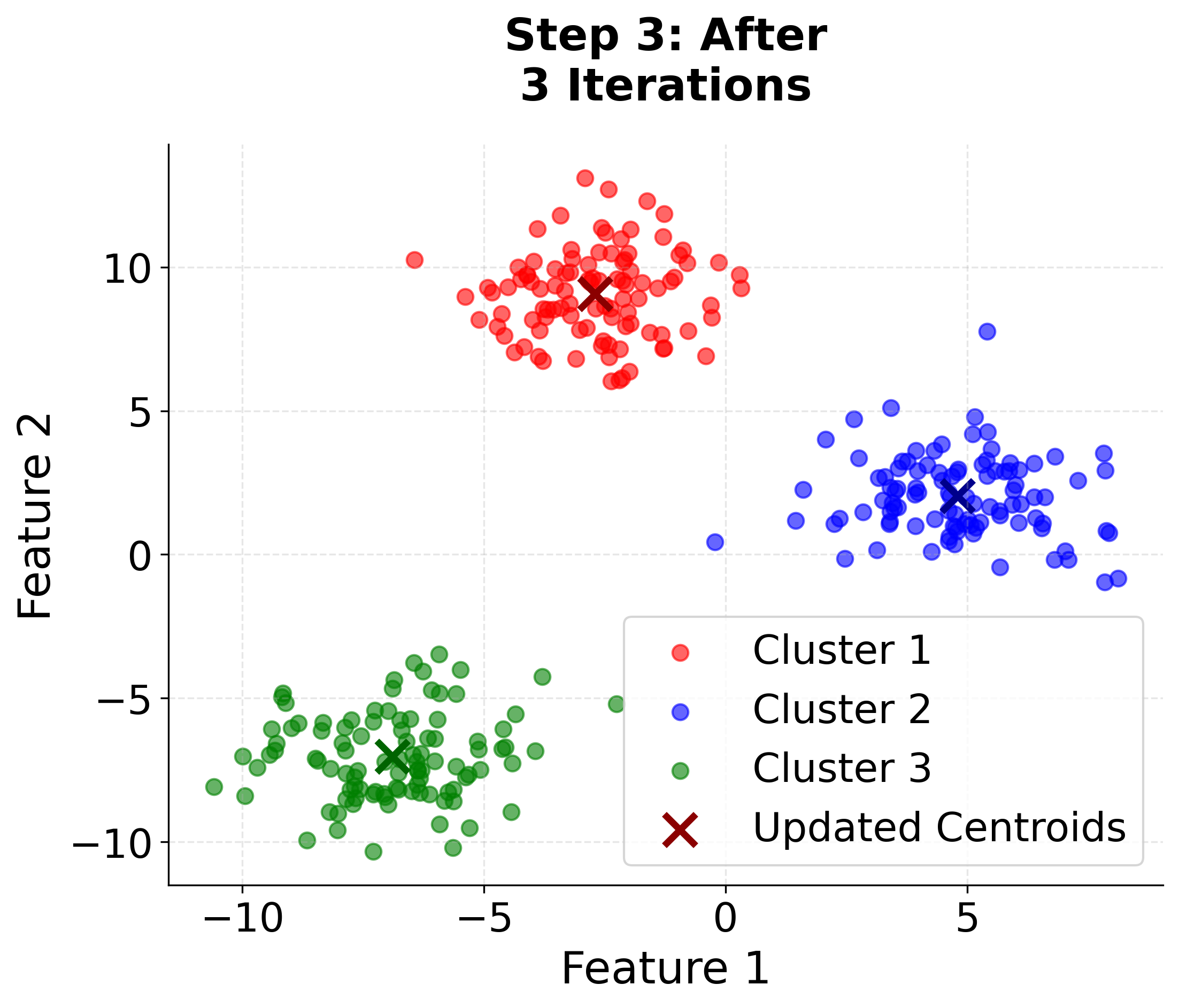
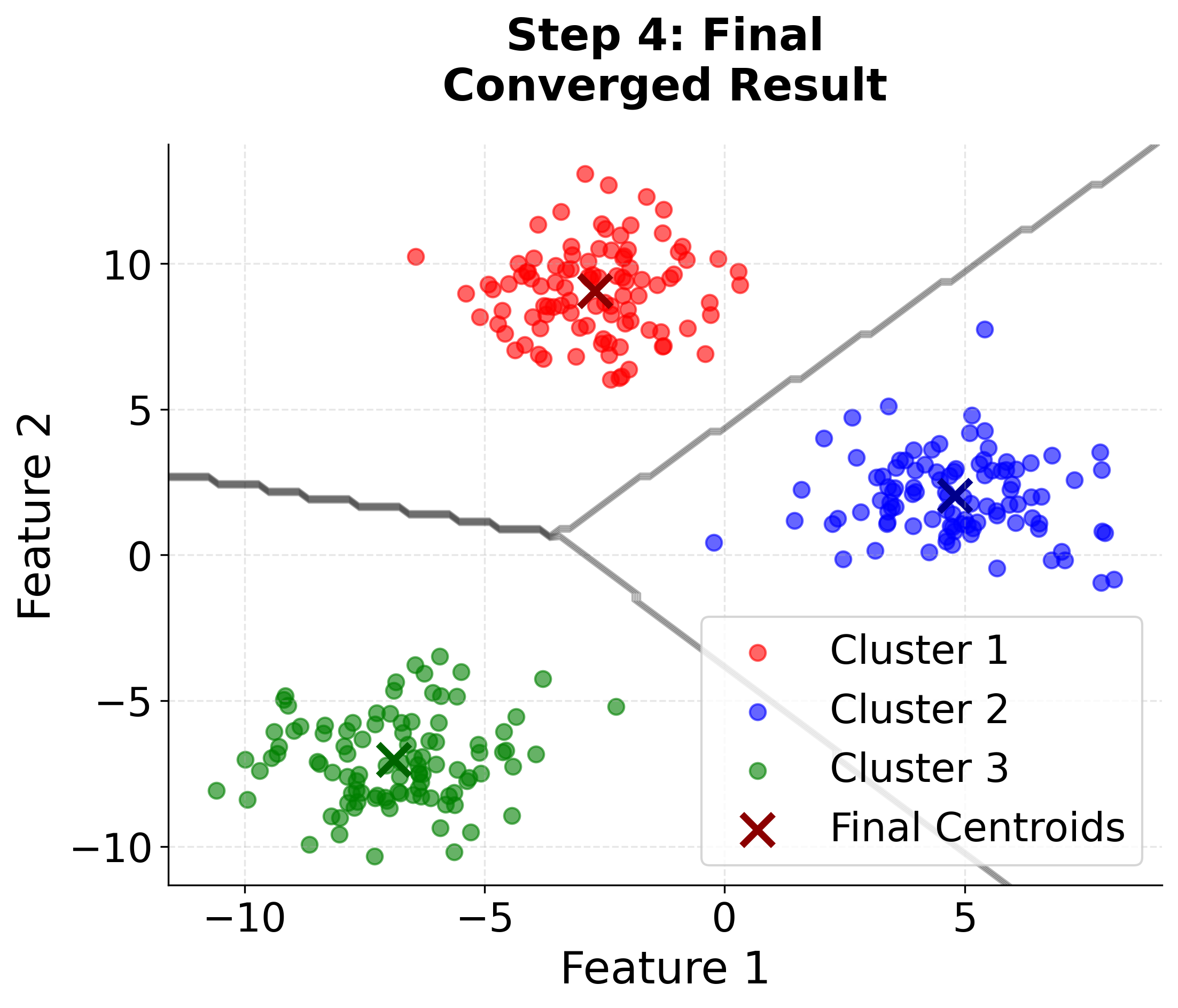
Here you can see the iterative nature of K-means clustering in action. Watch how the algorithm starts with random centroids and progressively improves the cluster assignments and centroid positions until convergence. The final plot includes cluster boundaries to show how the algorithm partitions the feature space.

Now let's create a second visualization that shows the impact of different initialization strategies and the importance of choosing the right number of clusters:

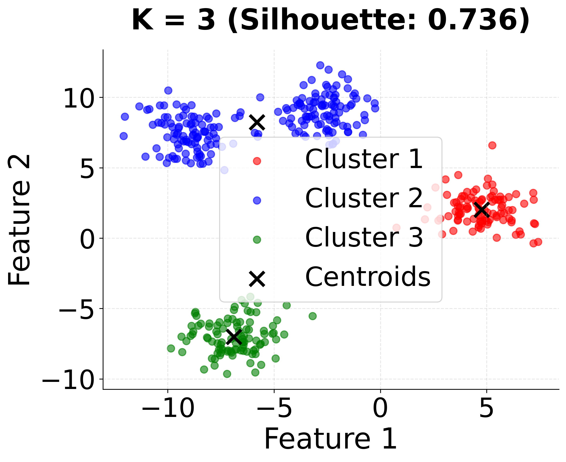
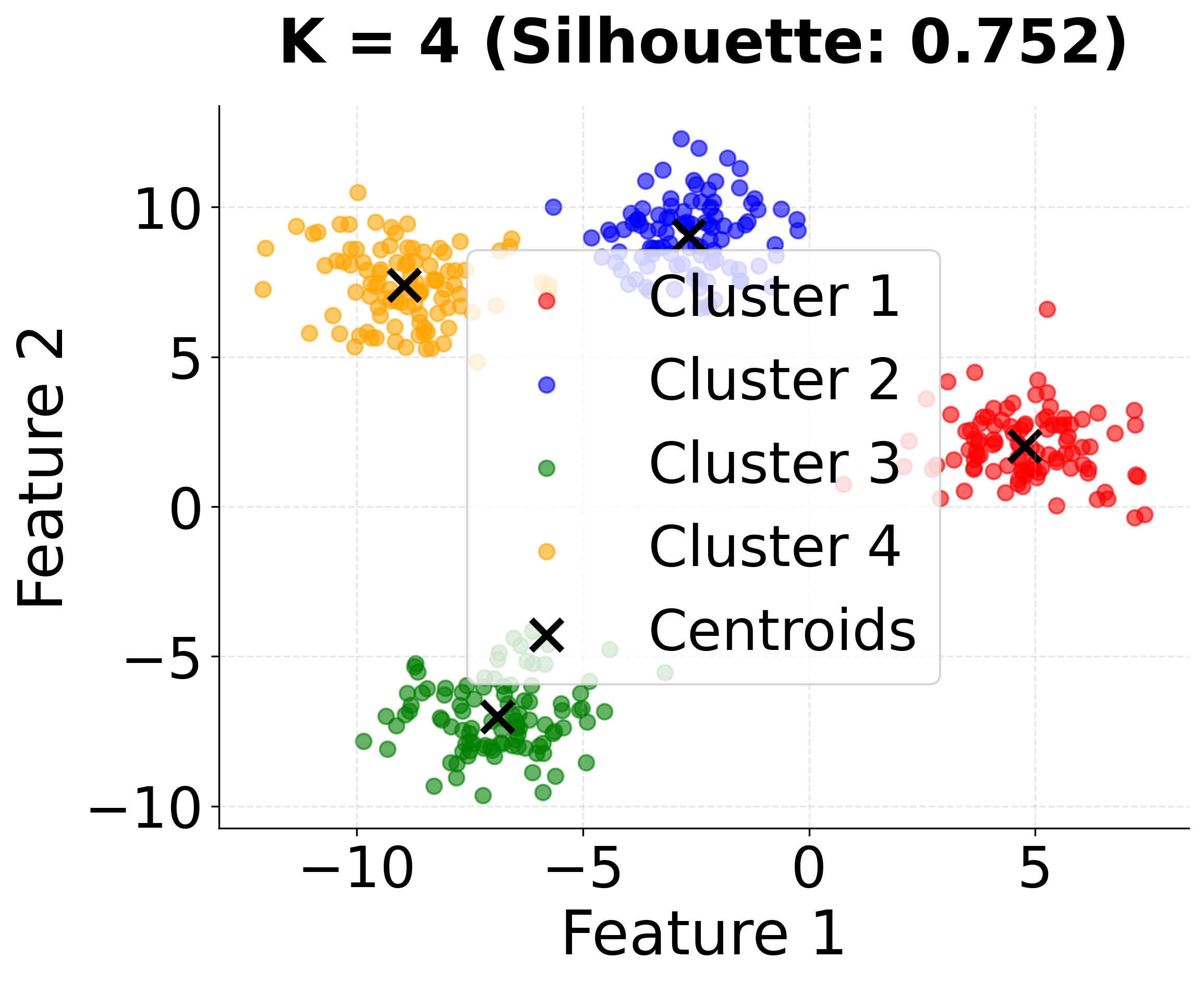
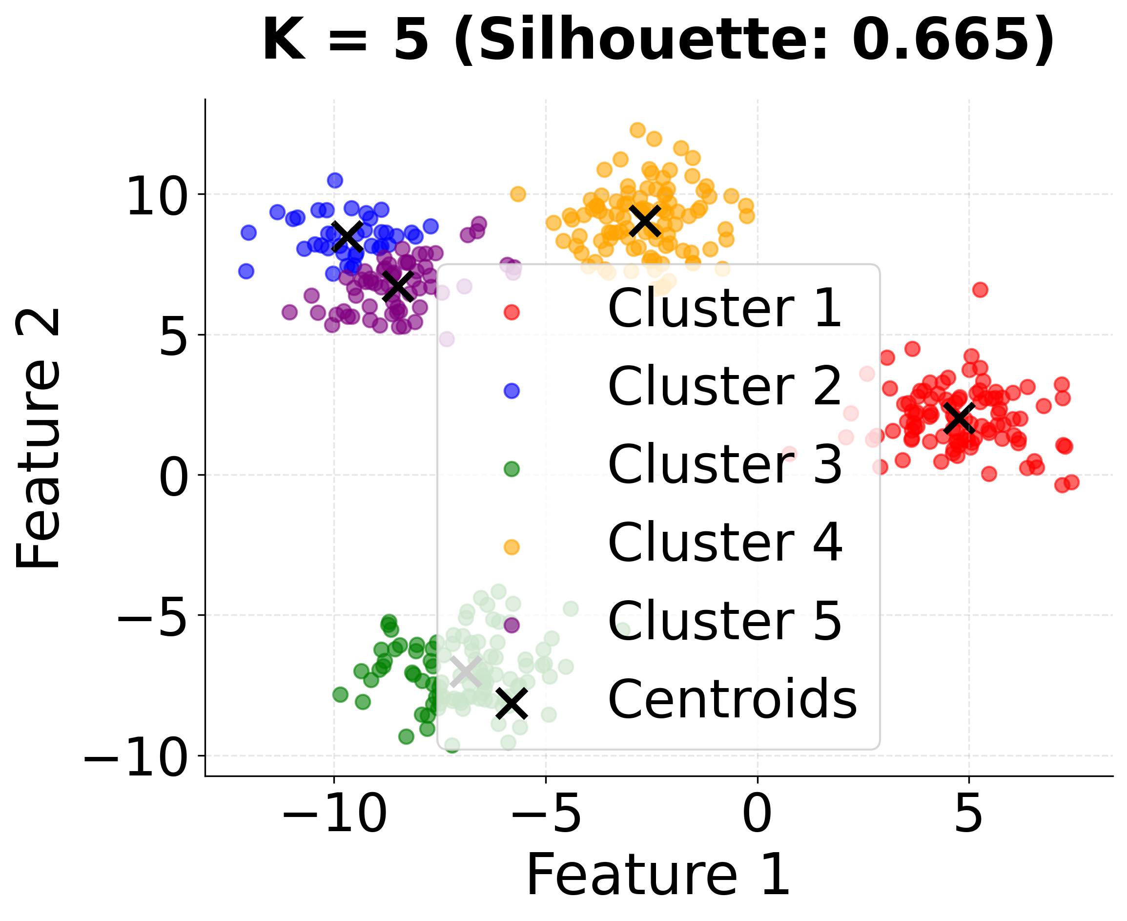
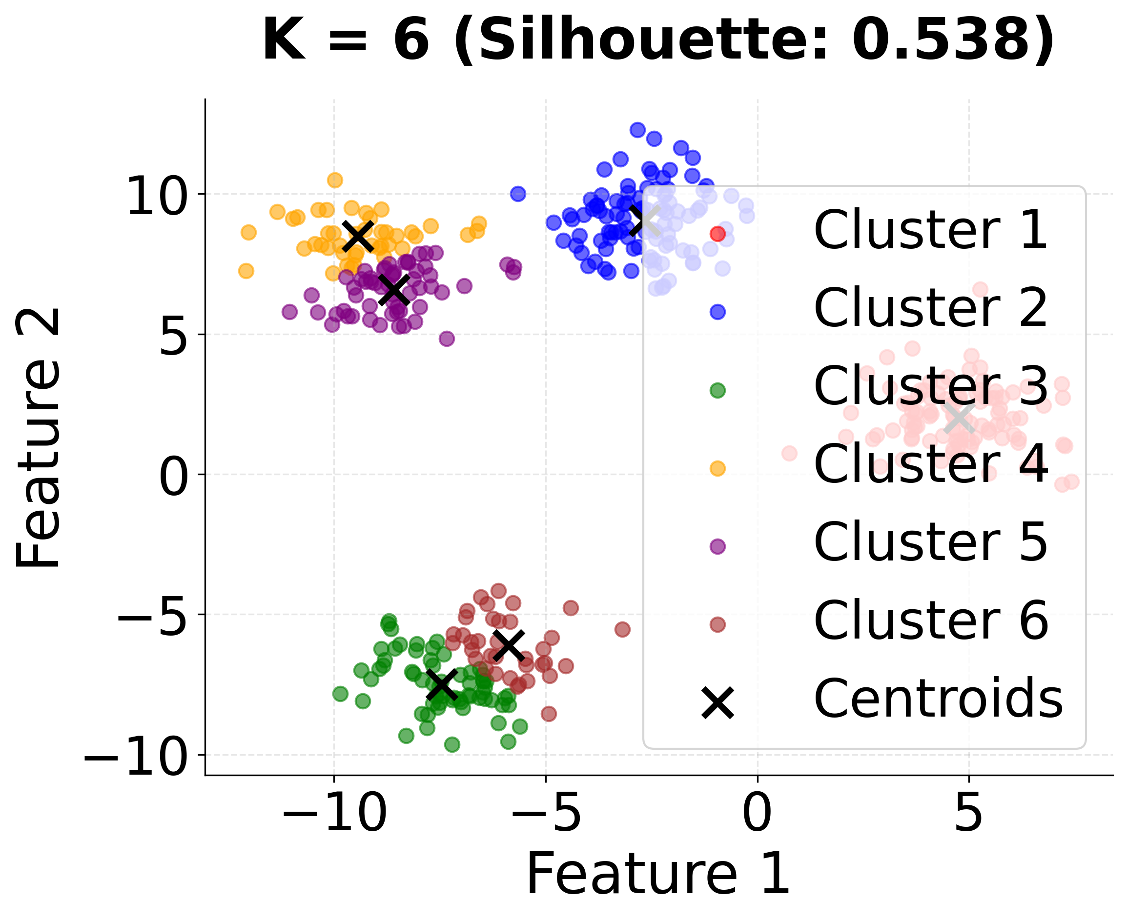
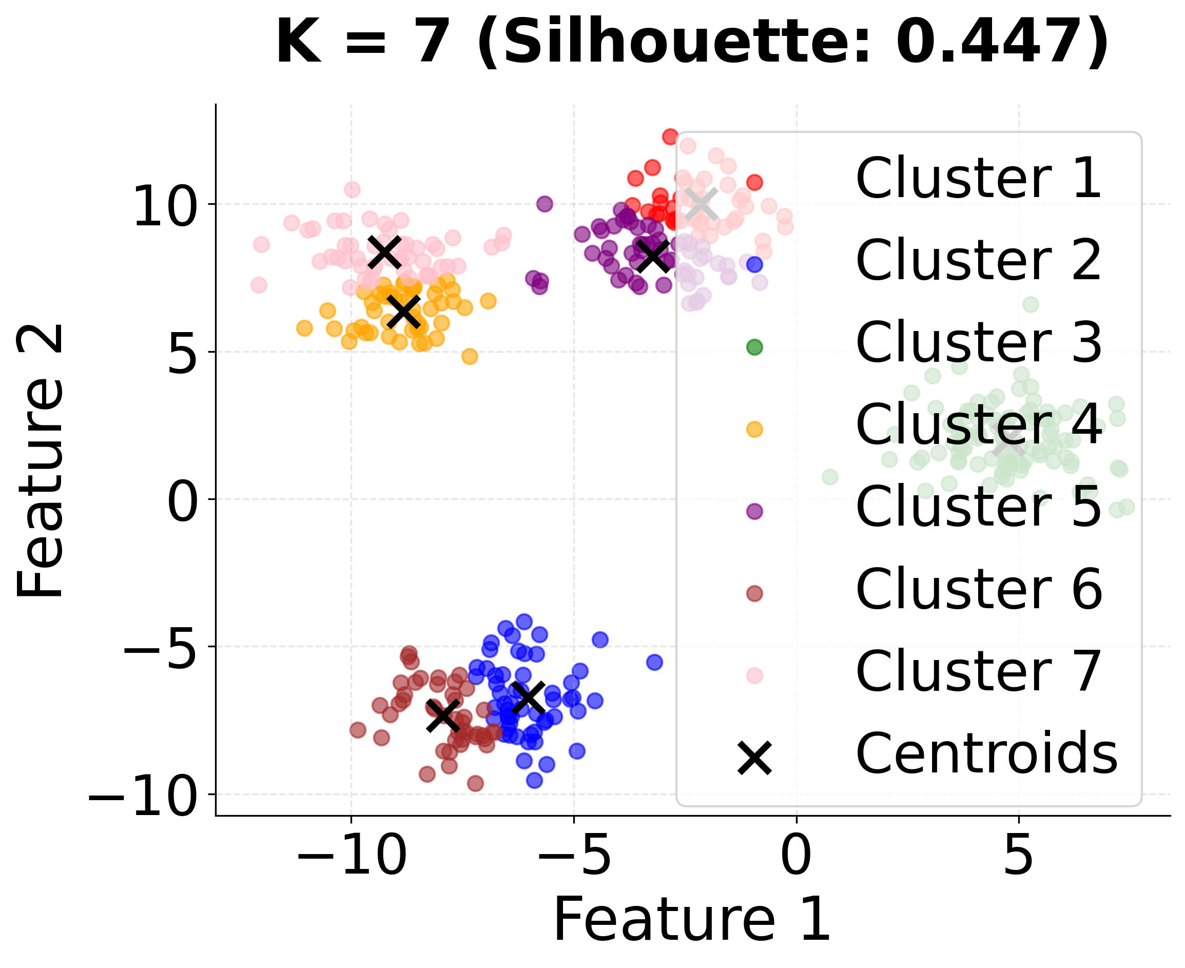
This second visualization shows how different values of k affect the clustering results. Notice that k=4 (the true number of clusters) achieves the highest silhouette score, demonstrating the importance of choosing the appropriate number of clusters.

Number of Clusters

One of the key challenges in K-means clustering is determining the optimal number of clusters k. Since the algorithm requires us to specify k beforehand, we need reliable methods to evaluate different values of k and select the best one. Two of the most widely-used methods are the elbow method and silhouette analysis.

The Elbow Method

The elbow method is based on the principle that as we increase the number of clusters k, the within-cluster sum of squares (WCSS) or inertia will decrease. However, the rate of decrease typically slows down after the optimal number of clusters, creating an "elbow" shape in the plot of k versus WCSS.

Mathematical Foundation

The Within-Cluster Sum of Squares (WCSS), also known as inertia, is a key metric used to evaluate the compactness of clusters formed by the K-means algorithm. It measures the total squared distance between each data point and the centroid of the cluster to which it has been assigned. The goal of K-means is to minimize this value, resulting in clusters where points are as close as possible to their respective centroids.

Mathematically, WCSS for a given number of clusters $k$ is defined as:

Where:

• $k$ is the number of clusters.
• $C_i$ denotes the set of data points assigned to the $i$-th cluster.
• $\mu_i$ is the centroid (mean vector) of the $i$-th cluster.
• $\|x - \mu_i\|^2$ is the squared Euclidean distance between a data point $x$ and the centroid $\mu_i$.

The WCSS value decreases as $k$ increases, because adding more clusters allows each cluster to be more compact. However, increasing $k$ indefinitely will eventually result in each data point being its own cluster, which is not useful for most applications.

The Elbow Criterion

The elbow method is a visual and intuitive technique for choosing the best number of clusters ($k$) in K-means clustering. Here’s how it works, step by step:

1. Plotting WCSS vs. $k$:
   For each possible value of $k$ (for example, from 1 to 10), you run K-means clustering and calculate the Within-Cluster Sum of Squares (WCSS). WCSS measures how tightly grouped the data points are within each cluster: the lower the WCSS, the more compact the clusters.

2. Looking for the "Elbow":
   You then plot the WCSS values on the y-axis against the number of clusters $k$ on the x-axis. As you increase $k$, WCSS will always decrease (or stay the same), because more clusters mean each cluster can be tighter. However, after a certain point, adding more clusters doesn't improve the WCSS by much. The plot typically looks like a bent arm, and the point where the curve bends sharply (like an elbow) is considered the optimal $k$.

3. Understanding the "Elbow" Mathematically:
   The "elbow" is the point where the rate at which WCSS decreases changes most dramatically. Before the elbow, adding clusters greatly reduces WCSS; after the elbow, the improvement is much smaller.

   To make this more precise, we can look at how WCSS changes as $k$ increases:

   • The first difference (similar to the first derivative in calculus) tells us how much WCSS drops when we add one more cluster:

     $$\text{Change at } k = \text{WCSS}(k) - \text{WCSS}(k+1)$$

     A large value means adding a cluster made a big difference; a small value means it didn’t help much.

   • The second difference (similar to the second derivative) tells us how the rate of improvement itself is changing. For discrete $k$, we estimate this using:

     $$\text{Second difference at } k \approx \text{WCSS}(k+1) - 2\,\text{WCSS}(k) + \text{WCSS}(k-1)$$

     The "elbow" is where this second difference is largest in absolute value, meaning the curve bends the most.

   In practice, you don't need to calculate derivatives. Most people simply look at the plot and pick the $k$ where the WCSS curve visibly flattens out (the point of diminishing returns).

To recapitulate all steps:

• Run K-means for a range of $k$ values (e.g., 1 to 10).
• Record the WCSS for each $k$.
• Plot WCSS versus $k$.
• Find the "elbow" (the point where adding more clusters doesn't reduce WCSS by much).

The elbow method helps you balance between having compact clusters (low WCSS) and keeping your model simple (not too many clusters). The "elbow" is the value of $k$ where adding more clusters yields only small improvements, so it’s a good choice for the number of clusters.

Keep in mind that sometimes the "elbow" is not very clear, and you may need to use your judgment or try other methods to confirm your choice.

Limitations of the Elbow Method

The elbow method has several limitations:

• The "elbow" is often subjective and not always clearly defined
• It may not work well when clusters have different sizes or densities
• The method assumes that the optimal k corresponds to a significant change in the WCSS curve
• It can be misleading when the data has a smooth, gradual decrease in WCSS

Let's visualize the elbow method in action:

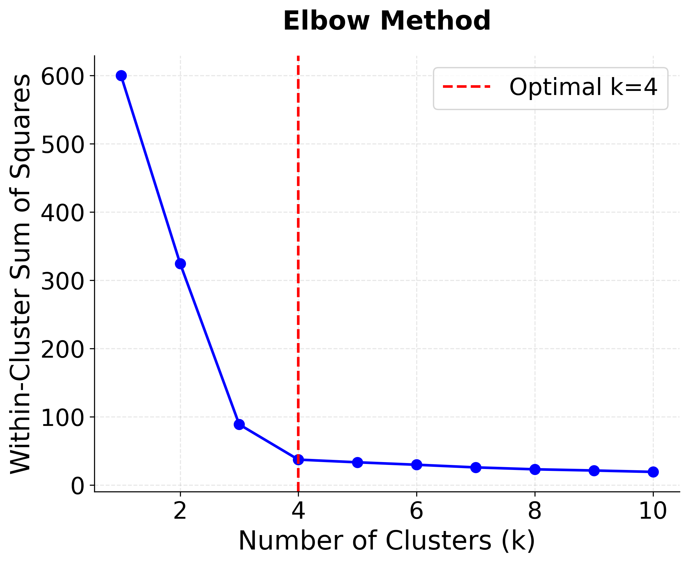
This visualization shows the characteristic "elbow" shape where the rate of decrease in WCSS slows down after k=4, indicating the optimal number of clusters. The red dashed line marks the true number of clusters in our synthetic data.

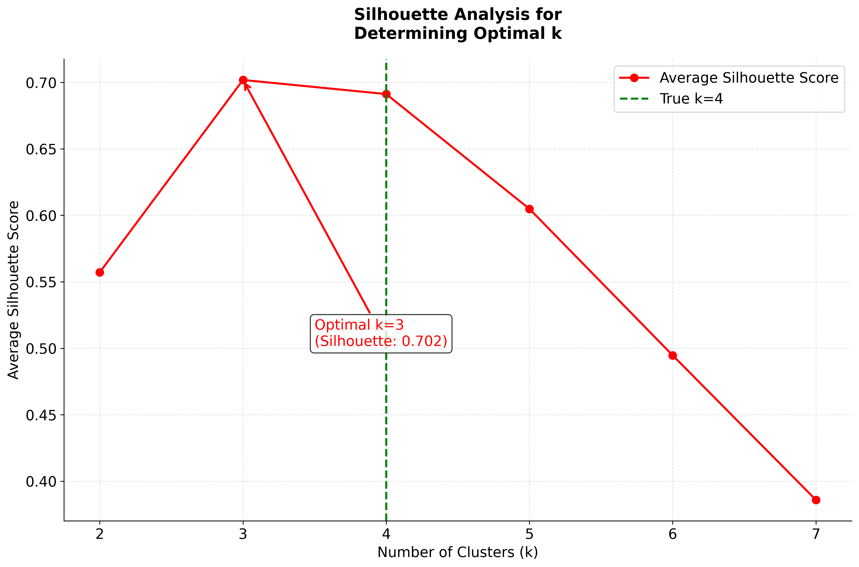
Silhouette Analysis

Silhouette analysis provides a more robust method for determining the optimal number of clusters by measuring how similar an object is to its own cluster compared to other clusters.

Mathematical Definition

For each data point i, the silhouette coefficient is calculated as:

$s(i) = \frac{b(i) - a(i)}{\max\{a(i), b(i)\}}$

Where:

• $a(i)$ is the average distance from point i to all other points in the same cluster (intra-cluster distance)
• $b(i)$ is the minimum average distance from point i to all points in any other cluster (inter-cluster distance)

Step-by-Step Calculation

Let's break down in detail how to calculate the silhouette coefficient for a single data point $x_i$:

1. Calculate the intra-cluster distance $a(i)$:

   The intra-cluster distance $a(i)$ measures how well $x_i$ is matched to its own cluster. It is defined as the average distance between $x_i$ and all other points in the same cluster $C_i$ (excluding $x_i$ itself):

   $$a(i) = \frac{1}{|C_i| - 1} \sum_{j \in C_i,\, j \neq i} \|x_i - x_j\|$$
   • $|C_i|$ is the number of points in cluster $C_i$.
   • The sum runs over all points $x_j$ in $C_i$ except $x_i$ itself.
   • $\|x_i - x_j\|$ denotes the distance (typically Euclidean) between $x_i$ and $x_j$.
   • If $x_i$ is the only point in its cluster, $a(i)$ is undefined, and the silhouette is not computed for that point.

2. Calculate the inter-cluster distance $b(i)$:

   The inter-cluster distance $b(i)$ quantifies how well $x_i$ would fit into its "neighbor" cluster, i.e., the next best cluster other than its own. For each cluster $C_k$ (where $C_k \neq C_i$), compute the average distance from $x_i$ to all points in $C_k$:

   $$d(i, C_k) = \frac{1}{|C_k|} \sum_{j \in C_k} \|x_i - x_j\|$$

   Then, $b(i)$ is the minimum of these average distances over all clusters $C_k$ not containing $x_i$:

   $$b(i) = \min_{C_k \neq C_i} d(i, C_k)$$
   • This means $b(i)$ is the average distance from $x_i$ to the nearest cluster it does not belong to.

3. Calculate the silhouette coefficient $s(i)$:

   The silhouette coefficient for $x_i$ combines $a(i)$ and $b(i)$ into a single value:

   $$s(i) = \frac{b(i) - a(i)}{\max\{a(i),\, b(i)\}}$$
   • $s(i)$ ranges from -1 to 1.
   • If $s(i)$ is close to 1, $x_i$ is much closer to its own cluster than to the next nearest cluster (well-clustered).
   • If $s(i)$ is close to 0, $x_i$ lies between two clusters.
   • If $s(i)$ is negative, $x_i$ is closer to another cluster than to its own (possibly misclassified).

Summary of Steps:

• For each data point $x_i$:
  1. Compute $a(i)$: average distance to all other points in the same cluster.
  2. Compute $b(i)$: lowest average distance to all points in any other cluster.
  3. Compute $s(i)$ using the formula above.

By repeating this process for every point in the dataset, you obtain a silhouette coefficient for each point, which can be averaged to assess the overall clustering quality.

Interpretation of Silhouette Values

The silhouette coefficient ranges from -1 to +1:

• $s(i) \approx 1$: Point i is well-clustered (much closer to its own cluster than to other clusters)
• $s(i) \approx 0$: Point i is on or very close to the decision boundary between clusters
• $s(i) \approx -1$: Point i is poorly clustered (closer to other clusters than to its own)

Average Silhouette Score

The overall quality of a clustering solution is measured by the average silhouette score:

$\text{Silhouette Score} = \frac{1}{n} \sum_{i=1}^{n} s(i)$

Where n is the total number of data points.

Choosing the Optimal k

To determine the optimal number of clusters:

1. Calculate the average silhouette score for different values of k
2. Choose the k that maximizes the average silhouette score
3. Additionally, examine the silhouette plot to ensure that most points have positive silhouette coefficients

Silhouette analysis offers several advantages when evaluating clustering results. It provides a clear, numerical measure of clustering quality, making it easier to assess how well the data has been grouped. This method is effective even when clusters vary in size and shape, and it offers valuable insight into the assignment of individual data points to clusters. Unlike the elbow method, silhouette analysis is less subjective, as it relies on a well-defined mathematical criterion. Additionally, it can help identify points that may be poorly clustered or potentially misclassified.

The silhouette coefficient possesses several important mathematical properties. It is always bounded between -1 and 1, ensuring interpretability. The coefficient is invariant to scaling and translation of the data, which means that the results are not affected by changes in the units or origin of the dataset. Furthermore, the silhouette score is independent of the number of clusters, allowing for meaningful comparisons between clustering solutions with different values of k. This makes it a versatile tool for evaluating and comparing various clustering outcomes.

Let's visualize silhouette analysis in action with both the score comparison and detailed silhouette plots for multiple k values:

Now let's create detailed silhouette plots for k=3, 4, and 5 to compare clustering quality:

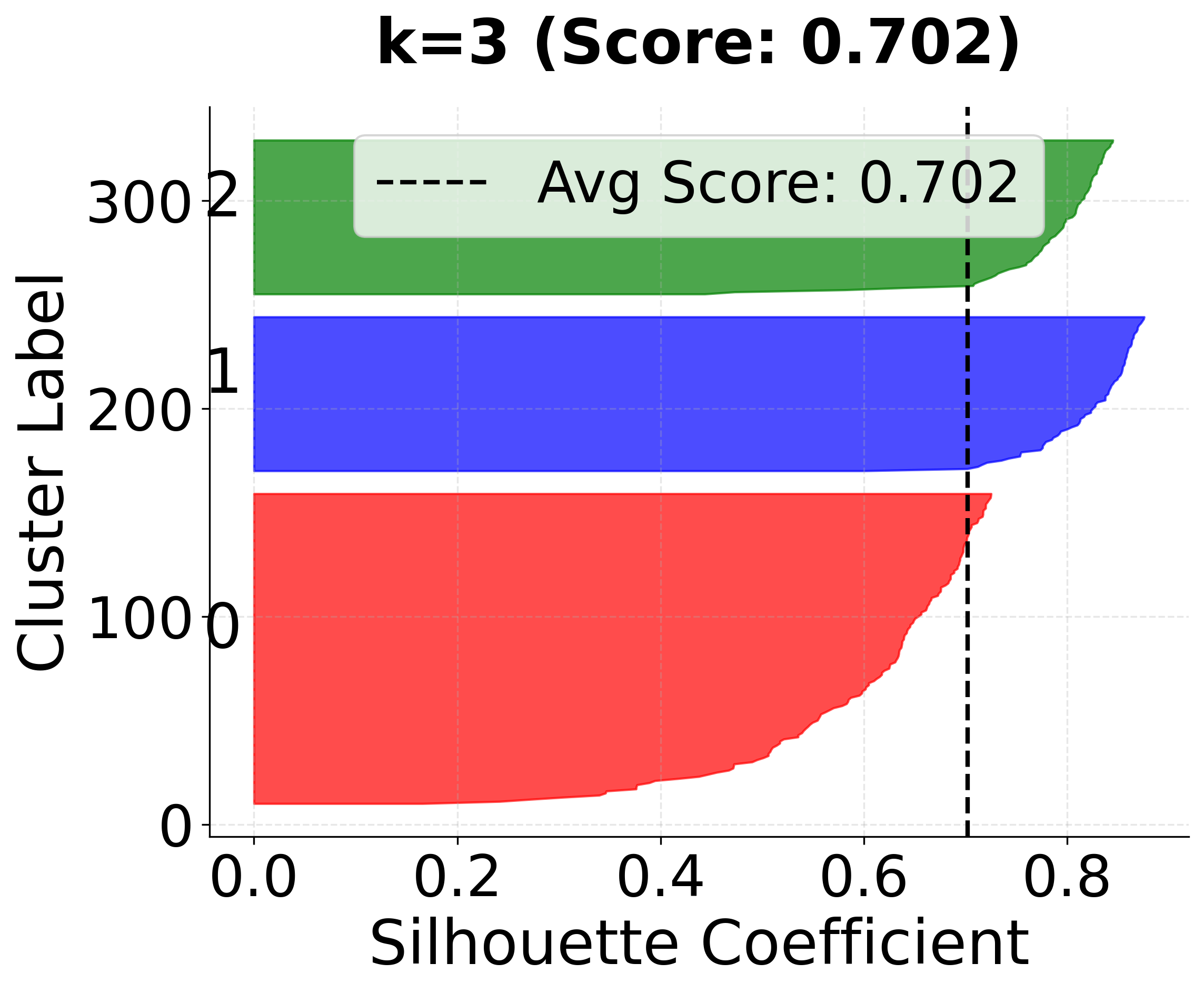
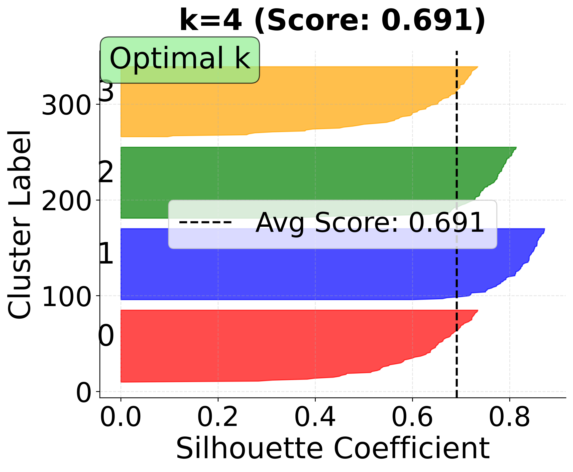
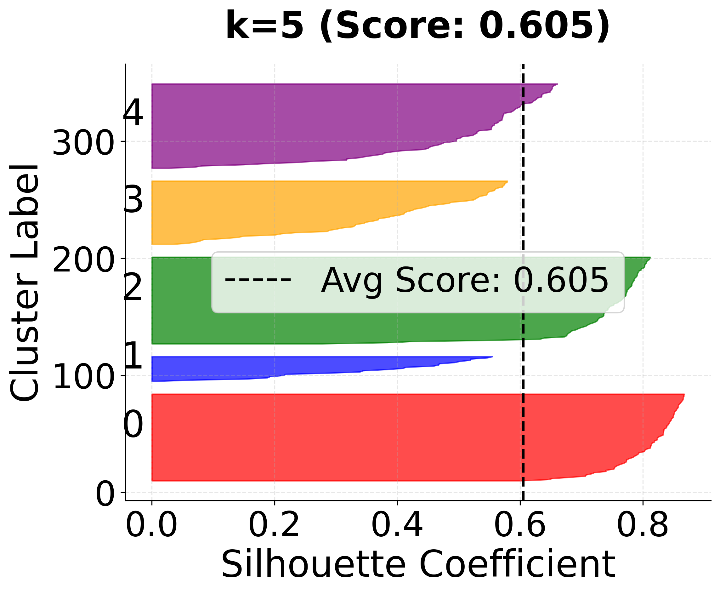
In this analysis, the silhouette score suggests that 3 clusters might be slightly better, but the elbow method and visual inspection of the charts for 4 clusters indicate that 4 clusters may provide a more meaningful grouping for real-world scenarios. This highlights the importance of combining quantitative metrics with domain intuition and visual inspection when selecting the optimal number of clusters.

Practical Guidelines for Interpretation

When deciding which method to use for determining the optimal number of clusters in K-means clustering, consider the characteristics of your dataset. The elbow method is most effective when you expect the clusters to be well-separated and clearly defined, as it identifies the point where adding more clusters yields diminishing returns in reducing within-cluster variance. In contrast, silhouette analysis tends to be more robust, especially for datasets with complex structures or clusters of varying shapes and sizes, as it evaluates how well each point fits within its assigned cluster compared to other clusters.

A practical approach is to combine both methods. Begin with the elbow method to obtain an initial estimate of the optimal number of clusters. Then, use silhouette analysis to validate and potentially refine this choice. It is also important to incorporate domain knowledge and consider any practical constraints relevant to your specific application. If the two methods suggest different values for the optimal number of clusters, silhouette analysis is generally considered more reliable due to its direct assessment of clustering quality.

Be mindful of certain warning signs during this process. If the elbow plot does not display a clear "elbow," the method may not be suitable for your data. Low average silhouette scores indicate that the clusters may not be well-separated, while negative silhouette coefficients suggest that some points may have been misclassified. In cases where the results are inconsistent or unsatisfactory, it may be necessary to revisit your data preprocessing steps or explore alternative clustering algorithms.

Example

Let's work through a concrete example of K-means clustering using a simple 2D dataset with 8 data points. This step-by-step calculation will help us understand exactly how the algorithm works.

Given Data Points: We have 8 points in 2D space:

• $A(1,\,1)$, $B(1,\,2)$, $C(2,\,1)$, $D(2,\,2)$
• $E(8,\,8)$, $F(8,\,9)$, $G(9,\,8)$, $H(9,\,9)$

We want to find $k=2$ clusters. Step 1: Initialization Let's randomly initialize two centroids:

• Centroid 1: $\mu_1 = (1.5,\ 1.5)$
• Centroid 2: $\mu_2 = (8.5,\ 8.5)$

Step 2: Assignment Step (First Iteration) For each point, we calculate the distance to both centroids and assign it to the nearest one.

For point $A(1, 1)$:

• Distance to $\mu_1$: $\sqrt{(1-1.5)^2 + (1-1.5)^2} = \sqrt{0.25 + 0.25} = \sqrt{0.5} \approx 0.707$
• Distance to $\mu_2$: $\sqrt{(1-8.5)^2 + (1-8.5)^2} = \sqrt{56.25 + 56.25} = \sqrt{112.5} \approx 10.61$
• $A$ is assigned to Cluster 1 (closer to $\mu_1$)

For point $E(8, 8)$:

• Distance to $\mu_1$: $\sqrt{(8-1.5)^2 + (8-1.5)^2} = \sqrt{42.25 + 42.25} = \sqrt{84.5} \approx 9.19$
• Distance to $\mu_2$: $\sqrt{(8-8.5)^2 + (8-8.5)^2} = \sqrt{0.25 + 0.25} = \sqrt{0.5} \approx 0.707$
• $E$ is assigned to Cluster 2 (closer to $\mu_2$)

Continuing this process for all points:

• Cluster 1: $A(1,1)$, $B(1,2)$, $C(2,1)$, $D(2,2)$
• Cluster 2: $E(8,8)$, $F(8,9)$, $G(9,8)$, $H(9,9)$

Step 3: Update Step (First Iteration)
Now we recalculate the centroids as the mean of points in each cluster.

For Cluster 1:
$\mu_1 = \left( \frac{1+1+2+2}{4},\ \frac{1+2+1+2}{4} \right) = (1.5,\ 1.5)$

For Cluster 2:
$\mu_2 = \left( \frac{8+8+9+9}{4},\ \frac{8+9+8+9}{4} \right) = (8.5,\ 8.5)$

Step 4: Convergence Check
The centroids haven't changed, so the algorithm has converged!

Final Result:

• Cluster 1: $\{A, B, C, D\}$ with centroid $(1.5,\ 1.5)$
• Cluster 2: $\{E, F, G, H\}$ with centroid $(8.5,\ 8.5)$

Verification:
Let's verify that no point would change clusters if we reassigned them:

• All points in Cluster 1 are closer to $(1.5,\ 1.5)$ than to $(8.5,\ 8.5)$
• All points in Cluster 2 are closer to $(8.5,\ 8.5)$ than to $(1.5,\ 1.5)$

The algorithm has successfully identified two distinct clusters in our data.

Let's visualize this step-by-step example to see how the algorithm works:

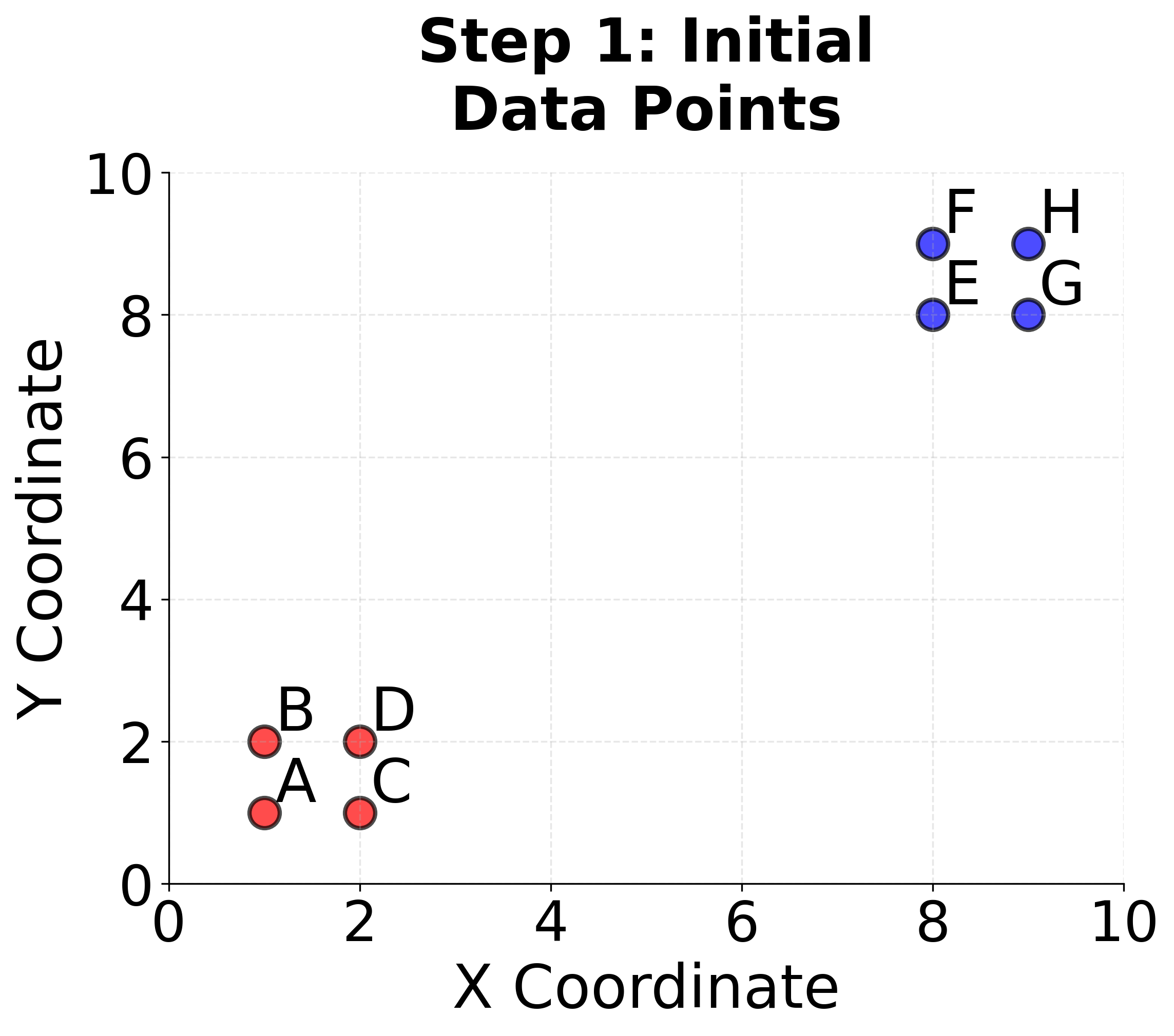
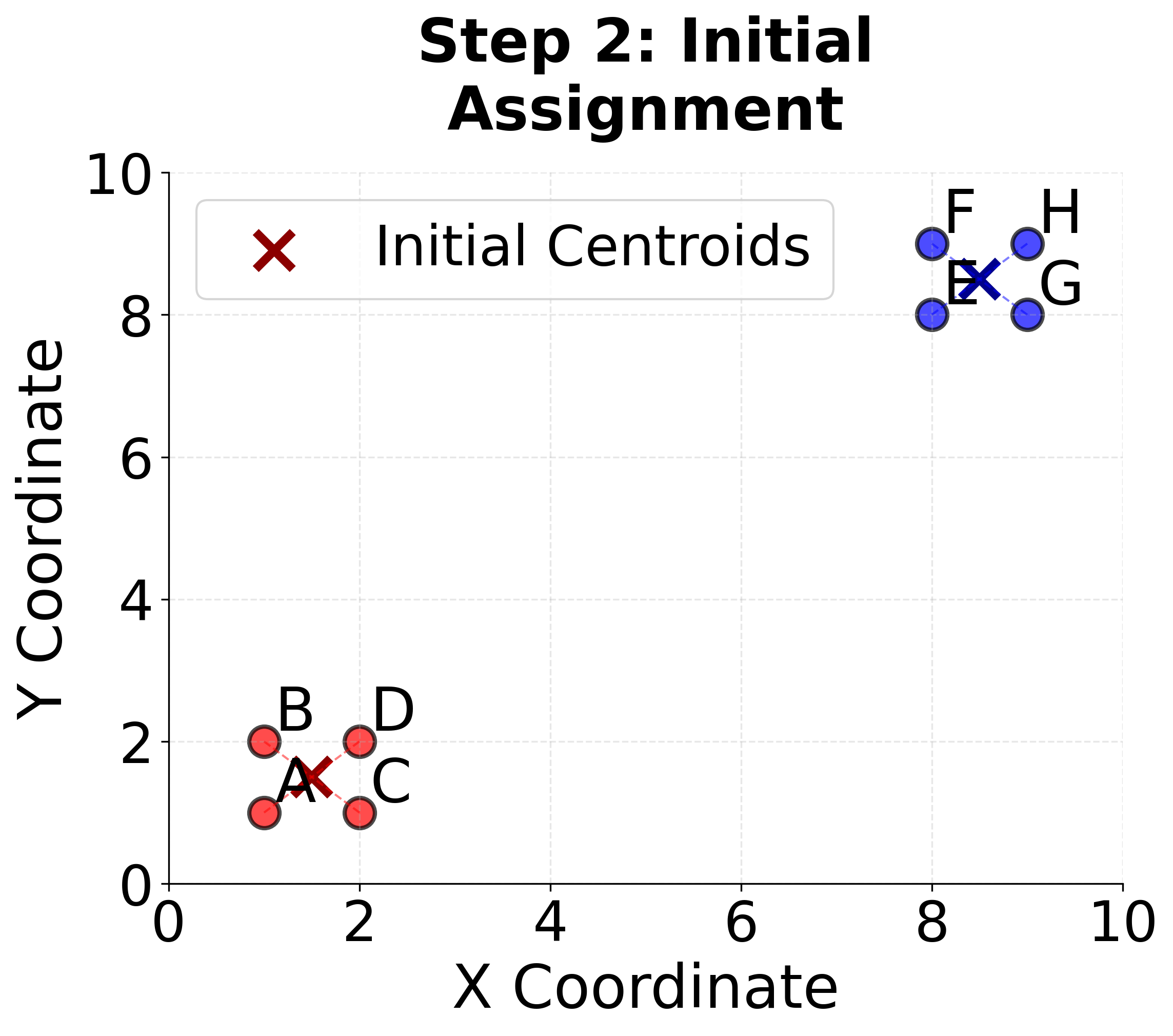
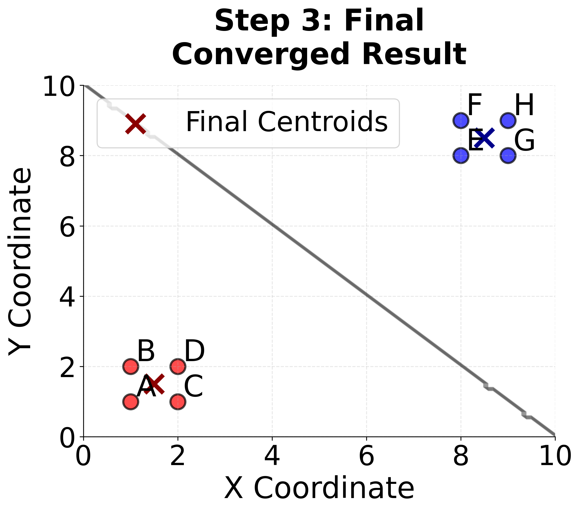
Here you can see the complete K-means process on our simple 8-point example, showing how the algorithm successfully identifies the two natural clusters in the data.

In this example we've chosen random initial centroids that conveniently were located in the middle of the two clusters to make the example simple. In practice, we should use the k-means++ initialization method to choose the initial centroids.

K-means++ Initialization

One of the key aspects of K-means clustering is the initialization of cluster centroids. Poor initialization can lead to suboptimal clustering results, convergence to local minima, and inconsistent outcomes across different runs. The K-means++ initialization algorithm addresses these issues by providing a smart, probabilistic approach to selecting initial centroids.

The Problem with Random Initialization

Traditional random initialization has several significant drawbacks:

1. Poor Local Minima: Random centroids may be placed in regions that lead to suboptimal clustering solutions
2. Inconsistent Results: Different random initializations can produce vastly different clustering results
3. Slow Convergence: Poor initial centroids may require many iterations to converge
4. Sensitivity to Outliers: Random initialization doesn't account for the distribution of data points

The K-means++ Algorithm

K-means++ is an intelligent initialization method that selects initial centroids based on the distribution of data points. The algorithm ensures that centroids are well-spread across the data space, reducing the likelihood of poor local minima and improving clustering quality.

Step-by-Step K-means++ Initialization:

1. First Centroid: Randomly select the first centroid from the dataset
2. Distance Calculation: For each remaining data point, calculate the squared distance to the nearest already-selected centroid
3. Probability Assignment: Assign each point a probability proportional to its squared distance to the nearest centroid
4. Weighted Selection: Select the next centroid randomly, but with probability proportional to the squared distances
5. Repeat: Continue steps 2-4 until k centroids are selected

Mathematical Formulation:

Let $D(x)$ be the shortest distance from a data point $x$ to the closest centroid already chosen. The probability of selecting point $x$ as the next centroid is:

$P(x) = \frac{D(x)^2}{\sum_{i=1}^{n} D(x_i)^2}$

Where:

• $D(x)^2$ is the squared distance from point $x$ to its nearest centroid
• The denominator is the sum of squared distances for all points
• This ensures points far from existing centroids have higher selection probability

K-means++ offers several important advantages over traditional random initialization. By ensuring that initial centroids are well-distributed throughout the data space, K-means++ typically leads to improved clustering quality. This careful placement of centroids not only enhances the final clustering results but also allows the algorithm to converge more quickly, often requiring fewer iterations to reach a stable solution.

Another benefit of K-means++ is its reduced sensitivity to the choice of random seed. Because the initialization process is guided by the distribution of the data, the results are more consistent across different runs, making the algorithm more reliable in practice.

From a theoretical perspective, K-means++ provides strong guarantees: it achieves an $O(\log k)$ approximation to the optimal K-means solution. This means that, in addition to its practical benefits, K-means++ is also supported by solid mathematical foundations.

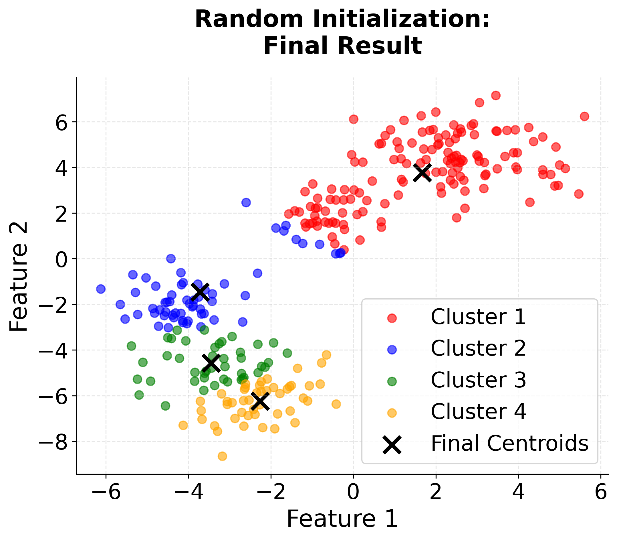
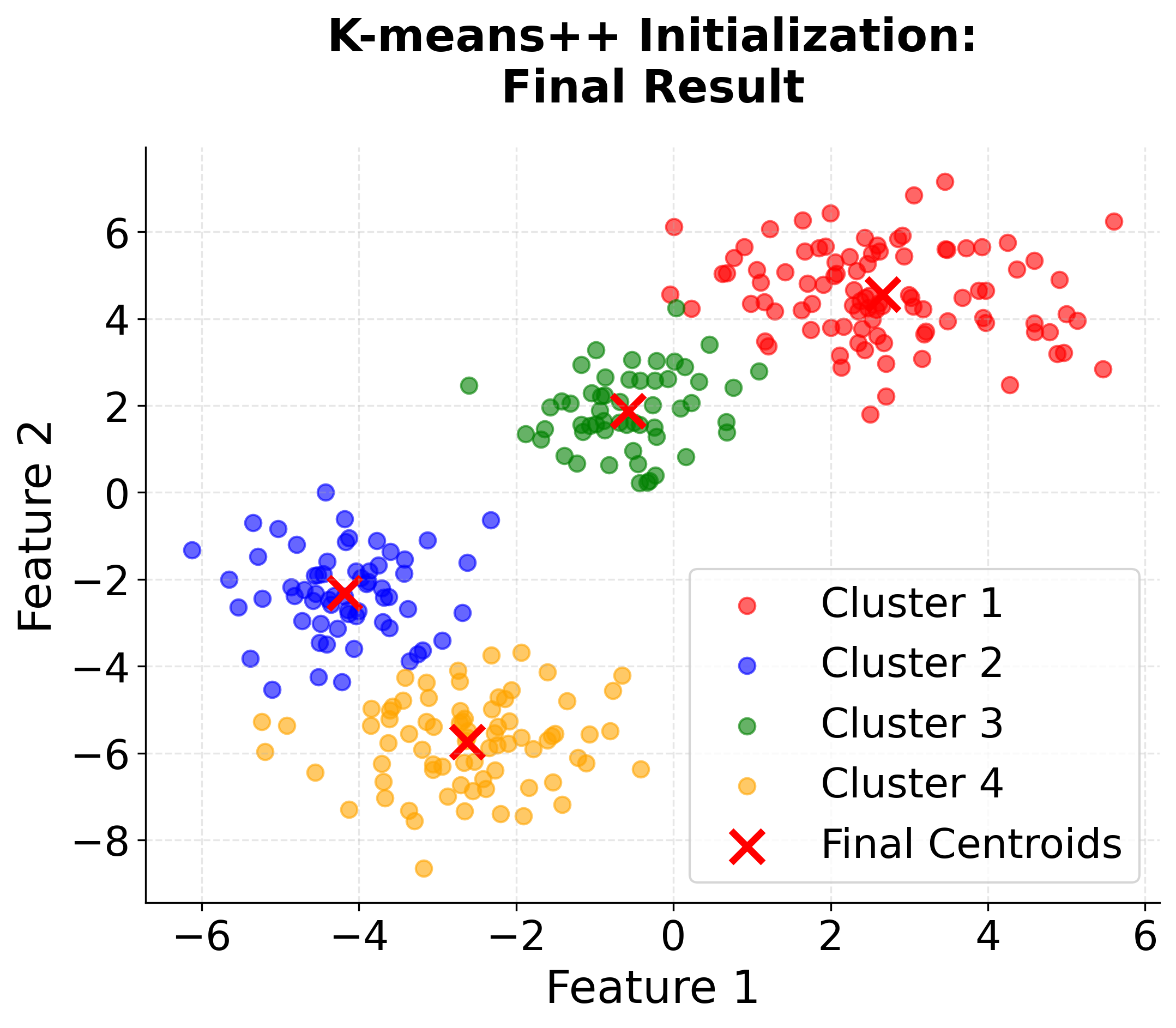
Visualizing K-means++ vs Random Initialization

Let's create a visualization that demonstrates the difference between random initialization and K-means++ initialization:

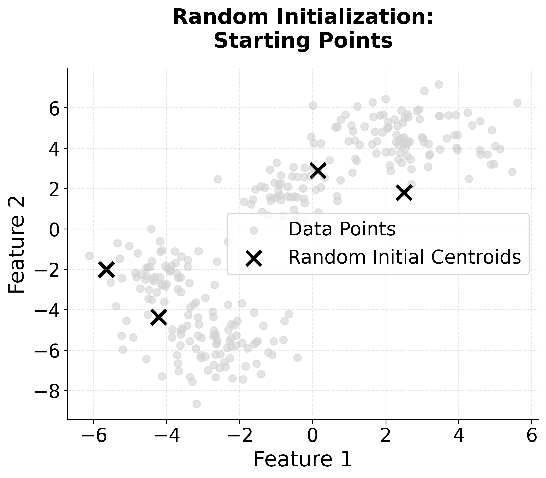
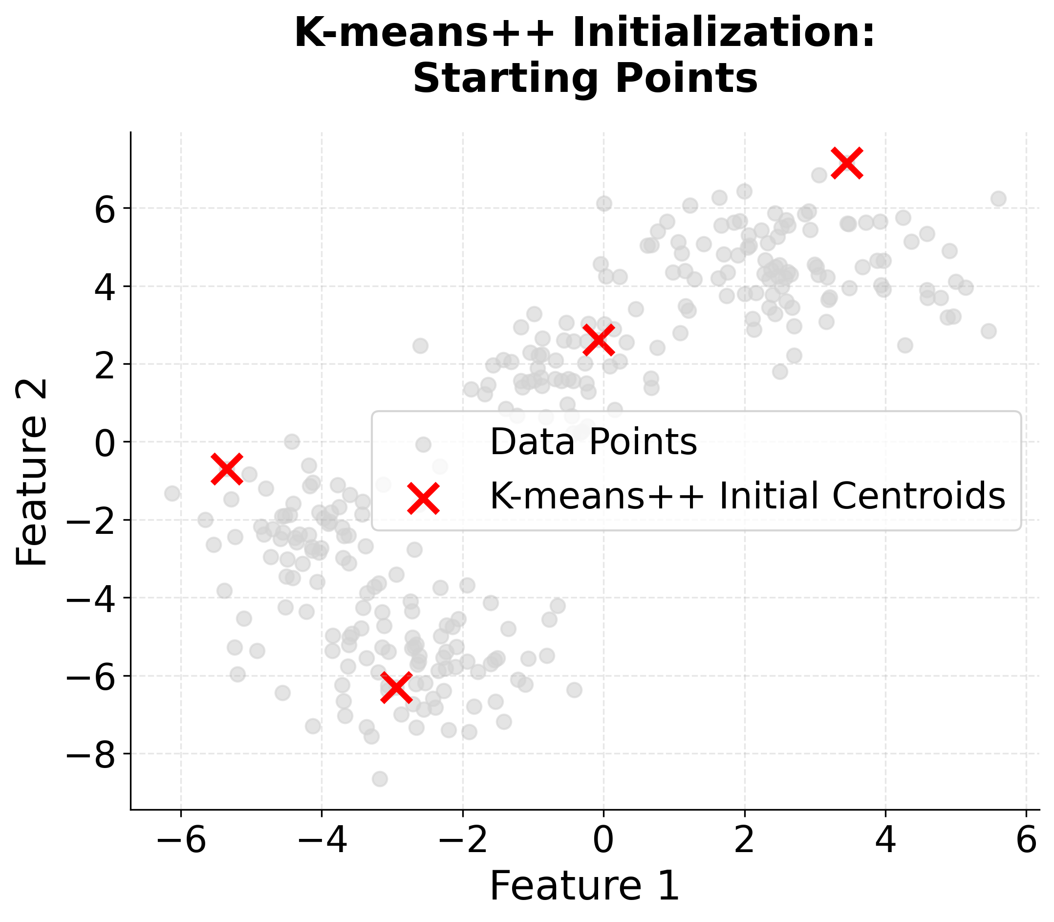
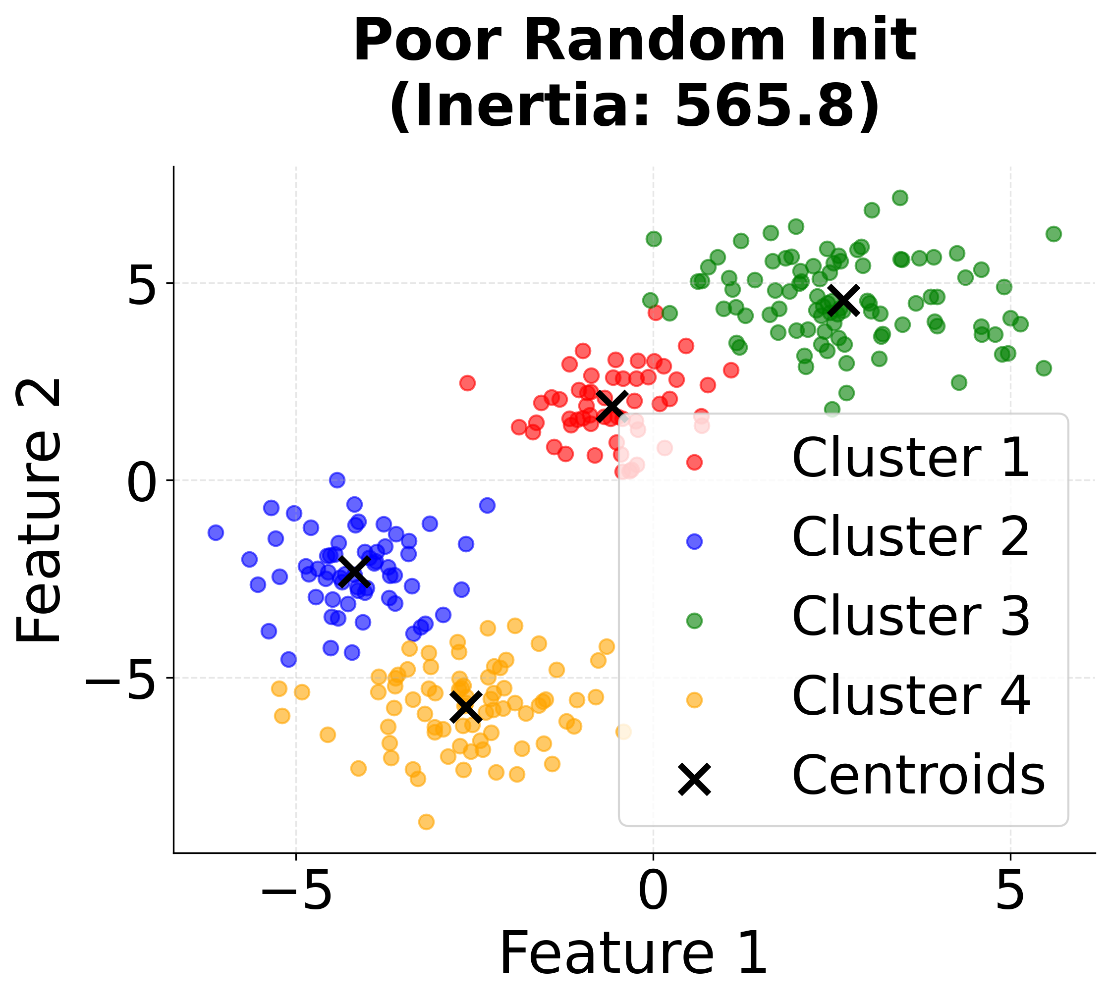
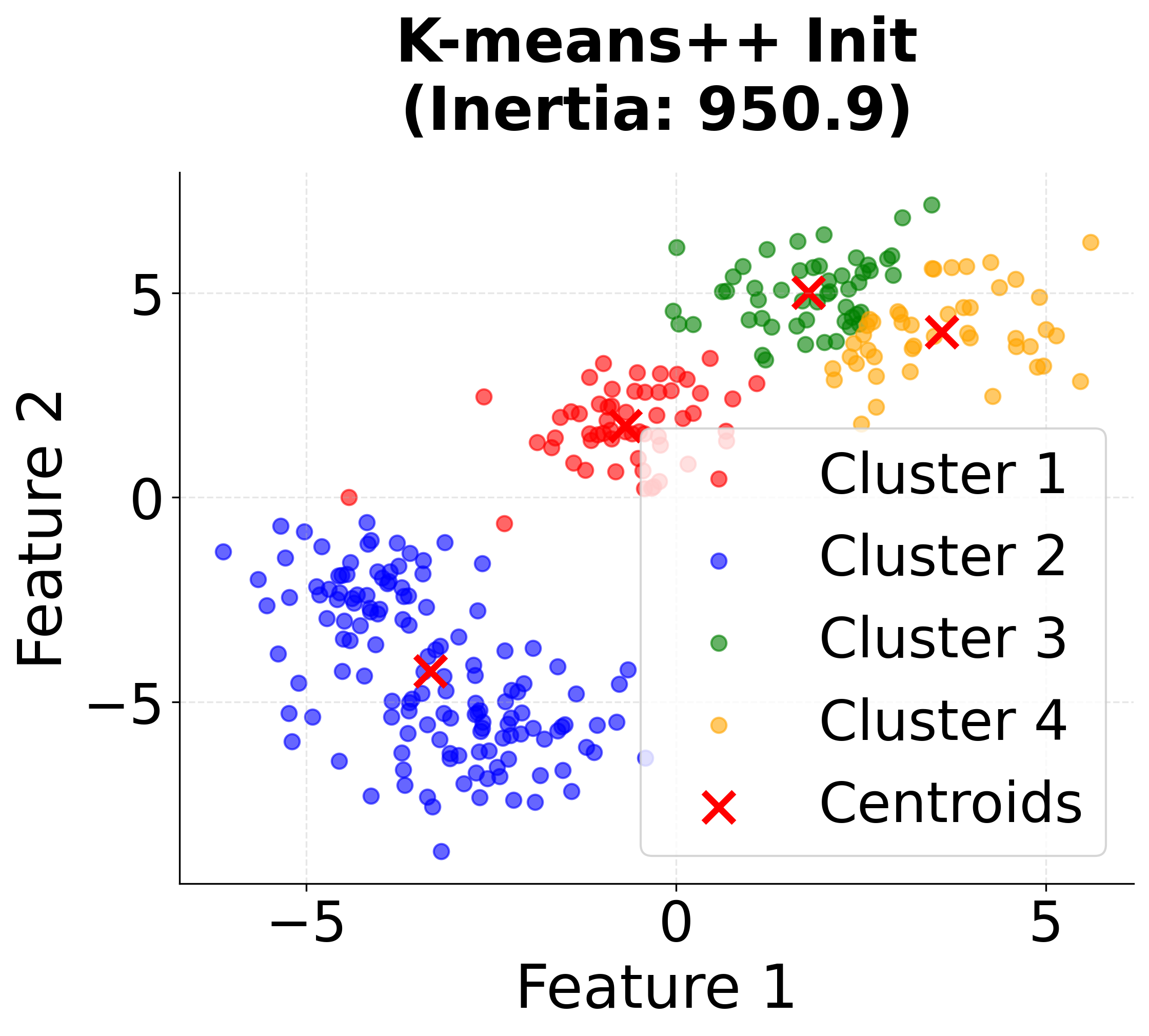
When to Use K-means++

K-means++ initialization is widely regarded as the best default choice for initializing centroids in K-means clustering. In most applications, it consistently yields better clustering results than random initialization, and it does so with only a modest increase in computational cost. This advantage becomes especially pronounced when working with large datasets, where random initialization is more likely to result in poor local minima and suboptimal clustering.

The benefits of K-means++ are even more significant in high-dimensional data. As the number of features increases, the risk of poor initial centroid placement with random initialization grows, making the careful, data-aware selection of initial centroids by K-means++ even more valuable. In production environments, where reliable and consistent clustering outcomes are essential, K-means++ provides the robustness and repeatability needed for dependable results.

From a computational perspective, K-means++ initialization has a time complexity of $O(nkd)$, where $n$ is the number of data points, $k$ is the number of clusters, and $d$ is the number of features. Although this is higher than the $O(kd)$ complexity of random initialization, the extra cost is typically negligible because initialization is performed only once, and the improvement in clustering quality and convergence speed usually outweighs the additional computation.

To get the most out of K-means++ initialization, several best practices should be followed. First, it is advisable to use K-means++ as the default initialization method unless there is a compelling reason to choose otherwise. Second, even with K-means++, running the algorithm multiple times (by setting n_init > 1) is recommended to further reduce the risk of poor local minima and to select the best clustering result. Third, set a random state for reproducibility, which is particularly important in research and production settings. Finally, ensure that your data is properly scaled before applying K-means++, as the algorithm is sensitive to differences in feature scales.

In summary, K-means++ initialization offers a substantial improvement over random initialization, leading to more robust, consistent, and higher-quality clustering results. A solid understanding and correct implementation of this initialization strategy are important for achieving optimal performance with K-means clustering.

Implementation

This section provides a comprehensive, step-by-step tutorial for implementing K-means clustering using scikit-learn. We'll work through a complete example that demonstrates data preparation, model fitting, evaluation, and optimization techniques.

Step 1: Data Preparation and Setup

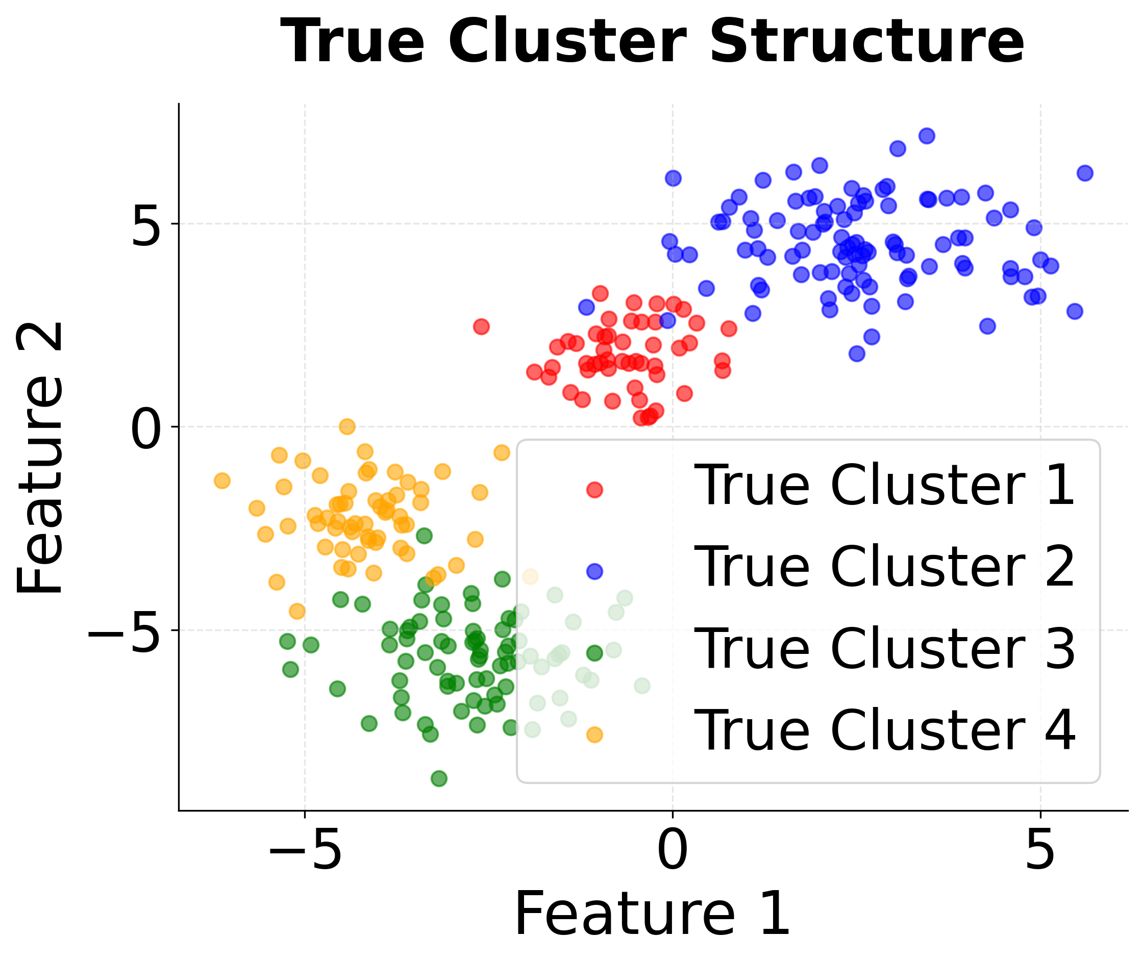
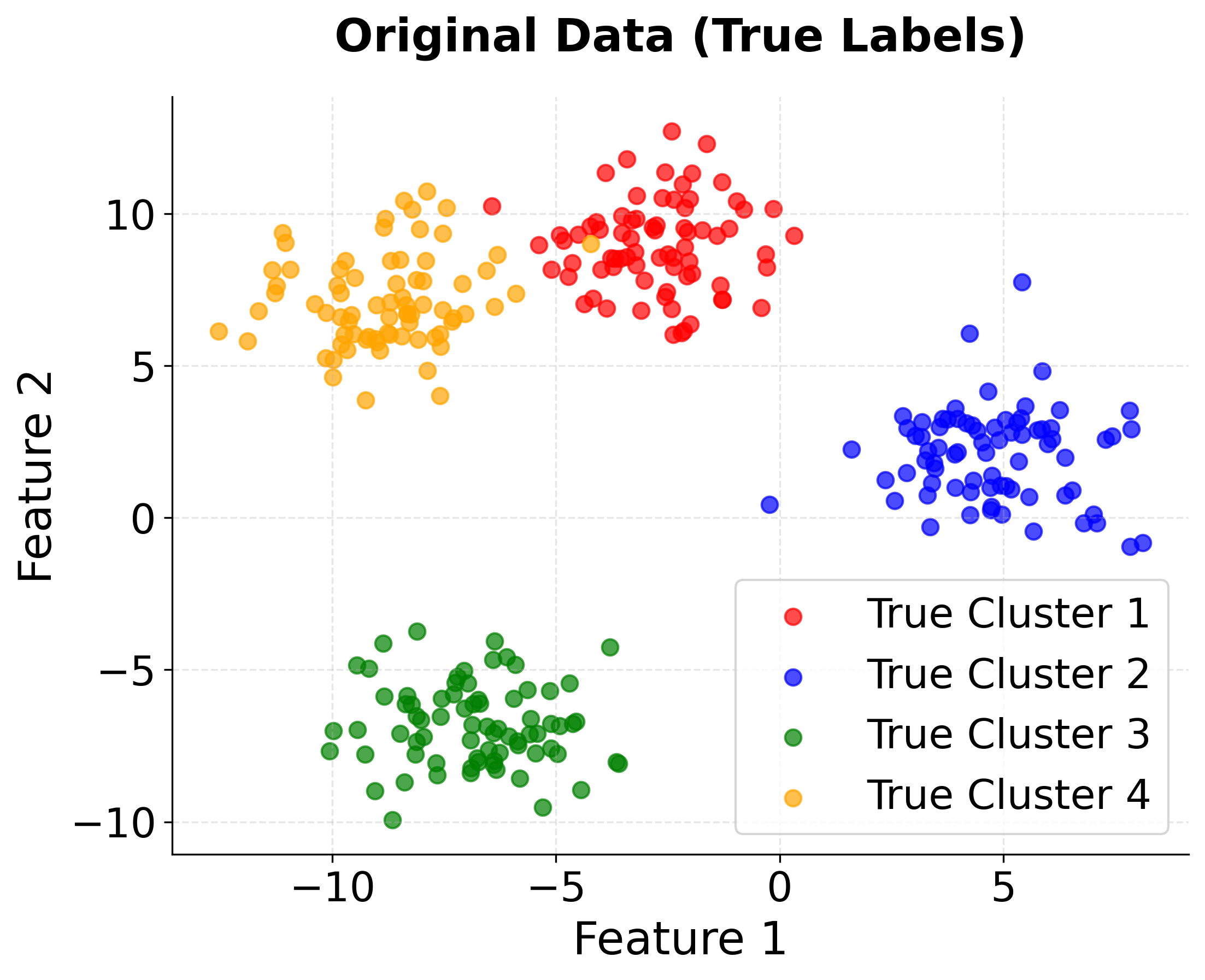
First, we'll import the necessary libraries and create a synthetic dataset with known cluster structure. This allows us to validate our implementation against ground truth.

The dataset contains 300 samples with 2 features, organized into 4 natural clusters. Standardization ensures that both features contribute equally to the distance calculations, preventing features with larger scales from dominating the clustering process.

The output confirms our data setup is correct. The shape shows we have 300 data points with 2 features, and the 4 unique cluster labels match our synthetic data generation parameters. This provides a solid foundation for testing K-means clustering.

Step 2: Basic K-means Implementation

Now we'll implement K-means clustering with the known optimal number of clusters. The algorithm will iteratively assign points to clusters and update centroids until convergence.

The n_init=10 parameter runs the algorithm 10 times with different random initializations and selects the best result, helping avoid poor local optima. The algorithm converged quickly, indicating well-separated clusters.

These results indicate good algorithm performance. The number of iterations shows how quickly the algorithm converged, which provides insight into cluster separation. The inertia value provides a baseline for comparing different clustering solutions, and the centroids shape confirms we have 4 cluster centers in our 2-dimensional feature space.

Step 3: Clustering Quality Evaluation

We'll evaluate the clustering performance using multiple metrics to get a comprehensive assessment of the results.

• Silhouette Score: Values above 0.6 indicate strong, well-separated clusters. This score shows that data points are much closer to their own cluster than to other clusters.
• Adjusted Rand Index: Values close to 1.0 show near-perfect agreement with true labels, indicating the algorithm successfully recovered the underlying cluster structure.
• Inertia: The within-cluster sum of squares provides a baseline for comparison with other k values.

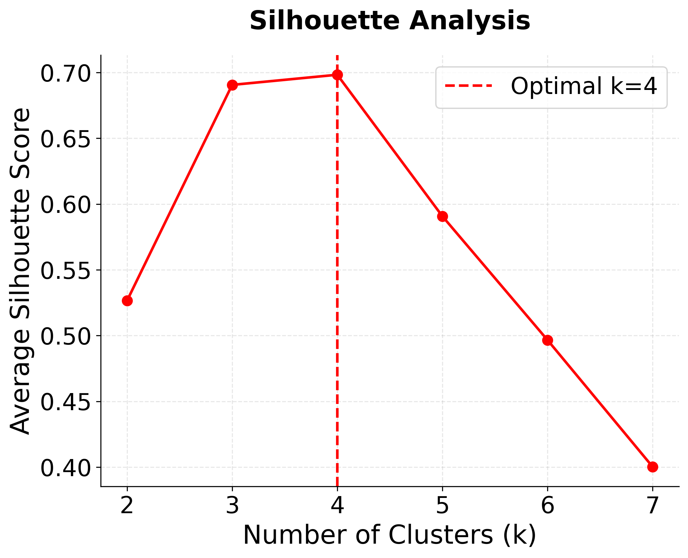
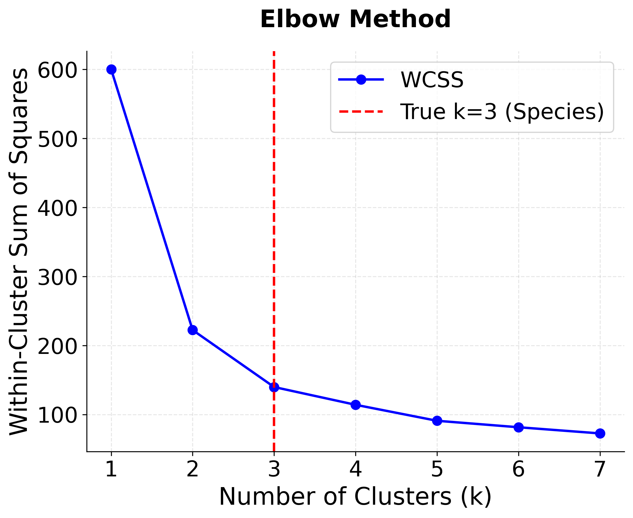
Step 4: Finding the Optimal Number of Clusters

In practice, we often don't know the true number of clusters. Let's demonstrate how to determine the optimal k using systematic evaluation.

The results clearly show that k=4 is optimal:

• Inertia decreases monotonically with increasing k, but the rate of decrease slows after k=4, indicating diminishing returns
• Silhouette score peaks at k=4, confirming this as the best choice for cluster separation
• Performance degrades for k>4 as we over-cluster the data, creating artificial subdivisions that don't reflect the true structure

Step 5: Comprehensive Visualization

Let's create a comprehensive visualization that shows our clustering results and validation methods. This will help us understand both the clustering quality and the effectiveness of our optimization techniques.

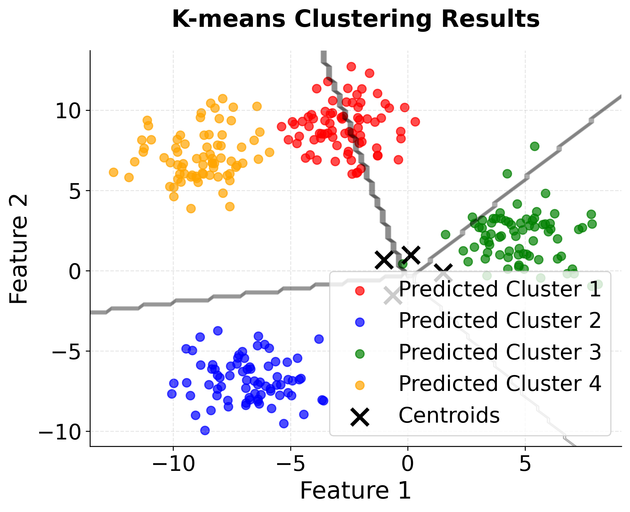
You can see how the visualizations confirm our numerical results:

• Perfect cluster separation in the original data makes this an ideal test case
• K-means successfully recovers the true cluster structure with minimal misclassification
• Clear elbow at k=4 in the WCSS plot validates our choice of optimal clusters
• Peak silhouette score at k=4 provides additional confirmation of optimal clustering

Step 5: Real-World Example - Iris Dataset

Now let's apply K-means to a real dataset to demonstrate practical considerations. The Iris dataset contains measurements of three flower species, providing a classic clustering challenge.

The results show moderate clustering performance:

• Silhouette Score: Moderate quality, indicating some overlap between clusters. This is lower than our synthetic data because real-world data has natural variation and boundary cases.
• Adjusted Rand Index: Strong agreement with true species labels, showing the algorithm captures the main species structure despite some misclassification.
• Uneven cluster sizes: The algorithm finds slightly different cluster sizes than the true 50-50-50 distribution, reflecting the natural overlap between some species.

Step 6: Optimizing k for Real Data

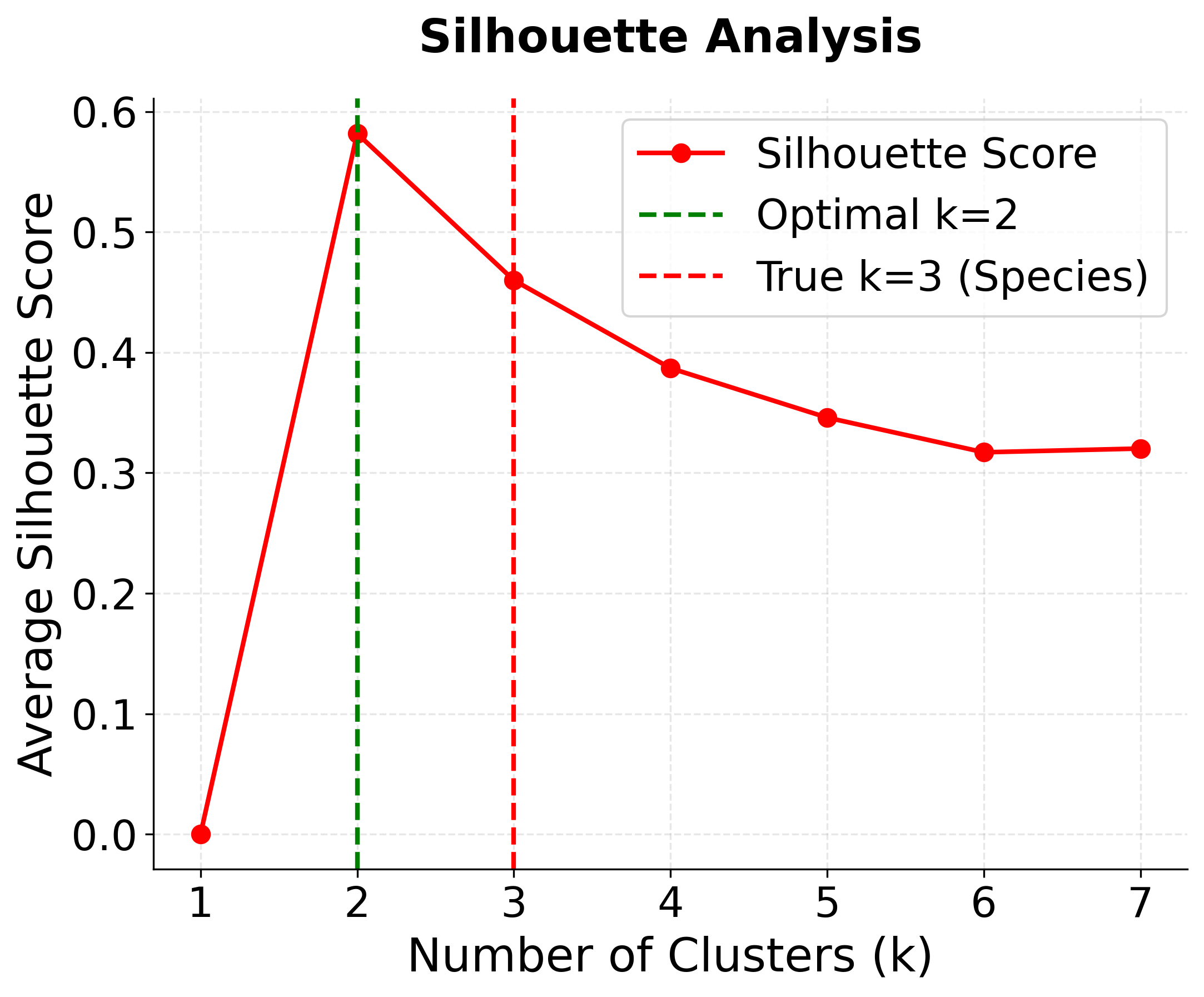
Let's determine the optimal number of clusters for the Iris dataset using both elbow method and silhouette analysis.

This reveals an important insight: the optimal k depends on the evaluation metric:

• Silhouette analysis suggests k=2 (0.681 score) - this groups the more similar Versicolor and Virginica together, which is mathematically optimal but ignores biological reality
• True biological reality is k=3 - three distinct species exist, and k=3 still performs well (0.553 score)
• Domain knowledge matters - sometimes the mathematically optimal solution doesn't align with real-world understanding

Step 8: Final Visualization of Iris Results

Let's visualize the final clustering results on the Iris dataset to see how well K-means performs on real data.

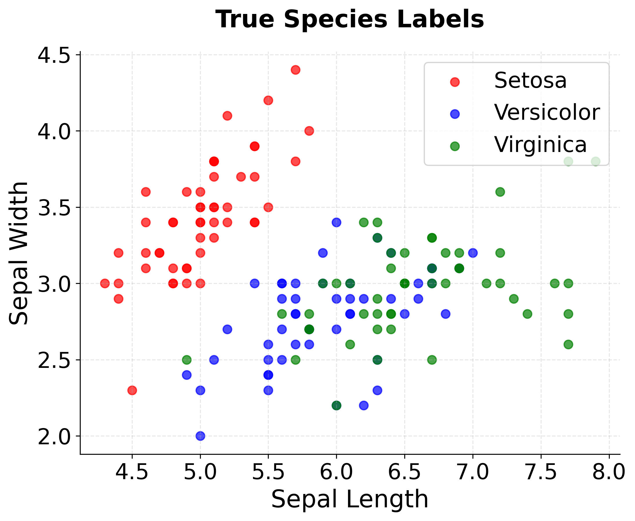
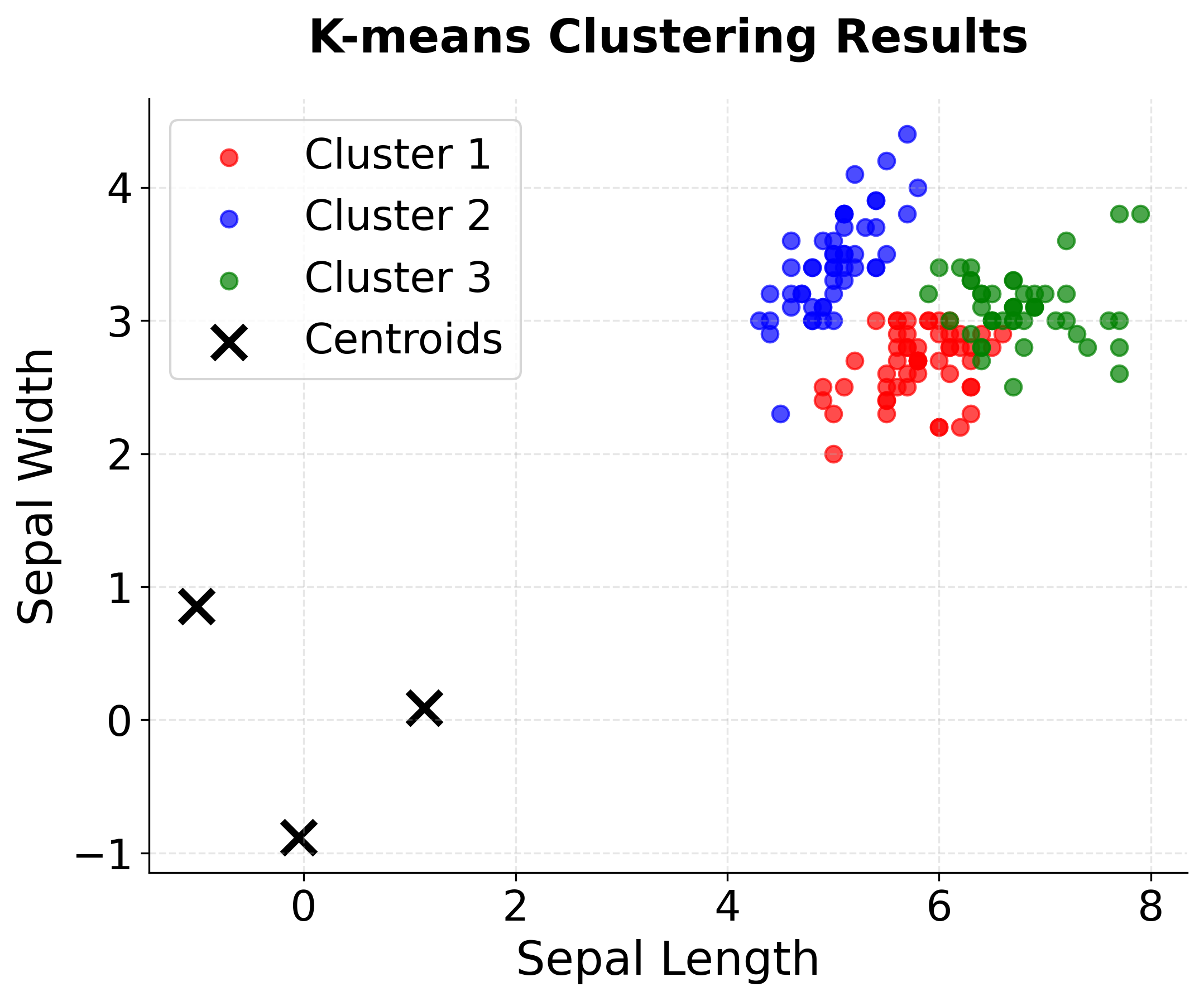
You can see how the visualizations reveal the clustering challenges in real data:

• Setosa is perfectly separated - the algorithm correctly identifies this distinct species
• Versicolor and Virginica show overlap - some misclassification occurs in the boundary region
• Overall good performance - the algorithm captures the main species structure despite natural variation

Key Parameters

Understanding the key parameters and methods is important for effective K-means implementation. Here's a comprehensive guide to the most important aspects:

Parameter Descriptions

• n_clusters: The number of clusters k to form - this is the most important parameter that needs to be specified before running the algorithm
• init: Initialization method ('k-means++' is default and recommended for better convergence than random initialization)
• n_init: Number of times the algorithm runs with different centroid seeds (default 10, higher values reduce risk of poor local optima)
• max_iter: Maximum iterations per run (default 300, usually sufficient for convergence)
• random_state: Seed for reproducible results (important for research, debugging, and consistent results)
• algorithm: The algorithm variant ('lloyd' is the standard K-means, 'elkan' is faster for well-separated clusters)

Best Practices

To achieve the best results with K-means clustering, it is important to follow several best practices. First, standardize your data before applying K-means, as the algorithm is highly sensitive to the scale of features due to its reliance on distance calculations. Using multiple initializations (setting n_init greater than 1) is recommended to avoid poor local optima and to ensure more robust clustering outcomes. When evaluating your clustering results, do not rely solely on inertia, since this metric decreases monotonically as the number of clusters increases. Instead, combine inertia with other evaluation methods such as silhouette analysis for a more comprehensive assessment.

It is also advisable to use the k-means++ initialization method, as it typically leads to better clustering performance compared to random initialization. For reproducibility, set the random_state parameter, which ensures that your results are consistent across different runs. When assessing the quality of your clusters, use multiple metrics (such as the silhouette score, inertia, and your own domain knowledge) to gain a well-rounded understanding of the results. Finally, consider the characteristics of your data: K-means performs best when clusters are roughly spherical and of similar size.

Common Pitfalls

Some common pitfalls can undermine the effectiveness of K-means clustering if not carefully addressed. One frequent mistake is neglecting to standardize the data before clustering. Since K-means relies on distance calculations, features with larger scales can disproportionately influence the results, leading to misleading clusters. Another issue arises when the algorithm is run with only a single initialization; this increases the risk of converging to a poor local optimum, as K-means is sensitive to the initial placement of centroids.

Selecting the number of clusters (k) based solely on inertia is also problematic, as inertia will decrease as more clusters are added, potentially encouraging overfitting. It is important to combine inertia with other evaluation metrics and domain knowledge to make an informed choice. Ignoring domain expertise can result in clusters that are mathematically optimal but do not align with real-world categories or business objectives. Finally, failing to validate clustering results using multiple metrics and visualizations can obscure issues such as poorly separated clusters or misclassifications.

Practical Implications

K-means clustering is particularly valuable in several practical scenarios where data naturally forms spherical, well-separated groups. In customer segmentation, K-means works effectively when customer groups have distinct purchasing behaviors and demographic characteristics that create clear separations in the feature space. The algorithm can identify customer segments such as high-value loyalists, price-sensitive bargain hunters, and occasional browsers, enabling targeted marketing campaigns and personalized recommendations.

The algorithm is also highly effective in image processing applications, particularly for color quantization where the goal is to reduce color complexity while maintaining visual quality. K-means serves as a fundamental technique for clustering pixel colors into representative palettes that reduce storage requirements. This approach is valuable for web applications requiring fast loading times, social media platforms optimizing bandwidth usage, and artistic applications creating stylized effects.

In exploratory data analysis and pattern recognition, K-means provides a foundation for understanding data structure when the underlying clusters are roughly spherical and of similar size. The resulting centroids provide interpretable representatives for each cluster, which can be valuable for understanding the characteristics of different groups in the data. However, the algorithm's effectiveness depends on the data meeting its assumptions about cluster shape and size.

Best Practices

To achieve optimal results with K-means clustering, follow several key practices. First, always standardize your data before applying K-means, as the algorithm is sensitive to feature scales due to its reliance on distance calculations. Use multiple initializations (setting n_init greater than 1) to avoid poor local optima and ensure more robust clustering outcomes. When evaluating clustering results, do not rely solely on inertia, since this metric decreases monotonically as the number of clusters increases. Instead, combine inertia with other evaluation methods such as silhouette analysis for a more comprehensive assessment.

Use the k-means++ initialization method, as it typically leads to better clustering performance compared to random initialization. For reproducibility, always set the random_state parameter to ensure consistent results across different runs. When assessing cluster quality, use multiple metrics (such as the silhouette score, inertia, and domain knowledge) to gain a well-rounded understanding of the results. Consider the characteristics of your data: K-means performs best when clusters are roughly spherical and of similar size.

Data Requirements and Pre-processing

K-means requires numerical data with features that are comparable in scale, making data standardization critical for successful clustering. Since the algorithm uses Euclidean distance calculations, features with larger scales will dominate the clustering process, potentially leading to misleading results. Apply StandardScaler or MinMaxScaler before clustering to ensure all features contribute equally to the distance calculations. The algorithm assumes that all features are equally important, so consider using feature selection techniques or dimensionality reduction methods like PCA if you have many irrelevant or highly correlated features.

The algorithm works best with clean, complete datasets that have minimal missing values and outliers. Missing values should be imputed using appropriate strategies (mean, median, or more sophisticated methods), and outliers should be identified and either removed or handled carefully, as they can significantly affect centroid positions and cluster boundaries. Categorical variables need to be encoded (using one-hot encoding or label encoding) before clustering, and the choice of encoding method can impact results. Ensure your dataset has sufficient data points relative to the number of features to avoid the curse of dimensionality, which can lead to poor clustering performance in high-dimensional spaces.

Common Pitfalls

Several common pitfalls can undermine the effectiveness of K-means clustering. One frequent mistake is neglecting to standardize the data before clustering. Since K-means relies on distance calculations, features with larger scales can disproportionately influence the results, leading to misleading clusters. Another issue arises when the algorithm is run with only a single initialization; this increases the risk of converging to a poor local optimum, as K-means is sensitive to the initial placement of centroids.

Selecting the number of clusters (k) based solely on inertia is also problematic, as inertia will decrease as more clusters are added, potentially encouraging overfitting. It is important to combine inertia with other evaluation metrics and domain knowledge to make an informed choice. Ignoring domain expertise can result in clusters that are mathematically optimal but do not align with real-world categories or business objectives. Finally, failing to validate clustering results using multiple metrics and visualizations can obscure issues such as poorly separated clusters or misclassifications.

Computational Considerations

K-means clustering has a time complexity of O(nkt), where n is the number of data points, k is the number of clusters, and t is the number of iterations until convergence. For large datasets (typically >100,000 points), consider sampling strategies or use Mini-Batch K-means to make the algorithm computationally feasible. The algorithm's memory requirements are generally modest, but for very large datasets, consider using sparse representations or chunking strategies to manage memory usage effectively.

Performance and Deployment Considerations

Evaluating K-means clustering performance requires multiple metrics since no single measure captures all aspects of clustering quality. The inertia (within-cluster sum of squares) provides a baseline measure of cluster compactness but decreases monotonically with increasing k, making it insufficient alone. Combine inertia with silhouette analysis, which measures how well each point fits within its assigned cluster compared to other clusters. For datasets with known ground truth, use external metrics like adjusted rand index or normalized mutual information to validate results. Good clustering results typically show high silhouette scores (>0.5), low inertia relative to the number of clusters, and meaningful separation between cluster centroids.

Deployment considerations for K-means include its scalability to large datasets due to O(nkt) time complexity, where iterations (t) are typically much smaller than data points (n). For very large datasets (millions of points), consider Mini-Batch K-means, which uses random samples for each iteration, significantly reducing computational time while maintaining reasonable quality. The algorithm is well-suited for batch processing and can be easily parallelized for distributed computing environments. In production, monitor clustering stability by tracking centroid positions and cluster assignments over time, and consider retraining the model periodically as new data arrives to maintain relevance and accuracy.

Summary

K-means clustering stands as one of the most fundamental and widely-applied unsupervised learning algorithms in machine learning. Through its elegant iterative process of assigning data points to clusters and updating centroids, K-means successfully partitions datasets into k distinct groups, making it invaluable for exploratory data analysis, customer segmentation, image processing, and pattern recognition across numerous industries.

The algorithm's mathematical foundation centers on minimizing the within-cluster sum of squares, which translates to finding compact, well-separated clusters. While K-means excels with spherical, similarly-sized clusters, it has important limitations including sensitivity to initialization, the need to specify k beforehand, and assumptions about cluster shape that may not hold for all real-world datasets. These limitations underscore the importance of proper data preprocessing, careful parameter selection, and thorough evaluation using multiple quality metrics.

The practical implementation of K-means requires attention to data standardization, appropriate initialization strategies, and robust evaluation methods. When applied correctly with suitable data characteristics, K-means provides interpretable, efficient clustering solutions that serve as excellent baselines and stepping stones to more sophisticated clustering techniques. The algorithm's computational efficiency and conceptual simplicity make it an essential tool in the data scientist's toolkit, particularly valuable for initial data exploration and when computational resources are constrained.

Quiz

Ready to test your understanding? Take this quick quiz to reinforce what you've learned about K-means clustering.