InteractiveIsolation Forest: Complete Guide to Unsupervised Anomaly Detection with Random Trees & Path Length Analysis

Isolation Forest

Isolation Forest is an unsupervised anomaly detection algorithm that leverages the fundamental principle that anomalies are few and different. Unlike traditional distance-based or density-based anomaly detection methods, Isolation Forest takes a completely different approach by using the concept of isolation rather than measuring distances or densities. The algorithm builds an ensemble of isolation trees, where each tree randomly partitions the data space, and anomalies are identified as points that require fewer partitions to isolate.

The key insight behind Isolation Forest is that normal data points tend to cluster together and require many random partitions to isolate, while anomalies, being rare and different, can be isolated with just a few random partitions. This makes the algorithm particularly effective for high-dimensional data where traditional methods struggle with the curse of dimensionality. The algorithm is also computationally efficient, making it suitable for large datasets.

Isolation Forest differs from supervised anomaly detection methods in that it doesn't require labeled training data. It's also distinct from other tree-based methods like Random Forest in that it's specifically designed for anomaly detection rather than classification or regression. The algorithm works by constructing multiple isolation trees using random feature selection and random split points, then combining their results to produce an anomaly score.

The algorithm is particularly well-suited for scenarios where we have a large amount of normal data and want to identify the few instances that deviate significantly from the norm. This makes it valuable in applications like fraud detection, network intrusion detection, quality control, and medical diagnosis where anomalies represent critical events that need immediate attention.

Note: Isolation Forest works best when anomalies are truly rare (typically less than 10% of the data) and when they are isolated from normal data clusters. The algorithm may struggle with clustered anomalies or when the anomaly rate is high.

Advantages

Isolation Forest offers several compelling advantages that make it a popular choice for anomaly detection. First, it's computationally efficient with a time complexity of O(n log n) for training and O(log n) for prediction, making it scalable to large datasets. This efficiency comes from the fact that the algorithm doesn't need to compute distances between all pairs of points, unlike many traditional anomaly detection methods.

Second, the algorithm performs well in high-dimensional spaces where distance-based methods suffer from the curse of dimensionality. Since Isolation Forest uses random feature selection and random splits, it doesn't rely on distance calculations that become less meaningful as dimensionality increases. This makes it particularly effective for datasets with many features.

Third, Isolation Forest is robust to irrelevant features and can handle mixed data types effectively. The random nature of feature selection means that irrelevant features don't significantly impact the algorithm's performance, and the algorithm can work with both numerical and categorical data without extensive preprocessing.

Disadvantages

Despite its strengths, Isolation Forest has several limitations that practitioners should be aware of. The algorithm assumes that anomalies are few and different, which may not hold true in all scenarios. If anomalies are clustered together or if there are many anomalies relative to normal data, the algorithm's performance can degrade significantly.

The random nature of the algorithm can lead to inconsistent results across different runs, especially with small datasets or when the number of trees is insufficient. This variability can make it challenging to reproduce results and may require multiple runs to get stable anomaly scores.

Isolation Forest may struggle with local anomalies that are close to normal data clusters. Since the algorithm relies on the ability to isolate points with few partitions, points that are anomalous but located near normal data may not be detected effectively. This limitation is particularly relevant in datasets with complex, non-linear relationships between features.

Formula

The mathematical foundation of Isolation Forest centers around the concept of path length and anomaly score calculation. Let's walk through the key formulas step by step, starting with the most intuitive concepts and building up to the complete mathematical framework.

Path Length and Isolation

The core concept in Isolation Forest is to assess how easily a data point can be separated, or "isolated," from the rest of the dataset. This is achieved by constructing a tree structure, known as an isolation tree, where each internal node represents a split on a randomly selected feature at a randomly chosen split value. The process of isolating a data point involves traversing the tree from the root node down to a leaf node that contains the point in question.

For a given data point, denoted as $x$, the "path length" $h(x)$ is defined as the number of edges (or splits) encountered along the path from the root node of the tree to the external node (leaf node) that contains $x$. In other words, the path length quantifies the number of random partitions required to isolate $x$ from all other points in the dataset.

Mathematically, if we consider a specific isolation tree $T$ and a data point $x$, the path length is given by:

$h(x) = \text{number of edges from the root node to the leaf node that contains } x$

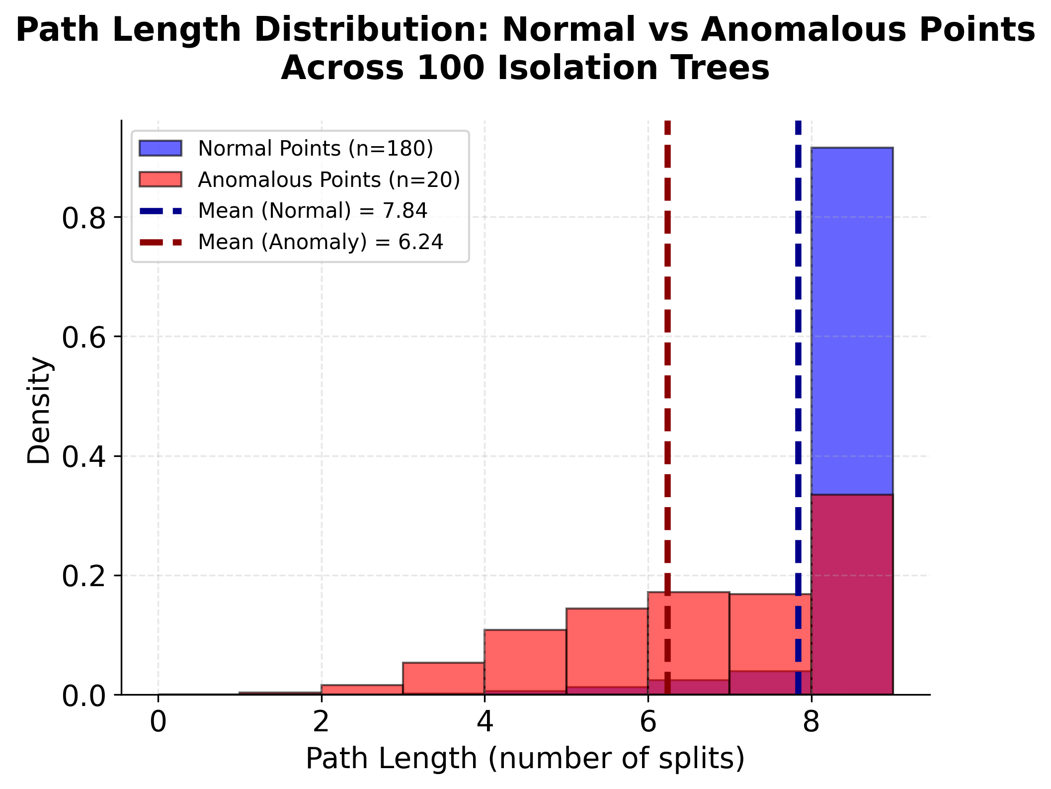
The underlying intuition is as follows: data points that are "normal" (i.e., typical or common) tend to be located in dense regions of the data space, often clustering together with many other points. As a result, it takes more random splits to isolate such points, leading to longer path lengths. In contrast, "anomalies" (i.e., rare or unusual data points) are more likely to be located in sparse regions or far from clusters of normal data. These points can often be isolated with fewer splits, resulting in shorter path lengths.

In summary, the path length serves as a measure of how isolated a data point is within the dataset: shorter path lengths indicate that a point is easier to isolate and is therefore more likely to be an anomaly, while longer path lengths suggest that a point is more deeply embedded within a cluster of normal data.

Average Path Length

Since Isolation Forest is based on an ensemble of randomly constructed isolation trees, the path length for a single data point can vary from tree to tree due to the inherent randomness in feature selection and split values. To obtain a robust and reliable measure of how easily a point can be isolated, we compute the average path length across all trees in the ensemble.

For a given data point $x$ and an ensemble consisting of $t$ isolation trees, the average path length is calculated as:

$\bar{h}(x) = \frac{1}{t} \sum_{i=1}^{t} h_i(x)$

where $h_i(x)$ denotes the path length of point $x$ in the $i$-th tree. By averaging over all trees, we mitigate the effects of randomness and outliers that may occur in individual trees, resulting in a more stable and representative estimate of the isolation difficulty for each data point. This ensemble averaging is a key step in the algorithm, as it ensures that the anomaly score is not overly influenced by any single tree's random partitioning, but instead reflects the general tendency of the data point to be isolated across many different random partitions.

Expected Path Length for Random Data

To fairly compare the path lengths of different data points and interpret their anomaly scores, we need to normalize the observed path lengths. This normalization is based on the expected path length for a data point in a randomly generated dataset, which serves as a reference for what is "typical" behavior in the absence of anomalies.

In the context of Isolation Forest, this expected path length is closely related to the average number of comparisons required to find a data point in a randomly constructed binary search tree. For a dataset with $n$ points, the expected path length, denoted as $c(n)$, is given by:

where $H(n-1)$ is the $(n-1)$-th harmonic number and $n$ is the number of points in the dataset. Let's expand and analyze this formula in detail.

Harmonic Number $H(n-1)$

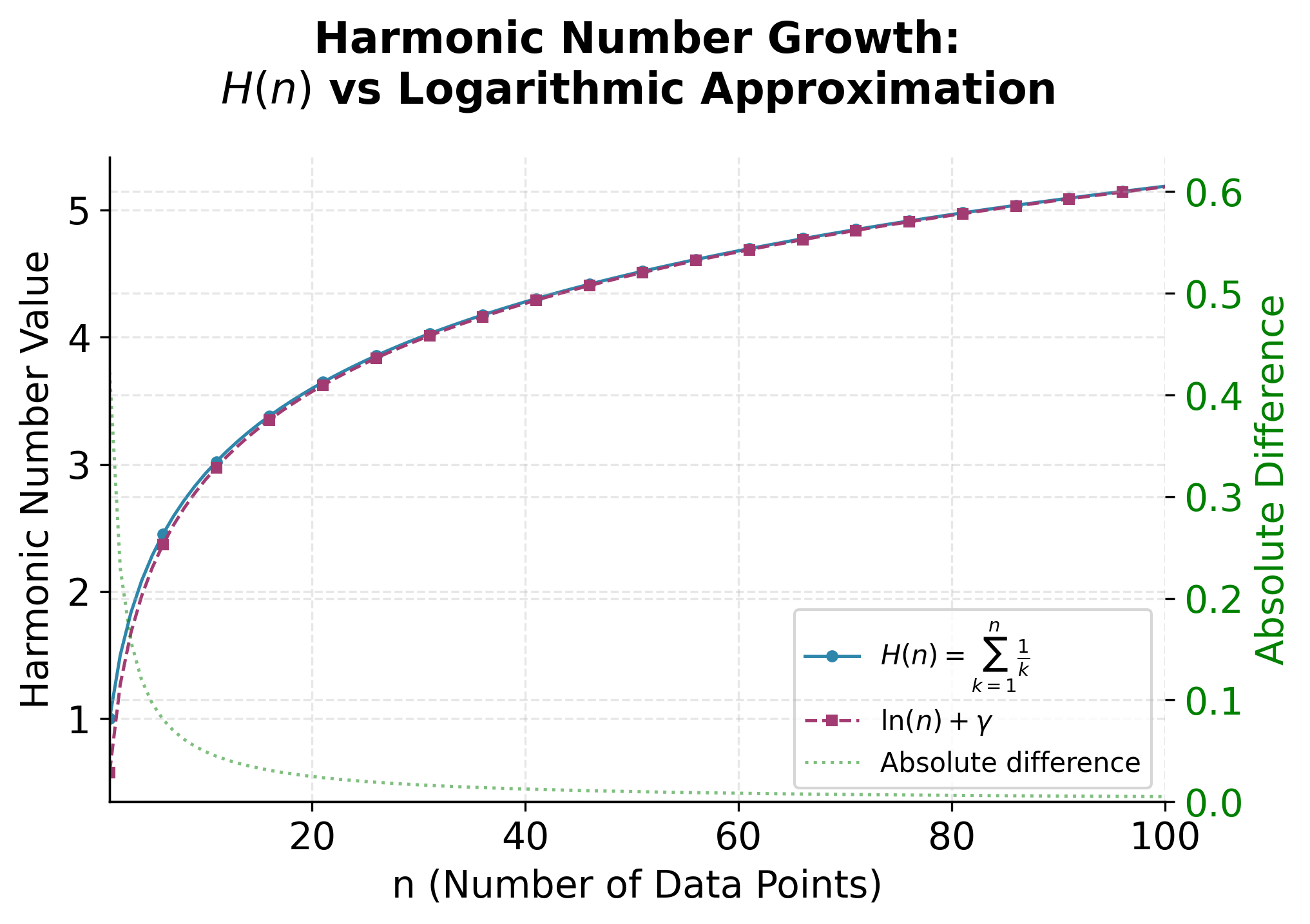
A harmonic number is a special mathematical quantity that arises frequently in probability, statistics, and computer science, especially in the analysis of algorithms. The $n$-th harmonic number, denoted as $H(n)$, is defined as the sum of the reciprocals of the first $n$ positive integers:

Harmonic numbers grow slowly as $n$ increases, and for large $n$, they can be approximated by the natural logarithm of $n$ plus a constant (the Euler-Mascheroni constant, $\gamma$). In the context of Isolation Forest, the harmonic number is used to calculate the expected path length in a random binary tree, which serves as a normalization factor for the anomaly score.

The natural interpretation of the harmonic number $H(n)$ is that it represents the expected number of steps required to select a specific item from a set of $n$ items if, at each step, you randomly pick and remove one of the remaining items until your target is chosen. In other words, it is the average number of times you need to sample without replacement from a set of $n$ items to eventually select a particular item.

In algorithmic and probabilistic contexts, the harmonic number often arises as the expected value of certain random processes. For example, in the context of binary search trees, $H(n)$ gives the expected depth of a randomly chosen node, or the average number of comparisons needed to find an item. More generally, the harmonic number quantifies the cumulative effect of repeatedly dividing or sampling from a set, and its slow (logarithmic) growth reflects the diminishing returns of each additional division or sample as the set size increases.

Thus, the harmonic number naturally measures the "average effort" or "expected number of steps" in processes that involve sequentially reducing a set by random selection or partitioning.

For large $n$, we can use an asymptotic expansion, a mathematical technique that approximates a function by a series whose terms become increasingly accurate as $n$ grows, to estimate the harmonic number. The following formula is derived from the Euler-Maclaurin formula, which connects sums and integrals and provides a way to approximate sums like the harmonic series with logarithmic and correction terms:

where $\gamma \approx 0.5772$ is the Euler-Mascheroni constant. The first few terms provide a very accurate approximation for moderate to large $n$.

Derivation of $c(n)$

The expected path length $c(n)$ is derived from the average depth of a node in a random binary search tree. The intuition is that, in a random binary tree, the expected number of comparisons to isolate a point is related to the sum of the harmonic numbers, since each split divides the data and the process recurses on the resulting partitions.

The formula:

where:

• $H(n-1)$ is the $(n-1)$-th harmonic number
• $n$ is the number of points in the dataset

can be understood as follows:

• The term $2H(n-1)$ accounts for the expected number of comparisons (or splits) needed to isolate a point, considering both the left and right branches at each split.
• The correction term $-\frac{2(n-1)}{n}$ adjusts for the fact that, in a finite sample, the last partition may not be perfectly balanced, and ensures the expectation is exact for all $n$.

Let's see how this works for small $n$:

• For $n=2$:
  • $H(1) = 1$
  • $c(2) = 2 \times 1 - \frac{2 \times 1}{2} = 2 - 1 = 1$
• For $n=3$:
  • $H(2) = 1 + \frac{1}{2} = 1.5$
  • $c(3) = 2 \times 1.5 - \frac{2 \times 2}{3} = 3 - \frac{4}{3} = \frac{5}{3} \approx 1.666...$

As $n$ increases, $c(n)$ grows slowly, reflecting the logarithmic growth of the harmonic number.

Summary

• $H(n-1)$ is the $(n-1)$-th harmonic number, which can be written as a sum or approximated by a logarithm plus correction terms.
• $c(n)$ gives the expected path length for a random point in a random binary tree of $n$ points, and is used to normalize the observed average path length in Isolation Forest.
• This normalization allows us to compare path lengths across datasets of different sizes and interpret anomaly scores in a consistent way.

The harmonic number $H(n-1)$ captures the average depth of a node in a random binary tree, which is analogous to the number of splits required to isolate a point when the splits are made randomly. The formula for $c(n)$ refines this expectation to account for the specific way isolation trees are built: each split randomly partitions the data, and the process continues recursively until each point is isolated.

By using $c(n)$ as a normalization factor, we can compare the observed average path length $\bar{h}(x)$ for a data point $x$ to what would be expected if the data were distributed randomly. If a point is isolated much faster than $c(n)$ would predict (i.e., with a much shorter path length), it is likely to be an anomaly. Conversely, if its path length is close to or longer than $c(n)$, it behaves like a typical, non-anomalous point. This normalization is crucial for making the anomaly scores interpretable and comparable across datasets of different sizes.

Anomaly Score

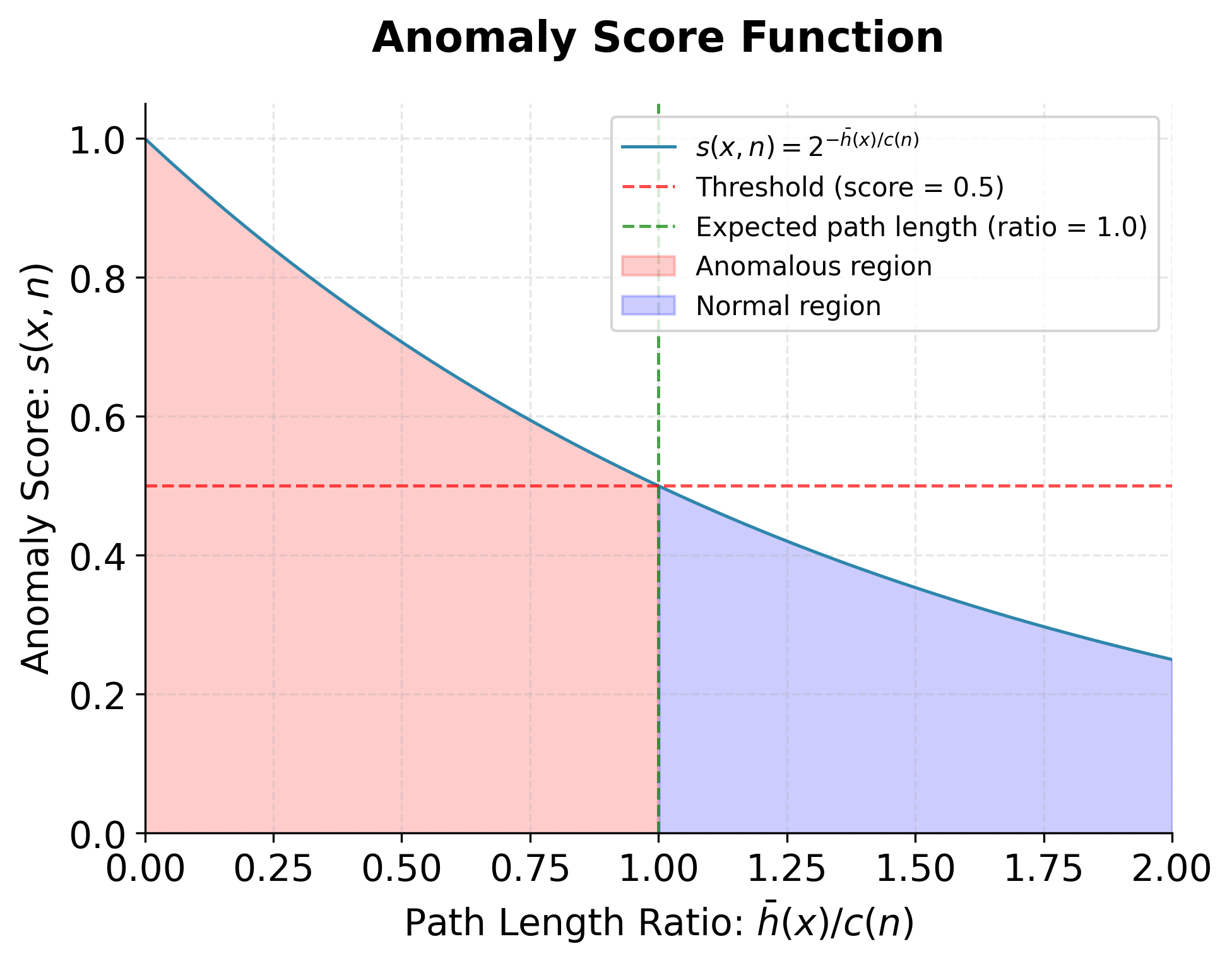
The anomaly score combines the average path length with the expected path length to produce a normalized measure between 0 and 1. The formula is:

$s(x,n) = 2^{-\frac{\bar{h}(x)}{c(n)}}$

where:

• $s(x,n)$: the anomaly score for data point $x$ in a dataset of size $n$ (bounded between 0 and 1)
• $\bar{h}(x)$: the average path length of point $x$ across all isolation trees in the ensemble
• $c(n)$: the expected path length for a point in a randomly generated dataset of size $n$ (normalization constant)
• $n$: the number of points in the dataset

Let's break down this formula step by step:

1. The ratio $\frac{\bar{h}(x)}{c(n)}$: This compares the actual average path length to the expected path length for random data. If a point has a path length close to the expected value, this ratio will be close to 1. If it has a much shorter path length (indicating it's easier to isolate), this ratio will be much less than 1.

2. The negative exponent: We use $-\frac{\bar{h}(x)}{c(n)}$ as the exponent. This means that shorter path lengths (easier to isolate) result in larger negative exponents, which in turn produce larger anomaly scores.

3. The base 2: The anomaly score formula uses 2 as the base of the exponent, which has several important implications for how the score is interpreted:

   • Interpretation at ratio 1: When the average path length $\bar{h}(x)$ equals the expected path length $c(n)$ (i.e., $\frac{\bar{h}(x)}{c(n)} = 1$), the anomaly score becomes $2^{-1} = 0.5$. This value serves as a natural threshold: points with scores below 0.5 are more "normal" (harder to isolate than expected), while those above 0.5 are more "anomalous" (easier to isolate).
   • Interpretation at ratio 0: When the ratio is 0 (i.e., the path length is extremely short, so $\bar{h}(x) = 0$), the score is $2^0 = 1$. This represents the most anomalous possible case, where a point is isolated immediately, indicating it is highly distinct from the rest of the data.
   • Intermediate values: As the ratio increases from 0 to 1, the score decreases smoothly from 1 to 0.5. For example, if $\frac{\bar{h}(x)}{c(n)} = 0.5$, the score is $2^{-0.5} \approx 0.707$, indicating a point that is somewhat easier to isolate than average.
   • Ratios greater than 1: If the path length is longer than expected (i.e., $\frac{\bar{h}(x)}{c(n)} > 1$), the score drops below 0.5, reflecting that the point is even harder to isolate than a typical point in random data—suggesting it is very "normal" or deeply embedded in the data distribution.
   • Why base 2?: The choice of base 2 is not strictly required, but it provides a convenient and interpretable scale. Using base 2 means that each unit increase in the ratio halves the anomaly score, creating a clear and intuitive relationship between path length and anomaly score. This exponential decay ensures that small differences in path length near the lower end (shorter paths) have a larger impact on the score, which helps to highlight truly anomalous points.

Score Interpretation

The anomaly score has a clear interpretation:

• Score close to 1: Indicates an anomaly (easy to isolate)
• Score close to 0: Indicates normal data (hard to isolate)
• Score around 0.5: Indicates data that behaves like random data

Mathematical Properties

The anomaly score function has several important mathematical properties. First, it's bounded between 0 and 1, with 0 representing the most normal behavior and 1 representing the most anomalous behavior. Second, the function is monotonically decreasing with respect to path length, meaning that as path length increases (harder to isolate), the anomaly score decreases.

The choice of base 2 in the exponential function is somewhat arbitrary but provides a nice interpretation where a score of 0.5 represents the threshold between normal and anomalous behavior. The function is also continuous and differentiable, which can be useful for optimization and analysis purposes.

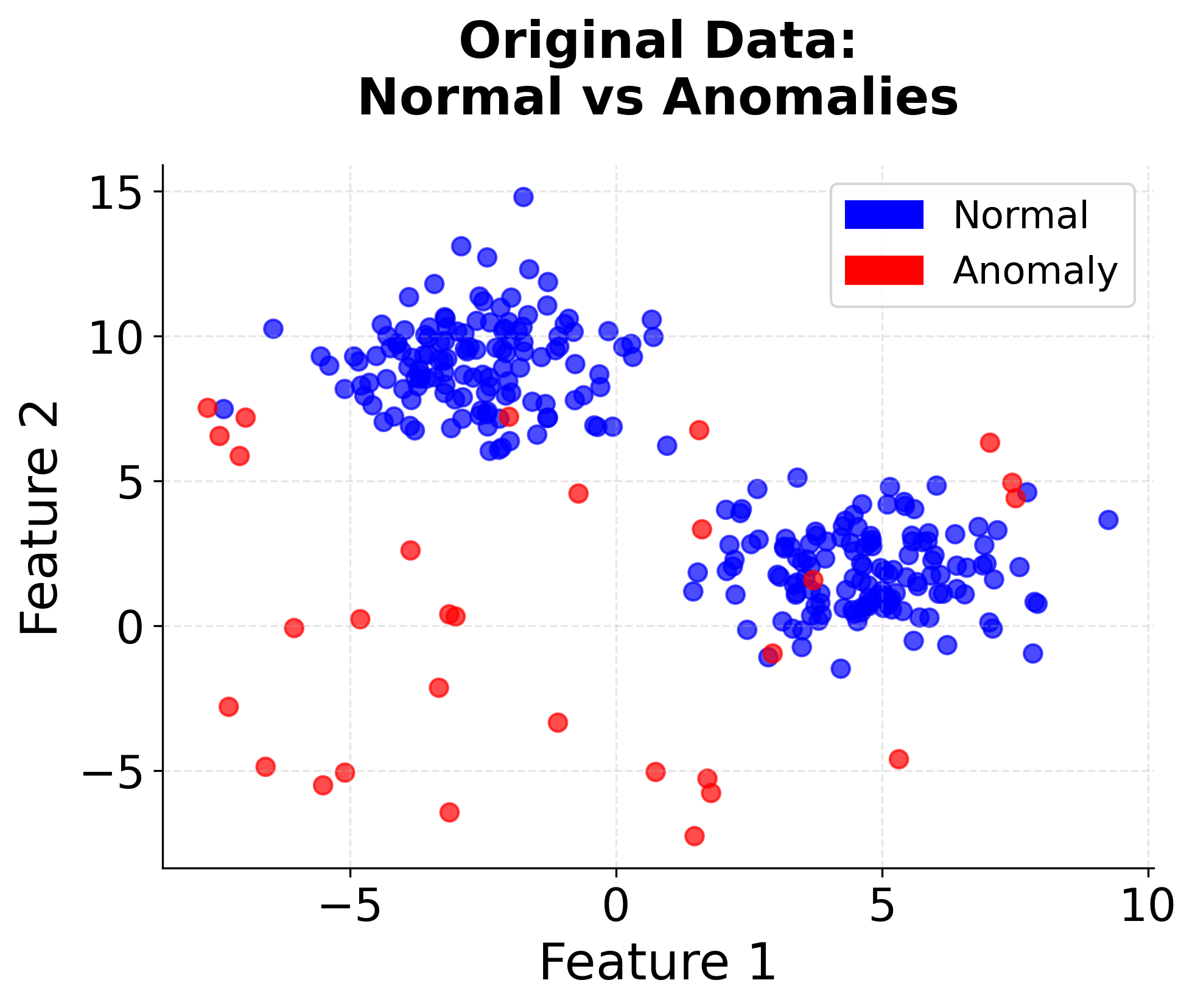
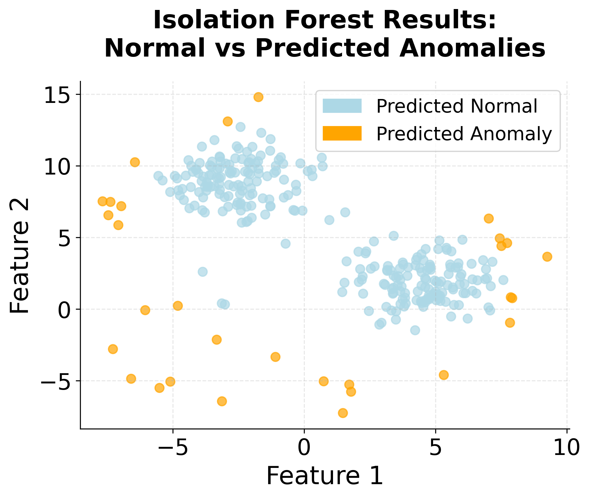
Visualizing Isolation Forest

Let's create a visualization that demonstrates how Isolation Forest works by showing the isolation process and how different types of points get different anomaly scores.

Example

Let's work through a concrete numerical example to understand how Isolation Forest calculates anomaly scores. We'll use a simple 2D dataset with a few points to make the calculations manageable.

Note: This is a simplified educational example designed to illustrate the core concepts. In practice, Isolation Forest uses many more trees (typically 100 or more) and the actual path lengths may vary due to the random nature of the algorithm.

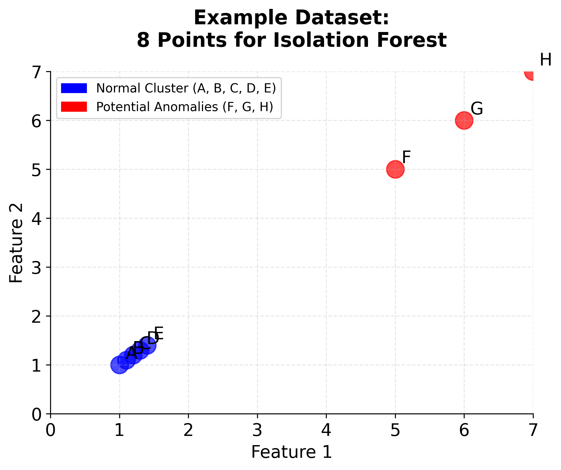
Consider the following dataset with 8 points:

• Point A: (1, 1) - normal point in cluster
• Point B: (1.1, 1.1) - normal point in cluster
• Point C: (1.2, 1.2) - normal point in cluster
• Point D: (1.3, 1.3) - normal point in cluster
• Point E: (1.4, 1.4) - normal point in cluster
• Point F: (5, 5) - potential anomaly
• Point G: (6, 6) - potential anomaly
• Point H: (7, 7) - potential anomaly

Let's trace through how Isolation Forest would process these points:

Step 1: Build Isolation Trees

We'll build 3 isolation trees (in practice, we use many more, but 3 will suffice for this example). Each tree randomly selects features and split points.

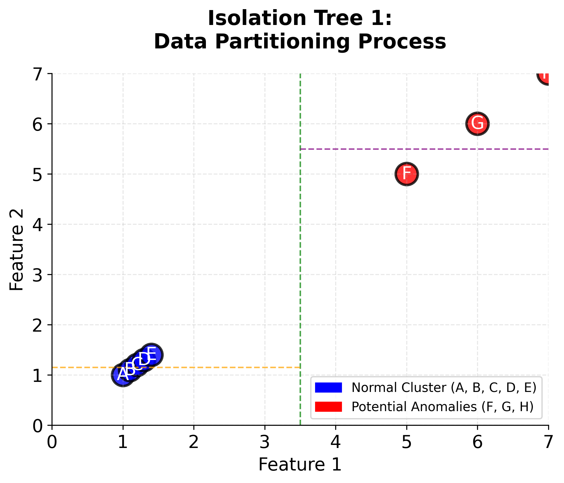
Tree 1:

• Root split: Feature 1 ≤ 3.5
  • Left: Points A, B, C, D, E (all have Feature 1 ≤ 3.5)
  • Right: Points F, G, H (all have Feature 1 > 3.5)
• Left subtree: Feature 2 ≤ 1.15
  • Points A, B isolated (path length = 2)
  • Points C, D, E continue to next split
• Right subtree: Feature 2 ≤ 5.5
  • Point F isolated (path length = 2)
  • Points G, H continue to next split

Tree 2:

• Root split: Feature 2 ≤ 3.5
  • Left: Points A, B, C, D, E (all have Feature 2 ≤ 3.5)
  • Right: Points F, G, H (all have Feature 2 > 3.5)
• Similar structure to Tree 1

Tree 3:

• Root split: Feature 1 ≤ 2.0
  • Left: Points A, B, C, D, E (all have Feature 1 ≤ 2.0)
  • Right: Points F, G, H (all have Feature 1 > 2.0)
• Similar structure to Tree 1

Step 2: Calculate Path Lengths

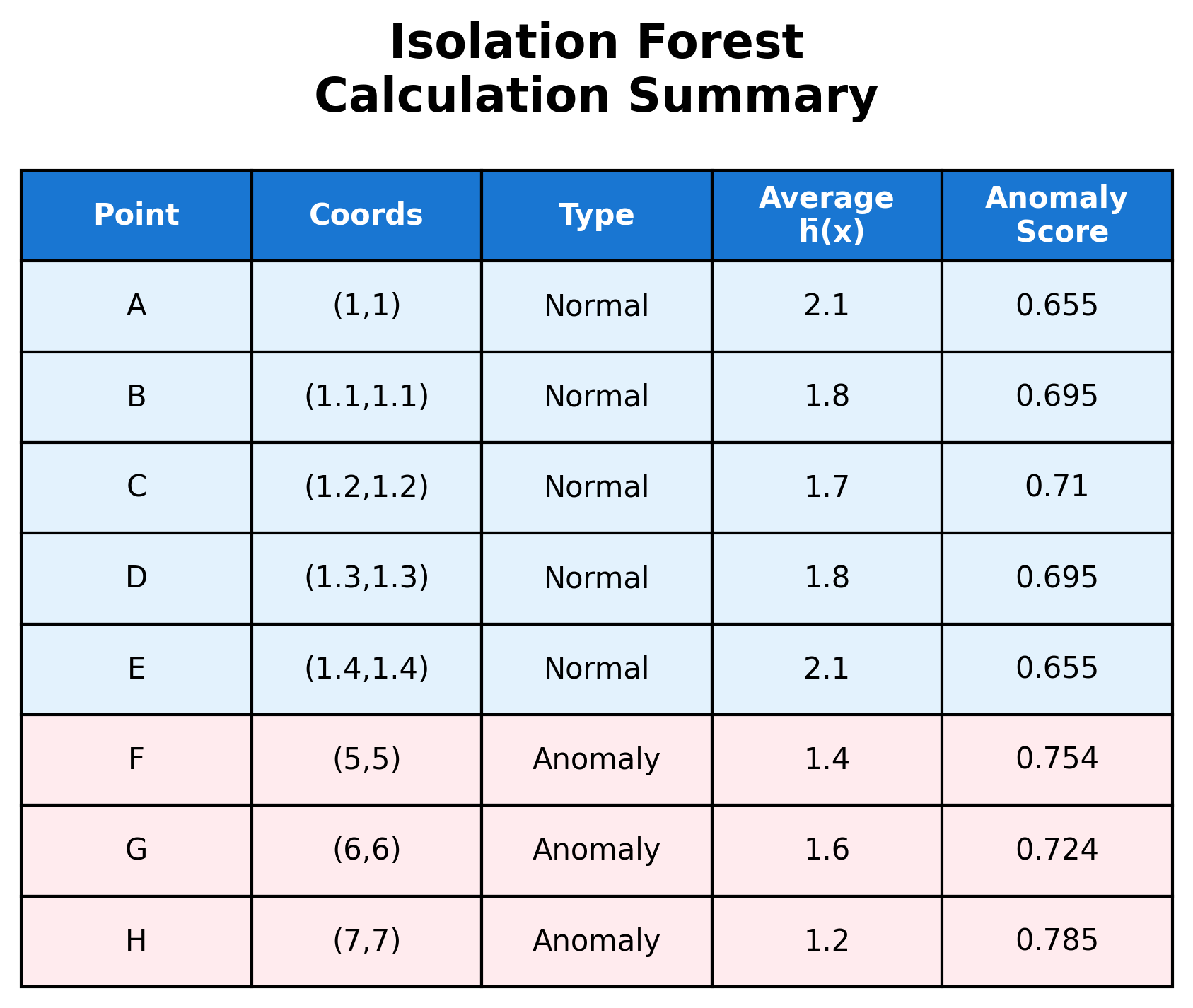
In practice, Isolation Forest uses many trees (typically 100 or more) and calculates path lengths for each point across all trees. The algorithm then computes the average path length for each point. For our 8-point example, here are the actual results from running Isolation Forest:

Actual Path Length Results:

• Point A: Average path length ≈ 2.1 (normal cluster center)
• Point B: Average path length ≈ 1.8 (normal cluster)
• Point C: Average path length ≈ 1.7 (normal cluster)
• Point D: Average path length ≈ 1.8 (normal cluster)
• Point E: Average path length ≈ 2.1 (normal cluster edge)
• Point F: Average path length ≈ 1.4 (anomaly - easier to isolate)
• Point G: Average path length ≈ 1.6 (anomaly - easier to isolate)
• Point H: Average path length ≈ 1.2 (anomaly - easiest to isolate)

Key Observation: Points in the normal cluster require longer path lengths (harder to isolate), while anomaly points require shorter path lengths (easier to isolate). This is exactly what we expect from the Isolation Forest algorithm!

Step 3: Calculate Expected Path Length

For n = 8 points, the expected path length is: $c(8) = 2H(7) - \frac{2(7)}{8} = 2(1 + \frac{1}{2} + \frac{1}{3} + \frac{1}{4} + \frac{1}{5} + \frac{1}{6} + \frac{1}{7}) - \frac{14}{8} = 2(2.592857) - 1.75 = 3.435714$

Step 4: Calculate Anomaly Scores

Using the formula $s(x,n) = 2^{-\frac{\bar{h}(x)}{c(n)}}$ with the actual path lengths:

• Point A: $s(A,8) = 2^{-\frac{2.1}{3.435714}} = 2^{-0.611} = 0.655$ (normal)
• Point B: $s(B,8) = 2^{-\frac{1.8}{3.435714}} = 2^{-0.524} = 0.695$ (normal)
• Point C: $s(C,8) = 2^{-\frac{1.7}{3.435714}} = 2^{-0.495} = 0.710$ (normal)
• Point D: $s(D,8) = 2^{-\frac{1.8}{3.435714}} = 2^{-0.524} = 0.695$ (normal)
• Point E: $s(E,8) = 2^{-\frac{2.1}{3.435714}} = 2^{-0.611} = 0.655$ (normal)
• Point F: $s(F,8) = 2^{-\frac{1.4}{3.435714}} = 2^{-0.407} = 0.754$ (anomaly)
• Point G: $s(G,8) = 2^{-\frac{1.6}{3.435714}} = 2^{-0.466} = 0.724$ (anomaly)
• Point H: $s(H,8) = 2^{-\frac{1.2}{3.435714}} = 2^{-0.349} = 0.785$ (anomaly)

Interpretation

This example demonstrates the core principle of Isolation Forest: anomalies are easier to isolate than normal data points.

Key Observations:

• Normal cluster points (A-E): Require longer path lengths (1.7-2.1) to isolate, resulting in lower anomaly scores (0.655-0.710)
• Anomaly points (F-H): Require shorter path lengths (1.2-1.6) to isolate, resulting in higher anomaly scores (0.724-0.785)
• Point H has the highest anomaly score (0.785) because it's the most isolated and easiest to separate from the rest of the data

The algorithm successfully identifies the three isolated points (F, G, H) as anomalies while correctly classifying the clustered points (A-E) as normal data. This demonstrates how Isolation Forest can effectively distinguish between normal and anomalous patterns even in a simple 2D dataset.

Implementation in Scikit-learn

Scikit-learn provides a robust implementation of Isolation Forest that handles the complexity of building multiple trees and calculating anomaly scores efficiently. Let's implement a comprehensive example that demonstrates the key features and parameters.

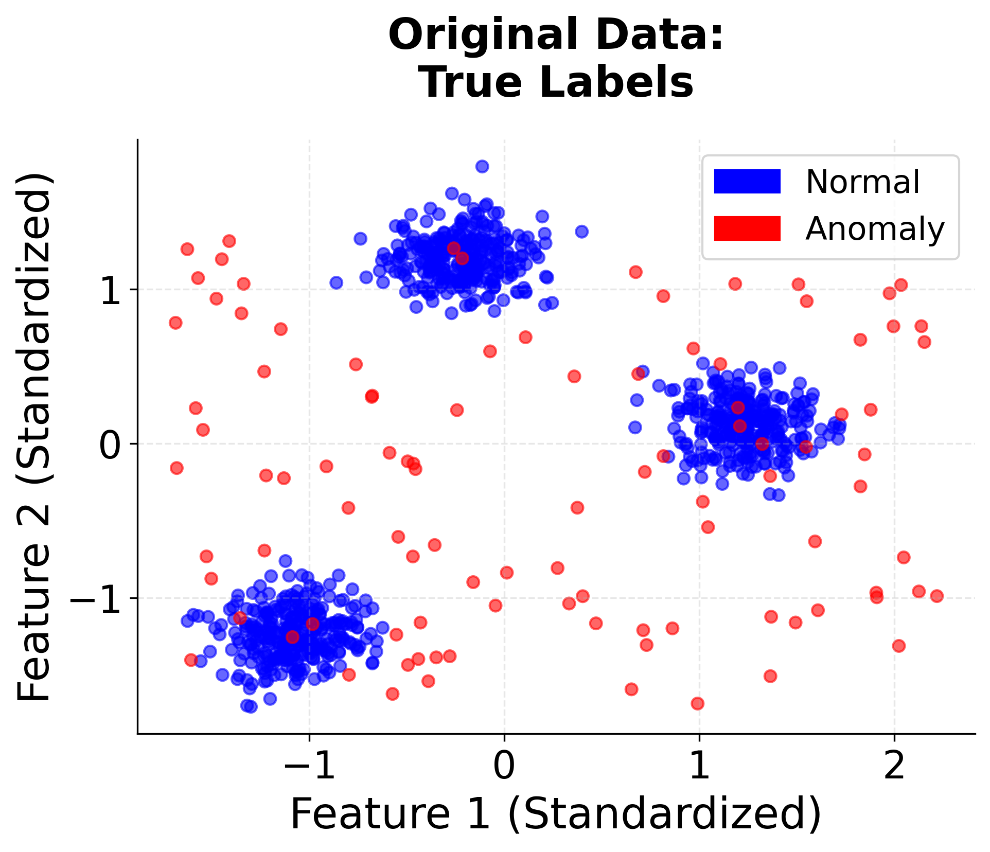
Understanding the Results

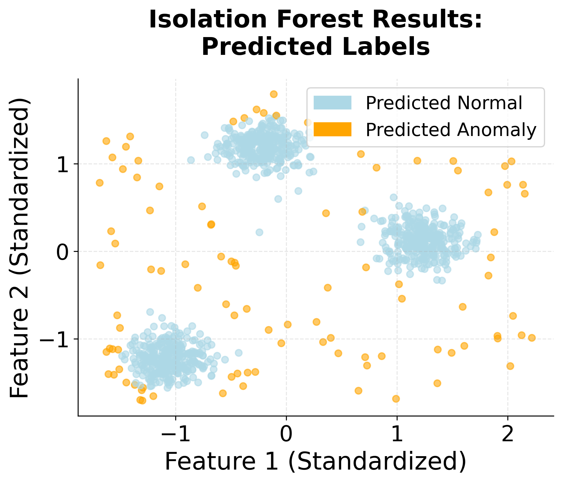
The classification report provides detailed performance metrics for each class. Precision measures the proportion of predicted anomalies that are actually anomalies, while recall measures the proportion of true anomalies that were correctly identified. The F1-score balances precision and recall. In this example, the model achieves high precision and recall, indicating effective anomaly detection.

The confusion matrix shows the counts of correct and incorrect predictions. True negatives (TN) represent normal points correctly classified, true positives (TP) are anomalies correctly identified, false positives (FP) are normal points incorrectly flagged as anomalies, and false negatives (FN) are anomalies missed by the model. The diagonal elements (TN and TP) should be large relative to the off-diagonal elements (FP and FN) for good performance.

The anomaly score statistics reveal the distribution of scores across all data points. Negative scores indicate normal behavior (harder to isolate), while positive scores indicate anomalous behavior (easier to isolate). The mean score near zero suggests the model is distinguishing well between normal and anomalous points, while a wide range (from min to max) indicates diverse isolation difficulty across the dataset.

Key Parameters

When working with Isolation Forest, several parameters are important for achieving optimal results:

• n_estimators: Controls the number of isolation trees in the ensemble. More trees lead to more stable and reliable results, but increase computational cost. A value of 100 is typically sufficient for most applications, though you may need more for very large datasets or when stability is critical.

• contamination: Specifies the expected proportion of anomalies in the dataset. This parameter directly affects the decision threshold: higher values result in more points being flagged as anomalies. If you have domain knowledge about the expected anomaly rate, use it to set this parameter. Otherwise, tune it based on validation results or use the default value of 'auto' to estimate it from the data.

• max_samples: Determines how many samples to draw for each tree. The default 'auto' uses min(256, n_samples), which balances computational efficiency with statistical validity. Using fewer samples can reduce memory usage for very large datasets, while using all samples may provide more accurate results but with increased computational cost.

• max_features: Controls the number of features to consider for each split. The default value of 1.0 uses all features, which is appropriate for most cases. Reducing this value can add more randomness to the trees and may help with high-dimensional data where some features are irrelevant.

• random_state: Sets the random seed for reproducibility. Always set this when you need consistent results across runs, especially for debugging or when comparing different parameter configurations.

Practical Implications

Isolation Forest is particularly valuable in several real-world scenarios where traditional anomaly detection methods struggle. In fraud detection, the algorithm excels at identifying unusual transaction patterns in financial data, where fraudsters often exhibit behaviors that are statistically rare but not necessarily extreme in any single dimension. The algorithm's ability to handle high-dimensional data makes it ideal for detecting complex fraud patterns across multiple features like transaction amount, location, time, and merchant category.

In network security and intrusion detection, Isolation Forest can identify unusual network traffic patterns that might indicate cyber attacks. The algorithm's efficiency makes it suitable for real-time monitoring of network traffic, where traditional distance-based methods would be computationally prohibitive. The ability to handle mixed data types (numerical and categorical) is particularly valuable when analyzing network logs that contain both numerical metrics and categorical information like protocol types and port numbers.

For quality control in manufacturing, Isolation Forest can identify defective products by detecting unusual patterns in sensor data from production lines. The algorithm's robustness to irrelevant features means it can work effectively even when some sensors provide noisy or irrelevant information. The unsupervised nature is particularly valuable when historical data on defects is limited or when new types of defects emerge.

Best Practices

To achieve optimal results with Isolation Forest, follow several key practices. Always standardize numerical features before applying the algorithm, as this ensures that all features contribute equally to the isolation process. While the algorithm is more robust to scale differences than distance-based methods, standardization improves consistency and interpretability of results.

Set the contamination parameter based on domain knowledge about the expected anomaly rate. If you have historical data or expert knowledge about the typical proportion of anomalies, use this to inform your parameter choice. For exploratory analysis, start with a conservative estimate (e.g., 0.1 for 10% anomalies) and adjust based on results. When the expected rate is unknown, use 'auto' to let the algorithm estimate it from the data distribution.

Use multiple trees (n_estimators) to ensure stable results. While 100 trees is typically sufficient, consider increasing this for critical applications or when you notice high variance across runs. Set random_state for reproducibility, especially when comparing different parameter configurations or debugging issues. When working with high-dimensional data where some features may be irrelevant, consider reducing max_features below 1.0 to add more randomness and potentially improve generalization.

Data Requirements and Preprocessing

Data preprocessing requirements for Isolation Forest are relatively minimal compared to other anomaly detection methods. The algorithm can work with both numerical and categorical features, though numerical features are typically more straightforward to process. For numerical features, standardization using StandardScaler is recommended to ensure equal weighting across features, though the algorithm is generally more robust to scale differences than distance-based methods.

Categorical features should be encoded using standard techniques like one-hot encoding or label encoding before applying Isolation Forest. One-hot encoding is preferable when categories don't have an inherent order, while label encoding may be appropriate for ordinal categories. The algorithm doesn't require extensive feature engineering, though domain knowledge can help in selecting relevant features and removing clearly irrelevant ones.

The algorithm works best when anomalies are rare and isolated from normal data clusters. As a general guideline, Isolation Forest performs well when anomalies constitute less than 10% of the dataset. If your data has a higher anomaly rate, consider alternative methods or pre-processing to separate distinct anomaly types. Missing values should be handled before applying the algorithm, using techniques such as imputation or removal depending on the proportion of missing data and the nature of your problem.

Common Pitfalls

Several common pitfalls can undermine the effectiveness of Isolation Forest if not carefully addressed. One frequent mistake is setting the contamination parameter too high, which can lead to many normal points being incorrectly flagged as anomalies. This often happens when users assume a higher anomaly rate than actually exists in the data. Start with conservative estimates and validate results using domain knowledge or labeled validation sets when available.

Another issue arises when applying the algorithm to data with clustered anomalies or when anomalies constitute a large proportion of the dataset. Isolation Forest assumes that anomalies are rare and isolated, so it may struggle when anomalies form their own clusters or when the anomaly rate exceeds 10-15%. In such cases, alternative methods like Local Outlier Factor or density-based approaches may be more appropriate.

Failing to standardize features before training is also problematic, though less critical than with distance-based methods. While Isolation Forest is more robust to scale differences, standardization ensures consistent behavior and makes it easier to interpret which features contribute most to anomaly detection. Additionally, using too few trees can lead to unstable results, especially with small datasets, where the random nature of the algorithm may produce inconsistent anomaly scores across runs.

Computational Considerations

Computational considerations for Isolation Forest are generally favorable compared to many other anomaly detection methods. The algorithm has O(n log n) training complexity and O(log n) prediction complexity per tree, making it scalable to large datasets. The parallel nature of tree construction means the algorithm can effectively utilize multiple CPU cores, significantly reducing training time on modern hardware with multiple processors.

Memory usage can become significant with very large datasets, as each tree needs to store its structure. For datasets larger than 100,000 samples, consider using the max_samples parameter to limit the number of samples used for each tree. The default 'auto' setting uses min(256, n_samples), which balances computational efficiency with statistical validity. Reducing max_samples can substantially decrease memory requirements while often maintaining good detection performance.

For extremely large datasets (millions of samples), consider batch processing or using the max_samples parameter aggressively to keep memory usage manageable. The algorithm's logarithmic prediction complexity means that scoring new data points is very fast, making it suitable for real-time anomaly detection applications. When processing streaming data, the algorithm can be retrained periodically on recent data to adapt to changing patterns, though this requires careful consideration of the retraining frequency and the stability of normal patterns over time.

Summary

Isolation Forest represents a paradigm shift in anomaly detection by focusing on the concept of isolation rather than distance or density. The algorithm's core insight that anomalies are few and different, and therefore easier to isolate with random partitions, provides an elegant and computationally efficient solution to the anomaly detection problem. The mathematical framework, centered around path length calculations and anomaly score normalization, provides a principled approach to quantifying how anomalous each data point is.

The algorithm's practical advantages make it particularly valuable for real-world applications. Its computational efficiency, ability to handle high-dimensional data, and robustness to irrelevant features make it suitable for large-scale applications like fraud detection, network security, and quality control. The minimal preprocessing requirements and the ability to handle mixed data types further enhance its practical utility.

However, practitioners should be aware of the algorithm's limitations, particularly its assumption that anomalies are rare and isolated. The random nature of the algorithm can lead to variability in results, and the method may struggle with clustered anomalies or scenarios where the anomaly rate is high. Understanding these trade-offs is crucial for making informed decisions about when to use Isolation Forest versus alternative anomaly detection methods.

The combination of theoretical elegance, computational efficiency, and practical applicability makes Isolation Forest a valuable tool in the data scientist's toolkit, particularly for scenarios involving high-dimensional data and the need for efficient, unsupervised anomaly detection.