

A comprehensive guide to normalization in machine learning, covering min-max scaling, proper train-test split implementation, when to use normalization vs standardization, and practical applications for neural networks and distance-based algorithms.

This article is part of the free-to-read Machine Learning from Scratch
Choose your expertise level to adjust how many terms are explained. Beginners see more tooltips, experts see fewer to maintain reading flow. Hover over underlined terms for instant definitions.
Normalization: Scaling Features to a Common Range
Normalization is a fundamental preprocessing technique that rescales features to a specific range, typically [0, 1], ensuring that all features contribute equally to machine learning algorithms regardless of their original scale. This process is essential for algorithms that are sensitive to the magnitude of input values and helps prevent features with larger ranges from dominating the learning process.
Introduction
In real-world datasets, features often have vastly different scales and ranges. For example, a dataset might contain age (0-100), income (thousands to millions), and binary flags (0 or 1). Without normalization, algorithms like neural networks or k-nearest neighbors would be dominated by features with larger numeric ranges, leading to biased results and poor model performance.
Normalization transforms each feature to a common scale, typically between 0 and 1, ensuring that:
- All features contribute equally to distance calculations
- Gradient-based optimization converges more efficiently
- Model coefficients become comparable across features
- Neural networks train more effectively
Mathematical Foundation
The Min-Max Normalization Formula
For a feature with observations, min-max normalization transforms each value to using:
where:
- is the normalized value of feature for observation
- is the minimum value of feature
- is the maximum value of feature
Key Properties
After normalization, each feature in your dataset is transformed so that it has a minimum value of 0 and a maximum value of 1. This transformation ensures that all features, regardless of their original range or units, are directly comparable and contribute equally to the analysis. In practical terms, this means that no single feature will dominate the learning process simply because it has a larger numeric range. Instead, every feature is scaled to the same [0, 1] interval, allowing algorithms—especially those sensitive to feature magnitude, such as neural networks or distance-based methods—to perform optimally and fairly.
- Minimum: for all features
- Maximum: for all features
- Range: for all features
This ensures that all features contribute equally to distance calculations and optimization processes.
Visual Example
This example demonstrates how normalization transforms features with different ranges into a common [0, 1] scale:
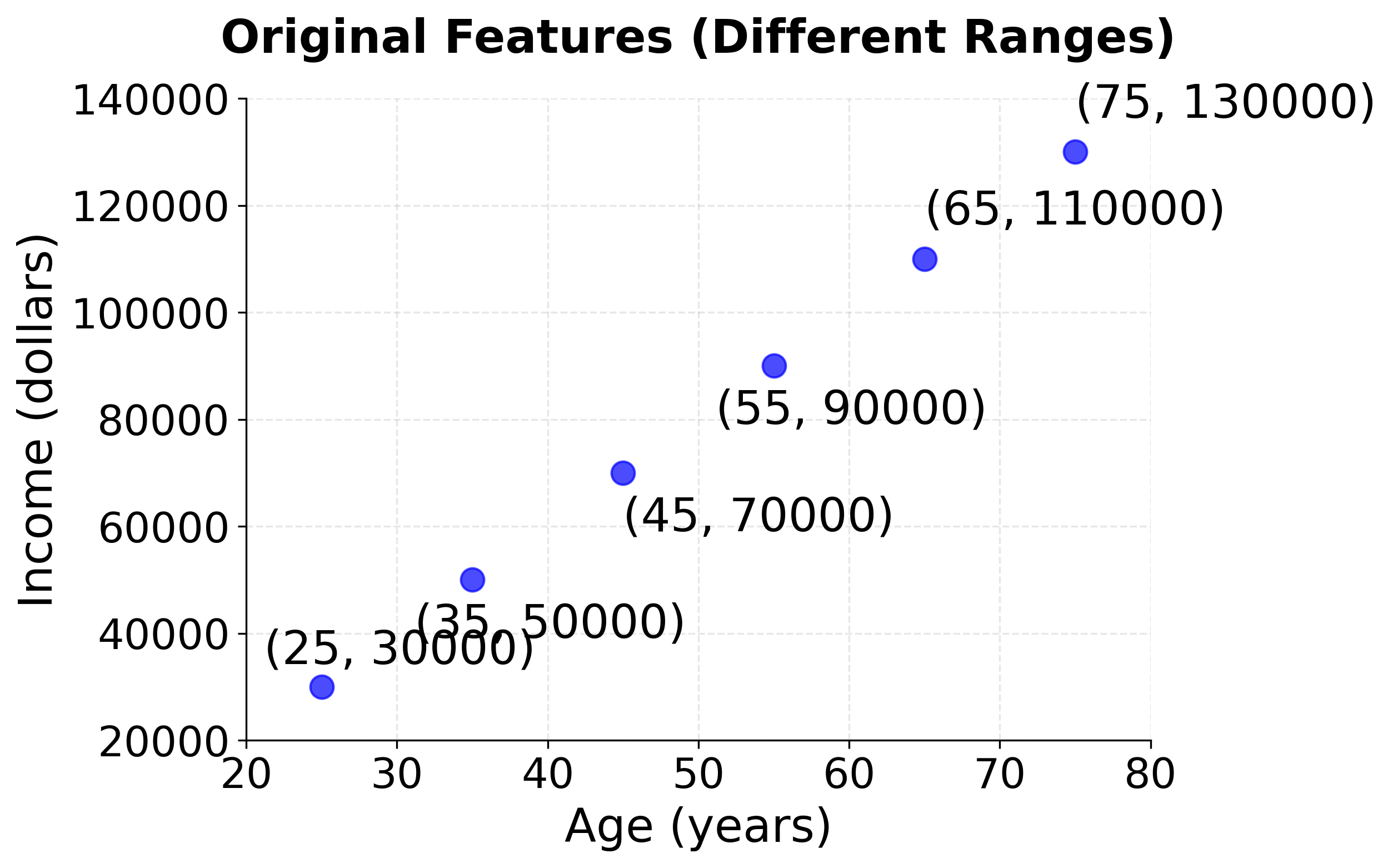
Example: Step-by-Step Calculation
Let's work through a detailed example with two features:
x1: age in years → [25, 35, 45, 55, 65, 75]x2: income in thousands → [30, 50, 70, 90, 110, 130]
Step 1: Calculate min and max values
- ,
- ,
Step 2: Apply normalization formula
For the first feature ():
For the second feature ():
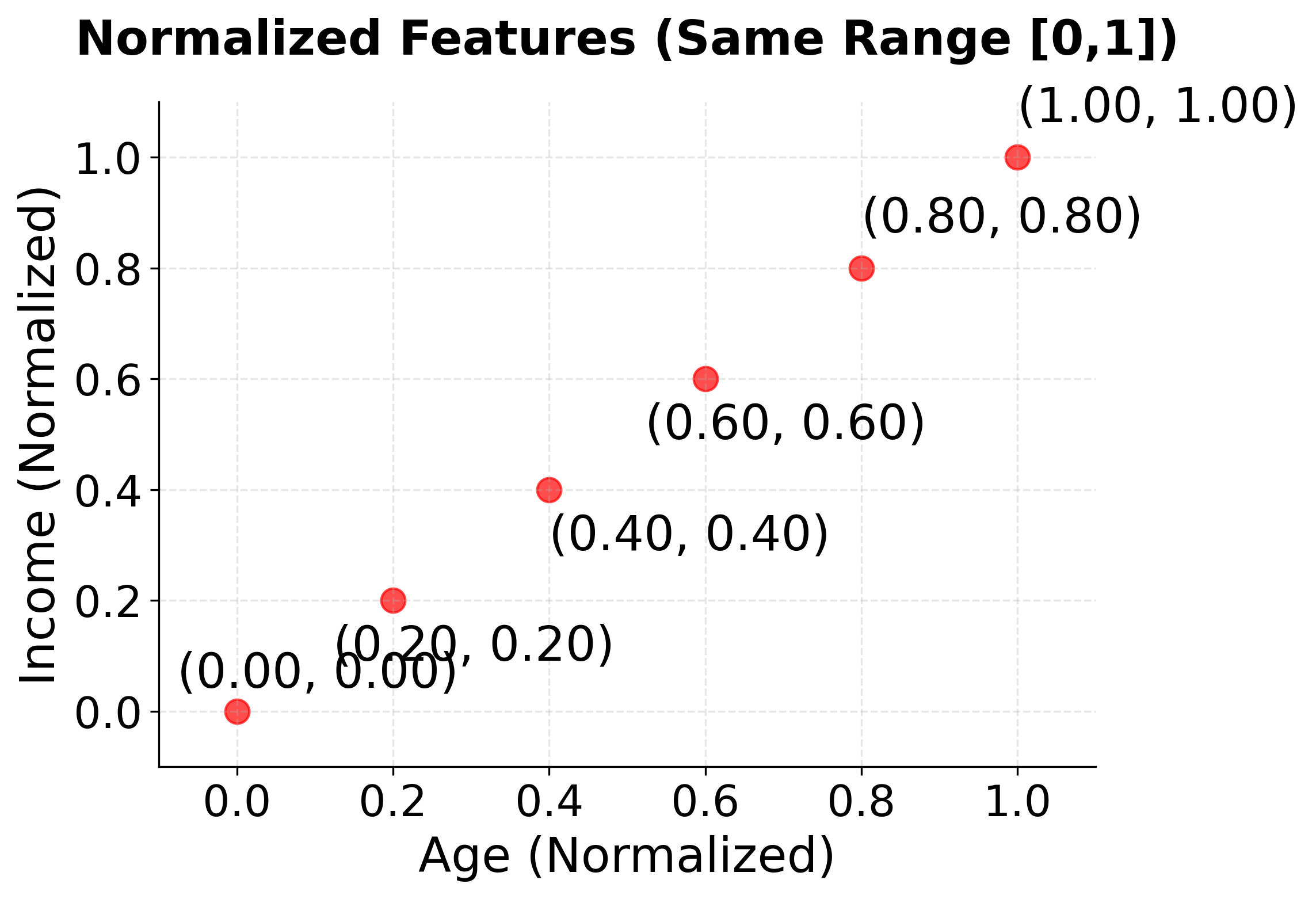
Result: Both features are now on the same [0, 1] scale:
x1: [25, 35, 45, 55, 65, 75] → [0.000, 0.200, 0.400, 0.600, 0.800, 1.000]x2: [30, 50, 70, 90, 110, 130] → [0.000, 0.200, 0.400, 0.600, 0.800, 1.000]
Practical Implementation
Proper Train-Test Split with Normalization
This example demonstrates the correct way to apply normalization in a machine learning pipeline:
Key Implementation Guidelines
Normalization is a simple but crucial step in the machine learning workflow. Here are the most important guidelines to follow:
-
Fit the scaler only on the training data.
This ensures that information from the test set does not leak into the model during training. Fitting on the entire dataset (including the test set) can lead to overly optimistic performance estimates and poor generalization. -
Transform both training and test data using the same scaler.
After fitting the scaler on the training data, use it to transform both the training and test sets. This guarantees that the scaling parameters (min and max values) are consistent and based solely on the training data. -
Never fit the scaler on the entire dataset before splitting.
Doing so introduces data leakage, as the test set statistics influence the scaling of the training data. -
Use pipelines to automate and safeguard the process.
Scikit-learn pipelines help ensure that normalization and modeling steps are applied correctly and in the right order, reducing the risk of data leakage and making your workflow more reproducible.
By following these guidelines, you ensure that your model evaluation is fair and that your results will generalize well to new, unseen data.
When to Use Normalization vs Standardization
Understanding when to use normalization versus standardization is crucial for optimal model performance:
Use Normalization (Min-Max Scaling) when:
- Neural Networks: Most neural network algorithms expect inputs in the range [0, 1] or [-1, 1]. Normalization ensures optimal activation function behavior.
- Image Processing: Pixel values are naturally bounded between 0 and 255, making normalization to [0, 1] intuitive.
- Distance-based algorithms: When you need to preserve the original distribution shape and want all features on the same bounded scale.
- Sparse data: When working with sparse matrices where standardization might create dense representations.
Use Standardization (Z-score scaling) when:
- Regularized regression: LASSO and Ridge regression assume features are on the same scale with mean 0.
- Principal Component Analysis: PCA is based on variance, so standardization ensures equal contribution from all features.
- Outlier presence: Standardization is more robust to outliers than normalization.
- Gaussian assumptions: When your algorithm assumes normally distributed features.
Key Differences: To clarify the differences between normalization and standardization, here’s a summary table and some explanatory notes:
| Aspect | Normalization | Standardization |
|---|---|---|
| Range | [0, 1] | Unbounded (can be any value, positive or negative) |
| Mean | Varies | 0 |
| Std Dev | Varies | 1 |
| Outlier Sensitivity | High | Lower (less sensitive) |
| Distribution Shape | Preserved | May change |
What does this mean in practice?
-
Normalization rescales your feature values so that everything fits between 0 and 1. Think of stretching or compressing the values to fit inside a box between 0 and 1, but the original shape and distribution of your data is preserved (unless you have extreme outliers, which can shrink everything else unnaturally). Use this when you want all features to be on the same scale, especially for neural nets or algorithms sensitive to value magnitudes.
-
Standardization transforms your data so that each feature has a mean of zero and a standard deviation of one. The values are spread out according to how they deviate from the average. This can make your data look more like a “bell curve” (Gaussian), but may actually change the distribution shape—especially for skewed data.
-
Outlier Sensitivity: Normalization is more affected by outliers because just one very large or very small value can set the min or max, squishing the rest of your data. Standardization handles outliers a bit better since it centers on the mean and spreads based on standard deviation.
When to use which?
- Use Normalization (Min-Max scaling) for image data, neural networks, or when features naturally fit in a bounded range.
- Use Standardization (Z-score scaling) for algorithms that assume data is centered (mean = 0), or when the data has outliers or Gaussian-like distributions.
If you’re unsure, try both and see which works better for your model!
Limitations and Considerations
When applying normalization, keep in mind several important limitations:
- Outlier sensitivity: Normalization is highly sensitive to outliers, as extreme values can compress the majority of data into a small range.
- Tip: Consider using robust scaling methods or removing outliers before normalization.
- Sparse data: For sparse matrices, normalization can convert the data into a dense format, which is inefficient and memory-intensive.
- Tip: Use
MinMaxScaler(feature_range=(0, 1))with sparse data carefully.
- Tip: Use
- Categorical variables: Do not normalize one-hot encoded or ordinal categorical variables, as this can destroy their intended meaning.
- Target variable: In most cases, avoid normalizing the target variable unless there is a specific reason to do so.
When applying normalization to your data, it's important to be aware of several common pitfalls that can affect the quality of your results and potentially introduce bias into your models. Understanding these issues in advance can help you avoid costly mistakes and ensure that your preprocessing pipeline is robust and reliable. Be aware of these common pitfalls:
- Data leakage: Fitting the scaler on the entire dataset (including the test set) introduces information from the test data into the training process, leading to overly optimistic performance estimates.
- Best practice: Always fit the scaler only on the training data, then use it to transform both the training and test sets.
- Inconsistent scaling: Using different scalers for training and test data can result in mismatched feature distributions.
- Over-normalization: Normalizing features that are already in the desired range can be unnecessary or even harmful.
- Categorical confusion: Normalizing categorical variables that should remain discrete can undermine their interpretability and utility.
For neural networks, you might want to use MinMaxScaler(feature_range=(-1, 1)) to center the data around zero, which can improve training stability for certain activation functions.
Practical Applications
Normalization plays a crucial role in a wide variety of real-world applications. For example, in computer vision tasks, it is common practice to rescale pixel values from their original range of [0, 255] down to [0, 1], which helps neural networks learn more effectively. Recommendation systems also benefit from normalization by bringing user ratings, item features, or interaction counts to a common scale, allowing algorithms to make fairer comparisons. In time series analysis, sensor readings that may be recorded in different units and scales are often normalized so that patterns can be more easily detected across multiple sensors. Natural language processing tasks involve working with features such as TF-IDF scores, document lengths, or word counts, all of which may be normalized to make the data more comparable across samples. Similarly, in financial modeling, normalization ensures that diverse features like stock prices, trading volumes, and economic indicators—all of which can have widely varying magnitudes—can be analyzed together on an equal footing.
Summary
Normalization is a fundamental preprocessing step that ensures features are treated fairly in machine learning algorithms. By transforming features to a common range, typically [0, 1], normalization:
- Enables fair comparison across variables with different ranges
- Improves the performance of neural networks and distance-based methods
- Prevents bias toward features with larger numeric ranges
- Stabilizes optimization by providing consistent input scales
The key to successful normalization is proper implementation: always fit the scaler on training data only, then transform both training and test sets using the fitted scaler. This prevents data leakage and ensures realistic model evaluation.
Choose normalization over standardization when working with neural networks, image data, or when you need to preserve the original distribution shape while ensuring all features contribute equally to the learning process.
Quiz
Ready to test your understanding of normalization? Take this quick quiz to reinforce what you've learned about min-max scaling.

Comments