InteractiveGauss-Markov Assumptions: Foundation of Linear Regression & OLS Estimation

Gauss-Markov Assumptions: The Foundation of Linear Regression

The Gauss-Markov assumptions are a set of conditions that, when satisfied, ensure that the ordinary least squares (OLS) estimator is the best linear unbiased estimator (BLUE). These assumptions form the theoretical foundation for linear regression and are crucial for understanding when OLS provides reliable results.

Introduction

Linear regression is one of the most fundamental tools in data science and statistics, but its validity depends on certain assumptions about the data and the underlying relationships. The Gauss-Markov assumptions, named after mathematicians Carl Friedrich Gauss and Andrey Markov, provide the conditions under which OLS estimation produces the most efficient and unbiased results. Understanding these assumptions is essential for proper model interpretation and for knowing when to apply alternative methods when assumptions are violated.

The Five Gauss-Markov Assumptions

The Gauss-Markov theorem states that under certain assumptions, the OLS estimator is the best linear unbiased estimator (BLUE). This means it has the smallest variance among all linear unbiased estimators. The five key assumptions are:

1. Linearity in Parameters

The first assumption stipulates that the model must be linear in its parameters, though not necessarily in the variables themselves. This means that each regression coefficient multiplies a variable, and the sum of these products (plus an intercept and the error term) forms the predicted value. The model must be written as:

$y_i = \beta_0 + \beta_1 x_{i1} + \beta_2 x_{i2} + \cdots + \beta_k x_{ik} + \varepsilon_i$

Here, $y_i$ is the dependent variable, $x_{ij}$ are independent variables, $\beta_j$ are coefficients to be estimated, and $\varepsilon_i$ is the error term. The model is allowed to include transformed variables (such as logarithms, polynomials, or interactions), as long as the equation remains linear in the β's. For example, $y = \beta_0 + \beta_1 x + \beta_2 x^2 + \varepsilon$ still satisfies this assumption. The implication is that OLS cannot, without modification, fit models where parameters appear in exponents, denominators, or other non-linear forms.

2. Random Sampling

This assumption requires that every observation in your sample is selected randomly and independently from the population of interest. In practical terms, this means each unit in the population has an equal probability of being included in the sample. Random sampling is crucial because it ensures that the sample represents the wider population and thus, that inferences drawn from the sample are valid. If random sampling is violated, estimates can be systematically biased, and standard errors may not accurately reflect sampling variability. Random sampling also implies independence: the value of one observation does not influence or provide information about another.

3. No Perfect Multicollinearity

This assumption requires that none of the independent variables is an exact linear function of any combination of the others. In other words, there must be no perfect or exact linear relationships among the explanatory variables. If perfect multicollinearity is present, it becomes mathematically impossible to estimate separate effects for the correlated variables using OLS, because the model cannot distinguish their individual influences. Even strong (but not perfect) correlations, known as high multicollinearity, can inflate the variances of the coefficient estimates, making statistical inference less reliable—coefficients can change erratically in response to small changes in the data. Ensuring that variables are linearly independent is essential for meaningful, stable regression results.

4. Zero Conditional Mean

This is one of the most critical assumptions for ensuring unbiasedness of the OLS estimates. It states that the error term has an expected value of zero given any values of the independent variables:

$E[\varepsilon_i | X] = 0$

In effect, this means there are no omitted variables, measurement errors, or functional misspecifications that systematically influence the error term. If this assumption is violated—if, for example, a relevant variable is left out and is correlated with the included regressors—then the OLS estimates will be biased and cannot be trusted for causal interpretation. Zero conditional mean also means that all the relevant information for predicting $y$ is contained in $X$; nothing is left in the error term that could be predicted by $X$.

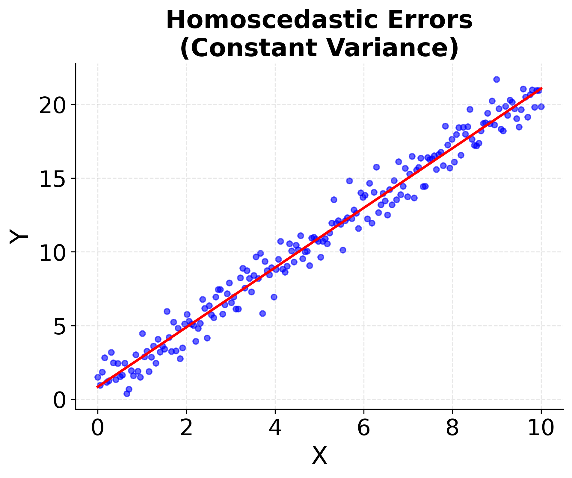
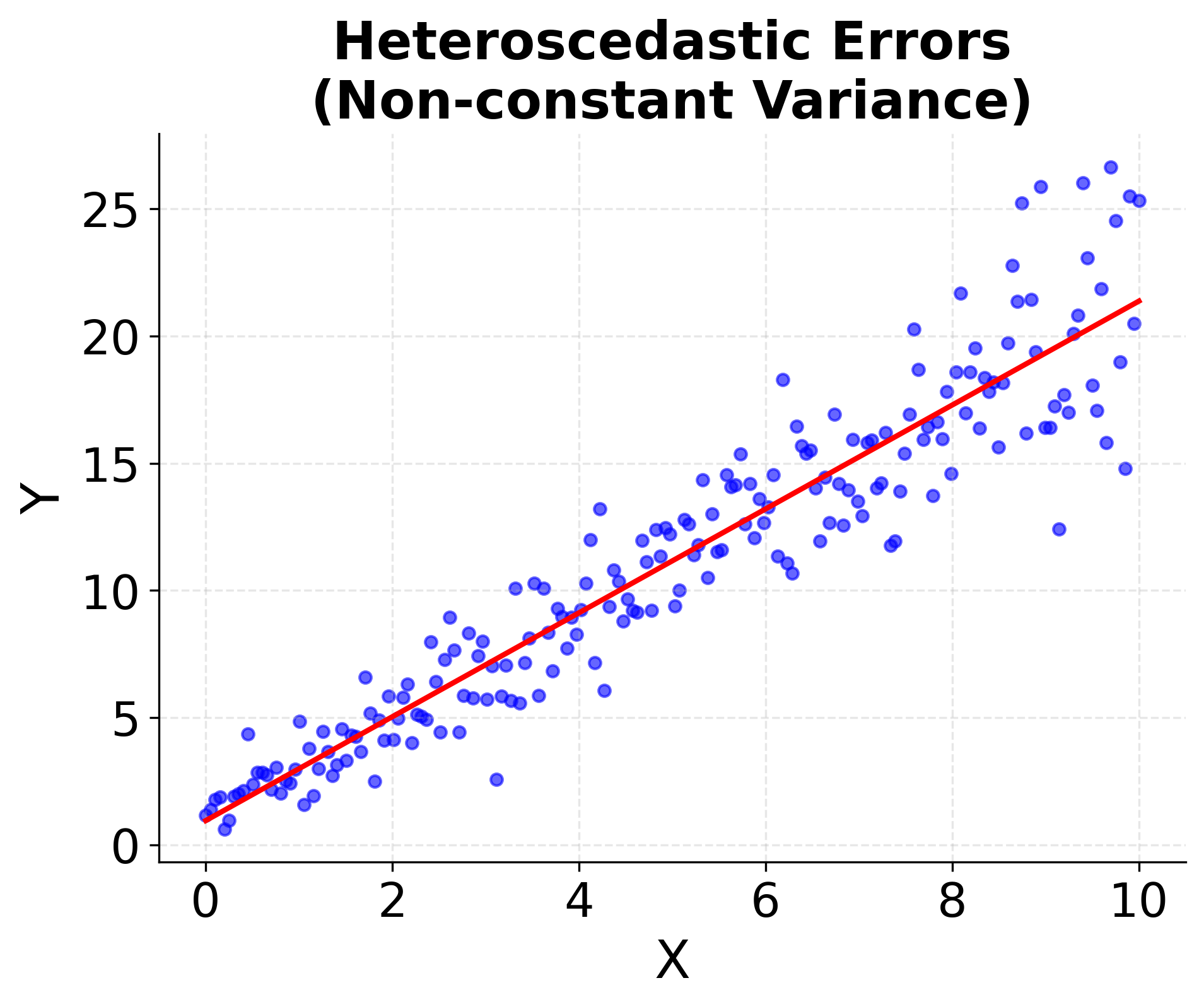
5. Homoscedasticity (Constant Variance)

This assumption posits that the variance of the error term is constant across all values of the independent variables:

$\text{Var}(\varepsilon_i | X) = \sigma^2$

This uniformity in error variance—called homoscedasticity—means that no matter what the values of $X$ are, the spread or "noise" around the regression line remains the same. When this assumption holds, the standard errors calculated for the coefficients are accurate and hypothesis tests (such as t-tests) can be trusted. When it is violated (a situation known as heteroscedasticity), the efficiency of the OLS estimator is compromised, and the standard errors can be biased, potentially leading to misleading statistical inferences. Detecting and correcting heteroscedasticity (for example, using robust standard errors or transforming variables) is an important part of regression diagnostics.

Mathematical Foundation

The Gauss-Markov theorem can be stated mathematically as follows:

Theorem: Under assumptions 1-5, the OLS estimator $\hat{\beta}$ is the best linear unbiased estimator (BLUE) of $\beta$.

This means:

• Unbiased: $E[\hat{\beta}] = \beta$
• Efficient: $\text{Var}(\hat{\beta})$ is the smallest among all linear unbiased estimators
• Consistent: As sample size increases, $\hat{\beta}$ converges to the true $\beta$

The OLS estimator is given by: $\hat{\beta} = (X'X)^{-1}X'y$

Where:

• $X$ is the matrix of independent variables
• $y$ is the vector of dependent variable
• $\hat{\beta}$ is the vector of estimated coefficients

Visualizing Assumption Violations

Understanding what happens when assumptions are violated is crucial for proper model diagnosis and selection of appropriate remedies.

Example: Homoscedasticity vs. Heteroscedasticity

This example demonstrates the difference between homoscedastic (constant variance) and heteroscedastic (non-constant variance) error terms:

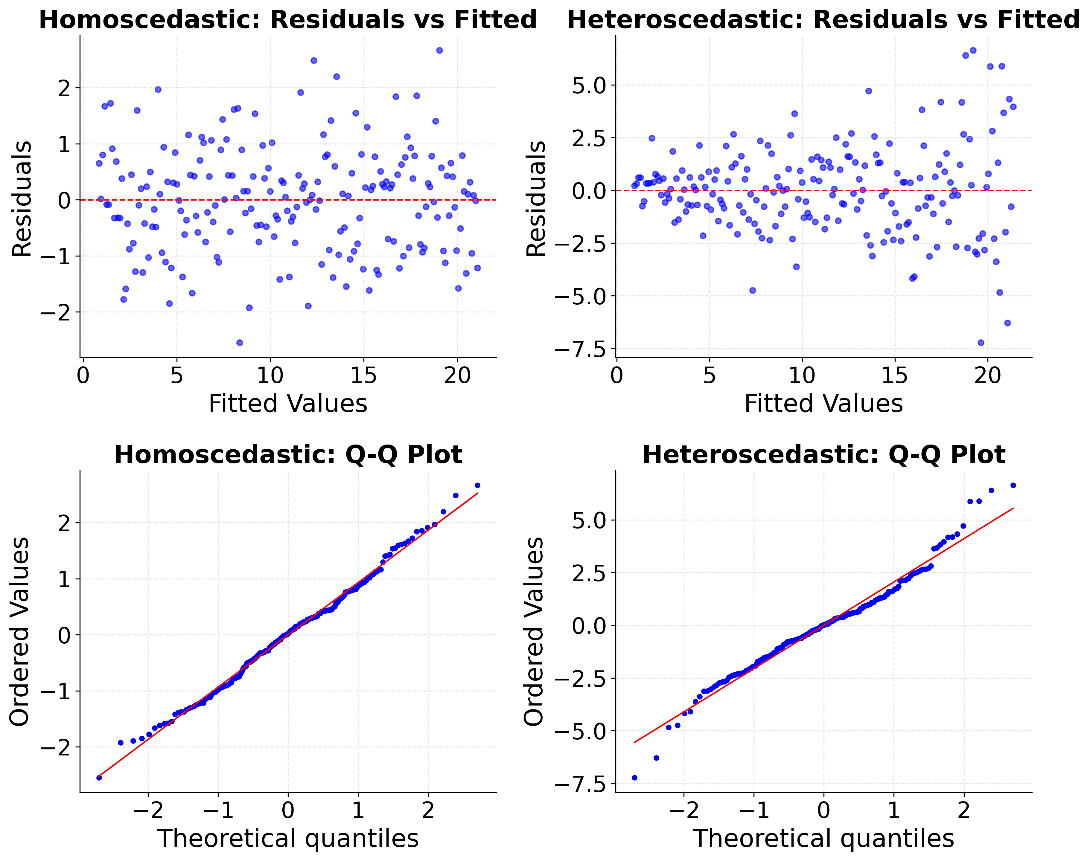
Example: Residual Plots for Assumption Testing

Residual plots are essential diagnostic tools for checking Gauss-Markov assumptions:

Key Components

The Gauss-Markov theorem underpins the theoretical foundation of Ordinary Least Squares (OLS) regression. It states that under five key assumptions—linearity in parameters, random sampling, no perfect multicollinearity, zero conditional mean, and homoscedasticity—the OLS estimator is the Best Linear Unbiased Estimator (BLUE) of the regression coefficients. This means that, among all estimators that are linear in the observed outcomes and unbiased, OLS yields the smallest possible variance.

Understanding and checking these assumptions is crucial because:

• If all assumptions are satisfied: OLS produces coefficient estimates with the lowest variance, and confidence intervals and p-values are reliable.
• If some assumptions are violated: OLS estimates may be biased, inefficient, or have standard errors that do not reflect true uncertainty, leading to invalid inference.

The practical approach involves:

• Diagnosing potential violations via plots and formal statistical tests,
• Understanding the consequences for estimation and inference,
• Applying remedies or alternative estimation techniques as needed (e.g., using robust standard errors, transforming variables, or specifying different models).

In applied regression analysis, routinely reviewing the Gauss-Markov assumptions and their diagnostics greatly increases the reliability and credibility of your statistical conclusions.

Assumption 1: Linearity in Parameters

• What it means: The relationship between variables can be expressed as a linear combination of parameters
• How to check: Plot residuals vs. fitted values; look for systematic patterns
• Violation consequences: Biased and inconsistent estimates
• Remedies: Transform variables, use polynomial terms, or switch to non-linear models

Assumption 2: Random Sampling

• What it means: Each observation is independently drawn from the population
• How to check: Examine data collection process, check for clustering or dependencies
• Violation consequences: Standard errors may be incorrect, affecting hypothesis tests
• Remedies: Use clustered standard errors, mixed-effects models, or account for sampling design

Assumption 3: No Perfect Multicollinearity

• What it means: Independent variables are not perfectly correlated
• How to check: Calculate correlation matrix, variance inflation factors (VIF)
• Violation consequences: OLS cannot be computed; high multicollinearity leads to unstable estimates
• Remedies: Remove redundant variables, use regularization (Ridge/Lasso), or collect more data

Assumption 4: Zero Conditional Mean

• What it means: Error term has zero expected value given the independent variables
• How to check: Test for omitted variable bias, use instrumental variables
• Violation consequences: Biased and inconsistent estimates
• Remedies: Include omitted variables, use instrumental variables, or switch to other estimation methods

Assumption 5: Homoscedasticity

• What it means: Error variance is constant across observations
• How to check: Plot residuals vs. fitted values, use Breusch-Pagan test
• Violation consequences: Inefficient estimates, incorrect standard errors
• Remedies: Use robust standard errors, weighted least squares, or transform variables

Interpretation Guidelines

When Assumptions Are Met

When the Gauss-Markov assumptions are fully satisfied, ordinary least squares (OLS) regression provides the best linear unbiased estimates of the coefficients. The resulting standard errors, confidence intervals, and hypothesis tests are all valid, supporting reliable inference. In this ideal scenario, model predictions are optimal and you can interpret OLS results with a high degree of confidence.

When Assumptions Are Violated

If one or more Gauss-Markov assumptions are violated, the properties of OLS estimation may be compromised. For example, when the relationship between variables is not linear in parameters, it may be necessary to transform variables or to use non-linear modeling approaches. Violations of random sampling often require analytic adjustments that explicitly account for dependencies or clustering present in the data. Multicollinearity, whether strong or perfect, can undermine the reliability of estimated coefficients; in such cases, regularization techniques or the removal of redundant variables may be warranted. If the zero conditional mean assumption does not hold—perhaps due to omitted variable bias—then including relevant omitted variables or switching to methods like instrumental variables can help address the issue. For problems of heteroscedasticity, where the error variance is not constant, robust standard errors or weighted least squares should be considered to obtain more reliable inference.

Diagnostic Tests

To effectively evaluate whether the assumptions hold, a range of diagnostic tools can be employed. Investigating linearity often starts with residual plots or statistical tests like the Ramsey RESET test. Checking for independence in errors can involve the Durbin-Watson or Breusch-Godfrey tests, which are especially relevant for time series or clustered data. Multicollinearity can be detected using the Variance Inflation Factor (VIF) or examining the correlation matrix among regressors. Assessing the zero conditional mean is less direct but can involve the Hausman test or procedures for detecting omitted variable bias. Finally, homoscedasticity can be evaluated by inspecting residual plots or conducting formal tests such as the Breusch-Pagan or White test.

Practical Applications

The Gauss-Markov assumptions not only provide theoretical assurance for OLS but also guide practical decision-making across fields.

In Data Science

A clear understanding of these assumptions aids critical choices throughout the data science workflow. When selecting models, knowledge of the assumptions helps you decide when linear regression is appropriate or when to turn to regularized or non-linear methods. If assumption violations are detected, this can prompt transformations or guide feature engineering. Diagnostic tests support model validation, ensuring reliability prior to real-world application or deployment.

In Business Analytics

In business contexts, adhering to Gauss-Markov assumptions helps guarantee the trustworthiness of predictive models used for forecasting and decision-making. These assumptions are also foundational when drawing causal inferences—knowing when regression supports causal claims is essential in strategic planning. For risk assessment and compliance, verifying model assumptions is often a regulatory requirement.

In Research

For scientific research, the assumptions guide experimental design to promote high-quality data collection that facilitates valid inference. Inference about hypotheses and the use of confidence intervals depend directly on the integrity of these assumptions. Moreover, rigorous statistical standards for publication often require transparency about how these foundational conditions are checked and addressed.

Limitations and Considerations

Common Violations

In practice, it is common to encounter situations where the Gauss-Markov assumptions are not entirely met. Many relationships in real-world data turn out to be non-linear, even when a linear approximation is convenient. Heteroscedasticity is frequent in economic or financial data, where variability may change with the level of explanatory variables. Time series and panel data regularly feature autocorrelation, breaking the independence assumption. Endogeneity, or correlation between variables and the error term, can also arise and threatens the validity of OLS estimates.

Robust Alternatives

When faced with assumption violations, alternative techniques are available. Heteroscedasticity can be handled with robust standard errors. For endogeneity, instrumental variable methods provide a solution. Autocorrelation may be addressed via generalized least squares. Non-linear relationships call for the adoption of non-linear models. When multicollinearity is present, methods such as Ridge or Lasso regression (regularization) can stabilize coefficient estimates.

Practical Considerations

It should be recognized that perfect adherence to every Gauss-Markov assumption is rare in real world analyses. Practitioners are encouraged to focus first on the most consequential violations affecting inference or prediction. Employing diagnostic tools facilitates the targeting of remedies to where they are most needed. Ultimately, decisions about how stringently to enforce each assumption should weigh the costs and benefits in context, balancing model complexity, interpretability, and credibility of results.

Summary

The Gauss-Markov assumptions provide the theoretical foundation for linear regression, ensuring that OLS produces the best linear unbiased estimates when conditions are met. Understanding these assumptions is crucial for:

• Proper Model Specification: Knowing when linear regression is appropriate
• Diagnostic Testing: Identifying assumption violations through residual analysis
• Remedy Selection: Choosing appropriate methods when assumptions are violated
• Result Interpretation: Understanding the reliability and limitations of estimates

While perfect adherence to all assumptions is rare in practice, awareness of these conditions enables data scientists to make informed decisions about model selection, diagnostic testing, and result interpretation. The key is to identify the most critical violations and apply appropriate remedies to ensure reliable and valid statistical inference.

Quiz

Ready to test your understanding of the Gauss-Markov assumptions? Challenge yourself with this quiz to see how well you've grasped these fundamental concepts of linear regression. Good luck!