InteractiveStatistical Inference: Drawing Conclusions from Data - Complete Guide with Estimation & Hypothesis Testing

Statistical Inference: Drawing Conclusions from Data

Statistical inference is the process of using sample data to draw conclusions about populations, enabling data scientists to make decisions under uncertainty. Through estimation and hypothesis testing, inference provides the rigorous mathematical foundation for turning observations into actionable insights about the world.

Introduction

Every data science project begins with a fundamental challenge: we have access only to a sample of data, yet we need to make claims about entire populations or underlying processes. Statistical inference bridges this gap by providing principled methods for quantifying uncertainty and drawing valid conclusions despite incomplete information. Whether estimating average customer lifetime value from a survey, testing whether a new feature improves user engagement, or determining which factors truly influence outcomes, inference techniques transform raw data into reliable knowledge.

The field of statistical inference rests on probability theory and sampling distributions, which formalize how sample statistics behave when drawn from populations. When we collect a random sample and calculate its mean, that sample mean is itself a random variable with its own distribution. Understanding these sampling distributions allows us to construct confidence intervals that capture population parameters with known probability, and to perform hypothesis tests that control error rates in a principled manner.

This chapter explores the core concepts of statistical inference, beginning with estimation approaches for quantifying population parameters, then moving to hypothesis testing frameworks for evaluating claims. We'll examine how to interpret p-values correctly, understand different types of errors that can occur in hypothesis testing, and apply common statistical tests appropriate for various data scenarios. Throughout, we'll emphasize not just mechanical procedures but the reasoning and interpretation that make inference a powerful tool for data-driven decision making.

Estimation: Quantifying Population Parameters

Estimation involves using sample data to approximate unknown population parameters. When we cannot measure an entire population (whether due to cost, time constraints, or physical impossibility), we rely on samples to provide our best guesses about population characteristics like means, proportions, or variances.

Point Estimation

Point estimation produces a single value as the estimate of a population parameter. The sample mean serves as a point estimate of the population mean, just as the sample proportion estimates the population proportion. For instance, if we survey 500 customers and find an average satisfaction score of 7.8 out of 10, that 7.8 represents our point estimate of the true average satisfaction across all customers.

Point estimators have desirable statistical properties when chosen carefully. An unbiased estimator produces estimates that equal the true parameter value on average across repeated sampling. The sample mean is unbiased for the population mean: if we drew many samples and calculated their means, those sample means would center around the true population mean. Consistency ensures that estimates converge to the true value as sample size increases, while efficiency means the estimator has minimal variance among all unbiased options.

Despite their simplicity and ease of communication, point estimates carry a significant limitation: they provide no information about uncertainty. Reporting that average customer satisfaction is 7.8 leaves critical questions unanswered. How confident can we be in this number? Might the true average be 7.5 or 8.1? This motivates the need for interval estimation.

Interval Estimation: Confidence Intervals

Confidence intervals provide a range of plausible values for a population parameter, quantifying the uncertainty inherent in estimation. A 95% confidence interval for the population mean might be [7.5, 8.1], indicating that based on our sample data and the inferential procedure used, we can be 95% confident that the true population mean falls within this range.

The interpretation of confidence levels requires care. A 95% confidence level means that if we repeated the sampling process many times and constructed a confidence interval from each sample using the same procedure, approximately 95% of those intervals would contain the true population parameter. It does not mean there is a 95% probability that the true parameter lies in our specific observed interval: the parameter is fixed, and either our interval captures it or it doesn't. The probability statement refers to the long-run behavior of the interval construction procedure.

Confidence intervals are constructed using the sampling distribution of the estimator. For a population mean with known variance, the confidence interval takes the form:

Where:

• $\bar{x}$: Sample mean
• $z_{\alpha/2}$: Critical value from the standard normal distribution (e.g., 1.96 for 95% confidence)
• $\sigma$: Population standard deviation
• $n$: Sample size

When the population variance is unknown, as is typical in practice, we replace $\sigma$ with the sample standard deviation $s$ and use the t-distribution instead of the normal distribution:

The t-distribution accounts for the additional uncertainty from estimating the variance, with heavier tails than the normal distribution that provide wider intervals for small samples.

Several factors influence confidence interval width. Larger sample sizes reduce the standard error term $s/\sqrt{n}$, yielding narrower intervals that reflect increased precision. Higher confidence levels require larger critical values, widening intervals to maintain the desired coverage probability. Greater variability in the population (larger $s$) produces wider intervals because the data provide less precise information about the center.

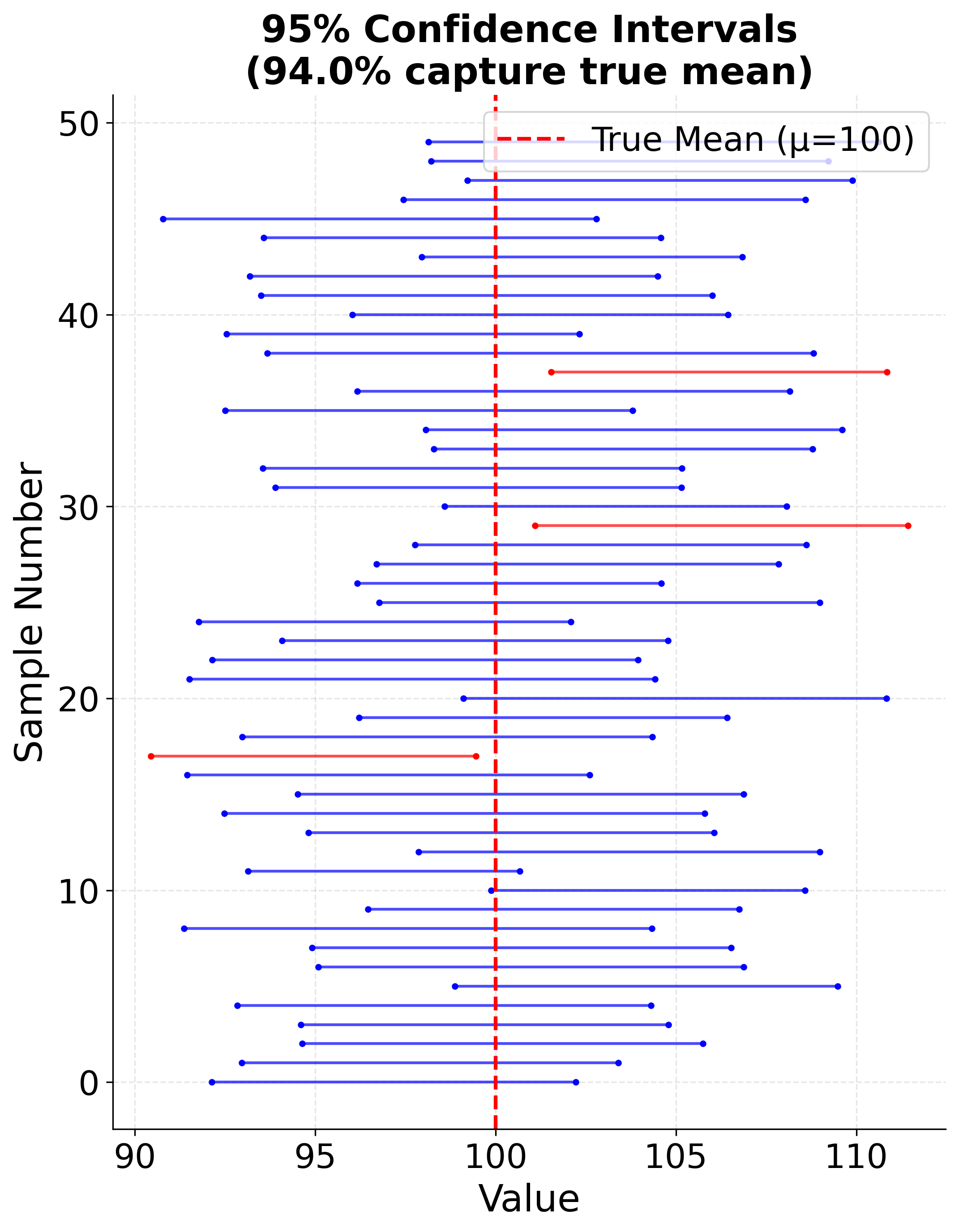
Example: Confidence Intervals Across Multiple Samples

This visualization demonstrates the interpretation of confidence intervals by showing multiple 95% confidence intervals constructed from different samples of the same population. Approximately 95% of the intervals contain the true population mean.

Hypothesis Testing: Evaluating Claims

While estimation focuses on approximating parameter values, hypothesis testing evaluates specific claims or hypotheses about populations. This framework allows researchers to determine whether observed data provide sufficient evidence to reject a stated hypothesis, controlling error rates in a rigorous manner.

The Hypothesis Testing Framework

Hypothesis testing begins by formulating two competing hypotheses. The null hypothesis ($H_0$) represents a default position, skeptical claim, or status quo that we seek evidence against. The alternative hypothesis ($H_1$ or $H_a$) represents the research hypothesis or claim we wish to establish. For example, when testing whether a new teaching method improves test scores compared to the standard approach, the null hypothesis might state that the methods produce equal average scores, while the alternative claims the new method yields higher scores.

The logic of hypothesis testing follows a proof-by-contradiction structure. We assume the null hypothesis is true, then calculate how likely the observed data (or more extreme data) would be under this assumption. If the data would be highly unlikely under the null hypothesis, we have evidence to reject it in favor of the alternative. If the data are reasonably consistent with the null hypothesis, we fail to reject it, though importantly, this does not prove the null hypothesis true.

Test Statistics and P-values

A test statistic summarizes how far the sample data deviate from what the null hypothesis predicts, measured in standard error units. For testing a population mean, the t-statistic is commonly used:

Where:

• $\bar{x}$: Sample mean
• $\mu_0$: Hypothesized population mean under $H_0$
• $s$: Sample standard deviation
• $n$: Sample size

This statistic measures how many standard errors the sample mean lies from the hypothesized value. Large absolute values of the test statistic indicate data that would be unusual if the null hypothesis were true.

The p-value quantifies the strength of evidence against the null hypothesis. Formally, the p-value is the probability of observing a test statistic at least as extreme as the one calculated from the sample data, assuming the null hypothesis is true. A small p-value indicates that the observed data would be quite unlikely under the null hypothesis, providing evidence against it.

Common misinterpretations of p-values plague statistical practice. The p-value is not the probability that the null hypothesis is true (that probability is either 0 or 1, though unknown to us). Nor is one minus the p-value the probability that the alternative hypothesis is true. The p-value also does not measure the size or importance of an effect; even trivial differences can yield tiny p-values with sufficiently large samples. Rather, the p-value simply measures how compatible the data are with the null hypothesis.

Significance Levels and Decision Rules

The significance level $\alpha$ (alpha) sets a threshold for decision making. Common choices include $\alpha = 0.05$ or $\alpha = 0.01$. If the p-value falls below $\alpha$, we reject the null hypothesis and declare the result "statistically significant." If the p-value exceeds $\alpha$, we fail to reject the null hypothesis.

The significance level represents the maximum Type I error rate we are willing to tolerate. It should be chosen before conducting the test based on the consequences of different types of errors in the specific context, not after seeing the data. Conventions like $\alpha = 0.05$ are merely defaults; situations with severe consequences for false positives might warrant more stringent levels like $\alpha = 0.01$, while exploratory analyses might use $\alpha = 0.10$.

Type I and Type II Errors

Hypothesis testing involves making decisions under uncertainty, which inevitably leads to the possibility of errors. A Type I error occurs when we reject a true null hypothesis, a "false positive" that claims an effect exists when it does not. The probability of a Type I error equals the significance level $\alpha$, which we control directly by our choice of threshold.

A Type II error occurs when we fail to reject a false null hypothesis, a "false negative" that misses a real effect. The probability of a Type II error is denoted $\beta$ (beta) and depends on the true parameter value, sample size, and significance level. The power of a test, defined as $1 - \beta$, represents the probability of correctly rejecting a false null hypothesis. Higher power means the test is more likely to detect true effects when they exist.

These error types reflect a fundamental tradeoff. Making it harder to commit Type I errors (lowering $\alpha$) simultaneously makes Type II errors more likely unless we increase sample size. The appropriate balance depends on the relative costs of each error type in context. Medical screening tests for serious diseases might prioritize avoiding Type II errors (missing true cases) even at the cost of more Type I errors (false alarms), while legal systems traditionally emphasize minimizing Type I errors (false convictions) accepting higher Type II error rates (wrongful acquittals).

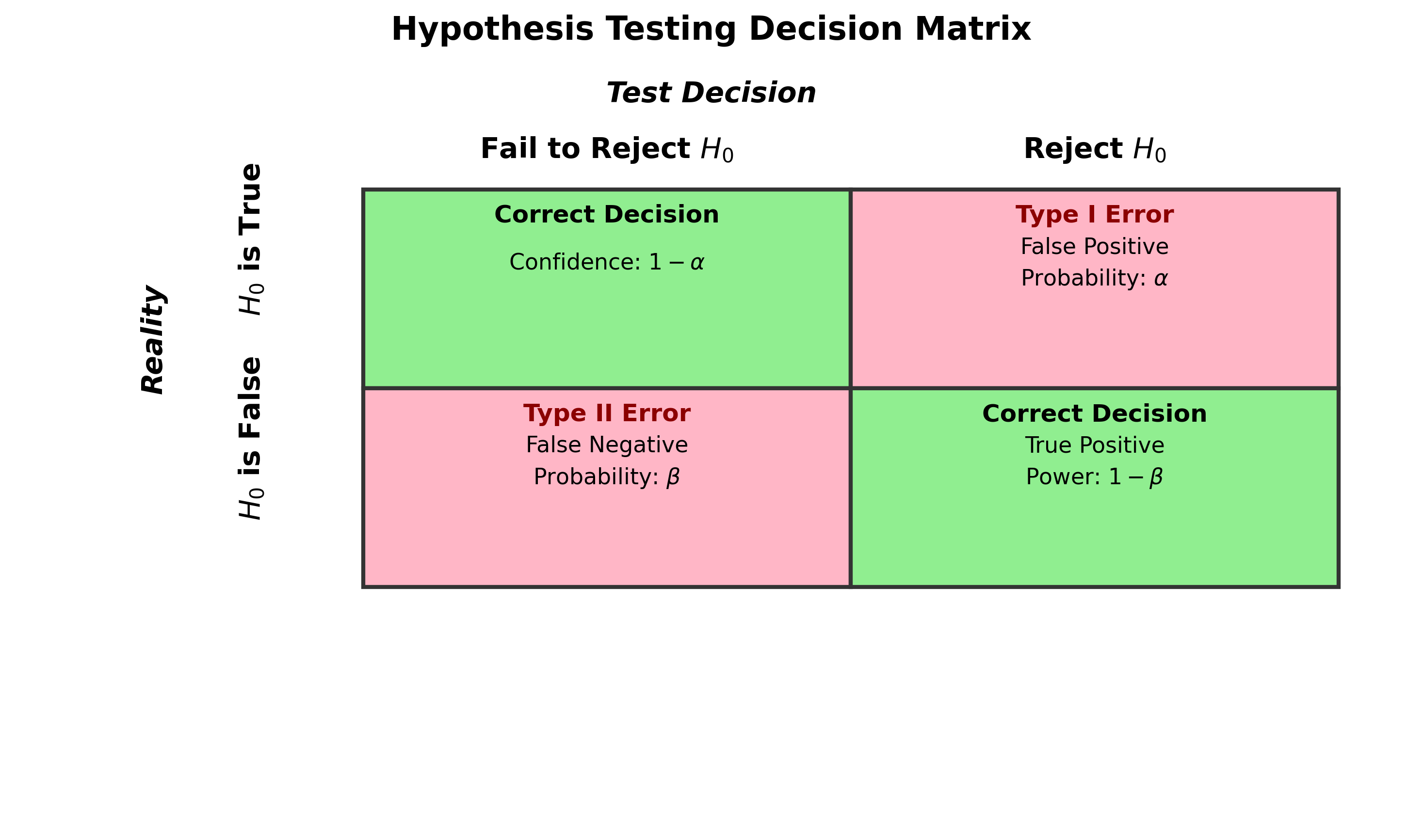
Example: Decision Matrix for Hypothesis Testing

The following matrix shows the four possible outcomes in hypothesis testing, illustrating how Type I and Type II errors relate to the true state of the world and our test decision.

Example: Visualizing Hypothesis Testing Concepts

The following visualizations demonstrate the relationship between sampling distributions under the null and alternative hypotheses, showing how significance levels, test statistics, and power relate to each other.

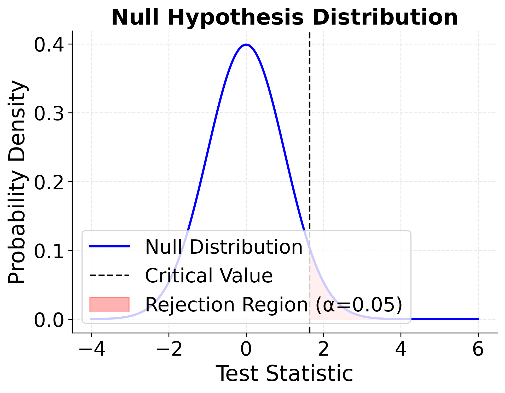
The first plot shows the sampling distribution assuming the null hypothesis is true. When we conduct a hypothesis test, we calculate a test statistic from our sample data and compare it to the critical value (the vertical dashed line). If our test statistic falls in the rejection region (shaded in red), we reject the null hypothesis. The size of this rejection region corresponds to our chosen significance level α, which represents the probability of Type I error—rejecting the null hypothesis when it is actually true.

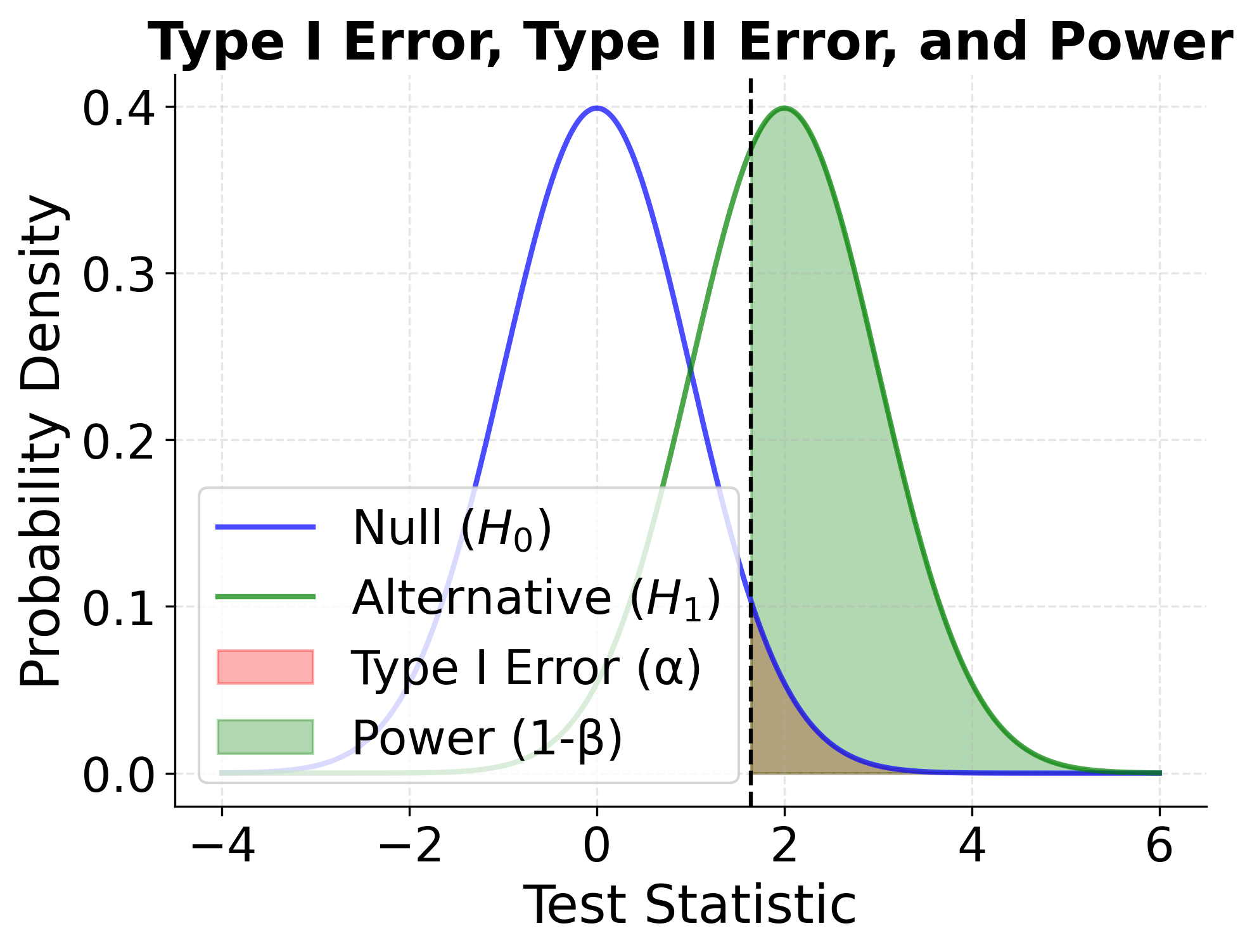
The second plot is more complex but crucial for understanding hypothesis testing. It shows two overlapping probability distributions representing two different states of reality:

• Blue curve (Null hypothesis $H_0$): This represents the distribution of test statistics we would observe if the null hypothesis were actually true (no effect exists).
• Green curve (Alternative hypothesis $H_1$): This represents the distribution of test statistics we would observe if the alternative hypothesis were true (an effect does exist).

The vertical dashed line represents our decision boundary—the critical value. Everything to the right of this line is the rejection region where we decide to reject $H_0$.

Understanding the shaded regions:

• Red shaded area (under blue curve, right of critical value): This is Type I error probability (α = 0.05). It shows how often we would incorrectly reject the null hypothesis when it is actually true. This area represents false positives.
• Green shaded area (under green curve, right of critical value): This is statistical power (1 - β). It shows how often we would correctly reject the null hypothesis when the alternative is true. This represents true positives—successfully detecting a real effect.
• Unshaded portion of green curve (left of critical value): This is Type II error probability (β). It shows how often we would fail to reject the null hypothesis when the alternative is actually true. This represents false negatives—missing a real effect.

The key insight is the tradeoff: if we move the critical value to the left (making it easier to reject $H_0$), we increase power but also increase Type I error. If we move it to the right (making it harder to reject $H_0$), we decrease Type I error but also decrease power (increase Type II error). The only way to improve both simultaneously is to increase the sample size, which makes both distributions narrower and more separated.

Common Statistical Tests

Statistical inference provides a rich toolkit of tests designed for different data types and research questions. Selecting the appropriate test requires understanding the data structure, distributional assumptions, and hypotheses being evaluated.

T-Tests: Comparing Means

T-tests evaluate hypotheses about population means and come in several variants. The one-sample t-test determines whether a population mean differs from a hypothesized value, such as testing whether average customer spending differs from $50. The independent samples t-test compares means between two separate groups, like comparing average test scores between students taught with different methods. The paired samples t-test analyzes differences within matched pairs, such as before-and-after measurements on the same individuals.

T-tests assume that data are approximately normally distributed, though they are fairly robust to moderate departures from normality, especially with larger sample sizes (typically n > 30). For severely non-normal data or small samples, nonparametric alternatives like the Wilcoxon tests may be more appropriate. T-tests also assume equal variances between groups for the independent samples variant, though Welch's t-test provides a modification that relaxes this assumption.

Chi-Square Tests: Analyzing Categorical Data

Chi-square tests evaluate relationships and distributions in categorical data. The chi-square goodness-of-fit test determines whether observed frequencies of categories match expected frequencies under some hypothesis. For example, we might test whether the distribution of customer age groups in our sample matches the known distribution in the general population.

The chi-square test of independence evaluates whether two categorical variables are independent or associated. When analyzing a contingency table of social media platform usage by age group, this test would determine whether platform preference depends on age or whether the variables are independent. The test compares observed cell frequencies to frequencies expected under independence, with large discrepancies providing evidence of association.

Chi-square tests require adequate sample sizes for valid inference. A common rule of thumb suggests expected frequencies should exceed 5 in each cell, though this guideline can be relaxed for larger tables. When expected frequencies are too small, exact tests like Fisher's exact test provide alternatives.

ANOVA: Comparing Multiple Groups

Analysis of variance (ANOVA) extends t-tests to compare means across three or more groups simultaneously. Rather than conducting multiple pairwise t-tests, which inflates Type I error rates, ANOVA tests the overall null hypothesis that all group means are equal against the alternative that at least one differs.

ANOVA partitions total variance into components: variance between groups (reflecting true differences in group means plus random error) and variance within groups (reflecting only random error). The F-statistic compares these variance components, with large values indicating that between-group variance exceeds what random chance alone would produce, suggesting real differences in population means.

When ANOVA rejects the null hypothesis, it indicates that not all means are equal but doesn't identify which specific groups differ. Post-hoc tests like Tukey's HSD provide pairwise comparisons while controlling family-wise error rates. ANOVA assumes normally distributed data within groups, equal variances across groups (homoscedasticity), and independent observations. Violations may require transformations or alternative approaches like Kruskal-Wallis tests.

Correlation Tests: Measuring Relationships

Correlation tests evaluate the strength and significance of relationships between continuous variables. Pearson correlation measures linear associations, producing correlation coefficients (r) ranging from -1 (perfect negative correlation) through 0 (no linear relationship) to +1 (perfect positive correlation). Hypothesis tests determine whether observed correlations differ significantly from zero, indicating genuine population-level associations rather than random sample fluctuations.

Pearson correlation assumes bivariate normality and is sensitive to outliers. Spearman's rank correlation provides a nonparametric alternative that evaluates monotonic relationships using ranks rather than raw values, making it robust to outliers and appropriate for ordinal data. Both measures capture association strength, not causation: significant correlations may reflect confounding variables or reverse causality rather than direct causal effects.

Practical Considerations in Statistical Inference

Applying statistical inference effectively requires attention to several practical considerations beyond mechanical test execution. Sample size planning through power analysis helps ensure studies can detect effects of meaningful magnitude with acceptable probability. Researchers should determine required sample sizes before data collection based on expected effect sizes, desired power (typically 0.80), and chosen significance levels.

The distinction between statistical significance and practical significance deserves emphasis. With sufficiently large samples, even trivial effects yield tiny p-values and "significant" results. Conversely, important effects may fail to reach significance in underpowered studies. Effect sizes and confidence intervals provide crucial context about the magnitude and precision of estimates beyond binary significant/not-significant classifications.

Multiple testing issues arise when conducting many tests simultaneously, as performing 20 independent tests at α = 0.05 yields an expected one false positive even when all null hypotheses are true. Bonferroni corrections and false discovery rate procedures control family-wise or expected error rates across multiple comparisons. Exploratory analyses generating hypotheses should be distinguished from confirmatory analyses testing pre-specified hypotheses, with appropriate adjustment for multiplicity in the latter.

Summary

Statistical inference provides the foundational framework for making rigorous conclusions about populations based on sample data. Through estimation, we quantify population parameters and the uncertainty surrounding them, using point estimates for precision and confidence intervals to capture ranges of plausible values. Hypothesis testing complements estimation by evaluating specific claims, allowing us to determine whether data provide sufficient evidence against null hypotheses while controlling error rates.

The mechanics of inference rest on understanding sampling distributions, which describe how statistics vary across repeated samples. This probabilistic foundation enables proper interpretation of confidence levels and p-values, though both are frequently misunderstood. Confidence levels describe long-run coverage rates of interval procedures, while p-values measure data compatibility with null hypotheses rather than hypothesis probabilities.

Selecting appropriate inferential methods requires matching tests to research questions and data characteristics. T-tests compare means, chi-square tests analyze categorical associations, ANOVA handles multiple group comparisons, and correlation tests measure relationships. Each carries assumptions about data distributions and structure that must be verified for valid inference. Beyond mechanical application, effective inference demands careful interpretation that distinguishes statistical significance from practical importance, accounts for multiple testing, and recognizes the limits of what statistical tests can and cannot demonstrate. These principles transform inference from rote calculation into a powerful reasoning tool that enables data-driven discovery while maintaining appropriate epistemic humility about conclusions drawn from uncertain data.

Quiz

Ready to test your understanding of statistical inference? Challenge yourself with the following quiz covering estimation, confidence intervals, hypothesis testing, and common statistical tests. Good luck!