Central Limit Theorem: Foundation of Statistical Inference & Sampling Distributions

The Central Limit Theorem (CLT) is one of the most fundamental results in probability theory and statistics. It states that the distribution of sample means approximates a normal distribution as the sample size becomes larger, regardless of the population's original distribution. This remarkable property underpins much of statistical inference and hypothesis testing.

In simpler terms, imagine you're measuring the heights of people in a city. If you take small groups of people and calculate the average height of each group, something magical happens: even if the individual heights aren't perfectly bell-shaped, the averages of those groups will form a nice, symmetric bell curve. The more people you include in each group, the more perfect that bell curve becomes. This is why working with averages is so powerful: they're predictable and well-behaved, even when the underlying data is messy or skewed.

The Central Limit Theorem bridges the gap between theoretical probability and practical data analysis. When we collect samples from a population and calculate their means, the CLT shows that even if the original population has a skewed, uniform, or any other non-normal distribution, the distribution of those sample means will tend toward a normal distribution as we increase the sample size.

This convergence to normality has important implications for data science and statistics. It explains why the normal distribution appears so frequently in nature and in data analysis, and it justifies the use of normal-based inferential methods even when working with populations that are not normally distributed. The theorem provides the theoretical foundation for confidence intervals, hypothesis tests, and many machine learning algorithms that assume normally distributed errors or parameters.

Understanding the Central Limit Theorem enables you to make probabilistic statements about sample statistics, quantify uncertainty in estimates, and apply powerful parametric methods to a wide variety of real-world problems. This chapter explores the mathematical statement of the theorem, demonstrates its behavior through visual examples, and discusses its practical applications and limitations.

The Central Limit Theorem can be stated formally as follows. Let $X_1, X_2, \ldots, X_n$ be a sequence of independent and identically distributed (i.i.d.) random variables with mean $\mu$ and finite variance $\sigma^2$. Define the sample mean as:

Then, as the sample size $n$ approaches infinity, the standardized sample mean converges in distribution to a standard normal distribution:

This can be equivalently stated as:

Where:

• $\bar{X}_n$: Sample mean of $n$ observations
• $\mu$: Population mean (expected value of $X_i$)
• $\sigma^2$: Population variance
• $\sigma / \sqrt{n}$: Standard error of the mean
• $N(0, 1)$: Standard normal distribution
• $\xrightarrow{d}$: Converges in distribution

The key insight here is that the standard error of the mean decreases at a rate proportional to $1/\sqrt{n}$. This means that as we collect more data, our estimate of the population mean becomes more precise, and the distribution of sample means becomes increasingly concentrated around the true population mean.

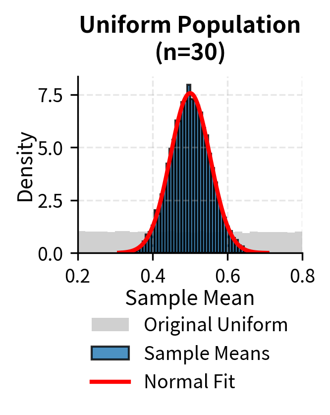
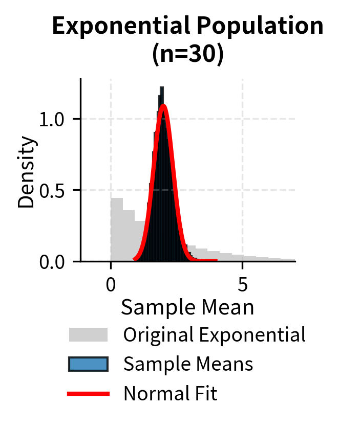
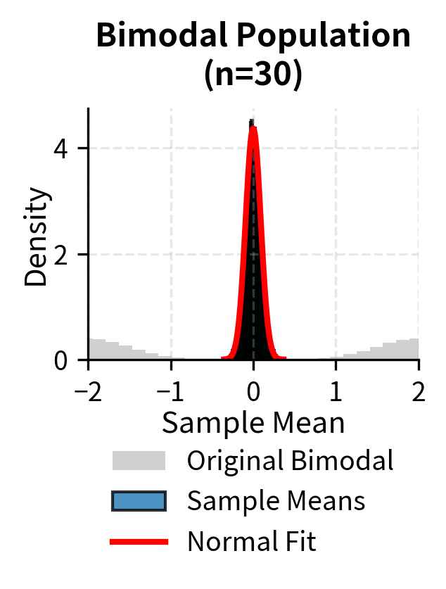
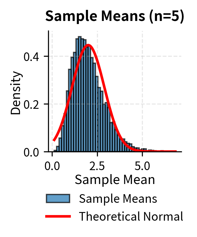
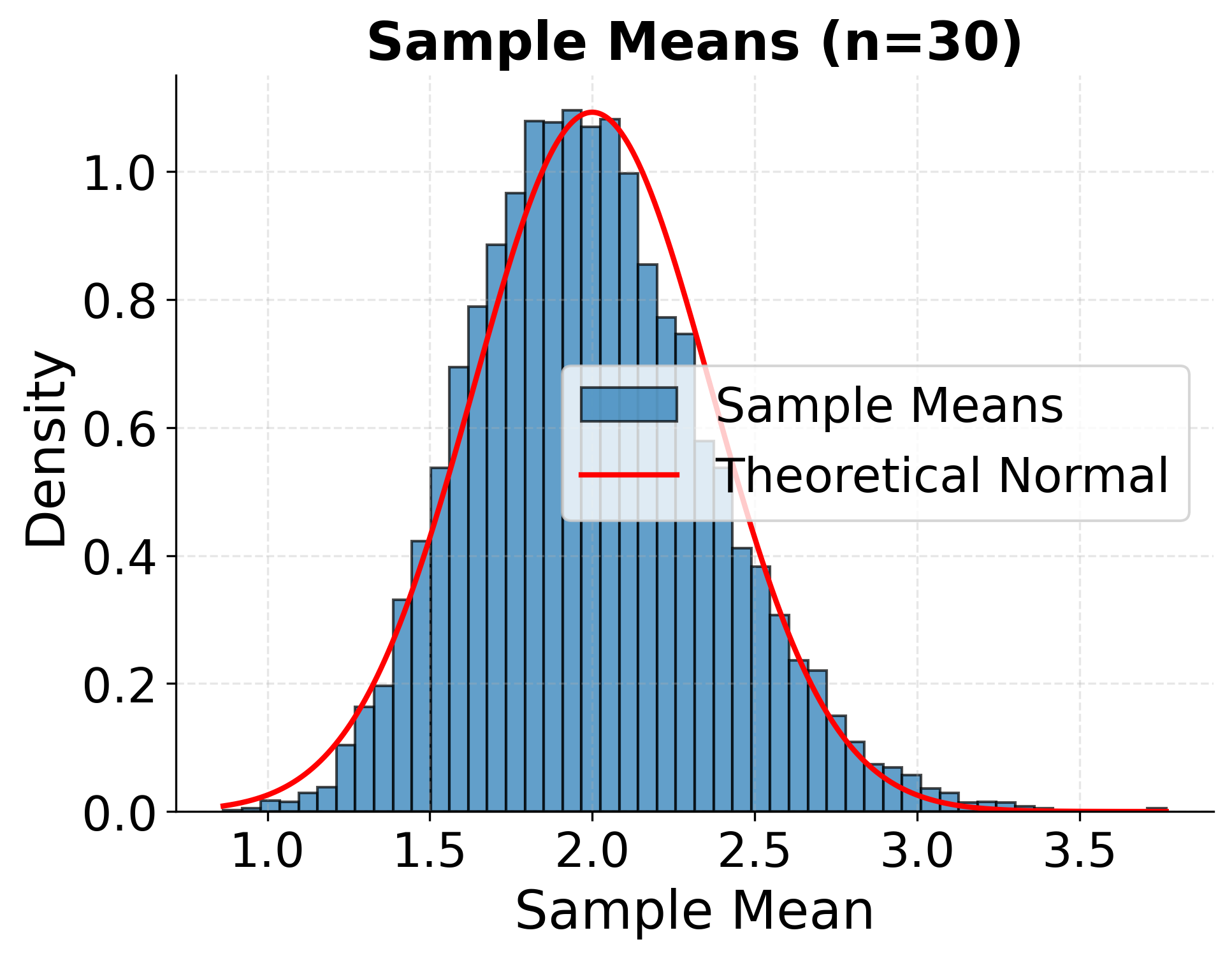
To illustrate that the Central Limit Theorem applies regardless of the original population distribution, the following examples show convergence to normality for uniform, exponential, and bimodal populations:

A critical component of the Central Limit Theorem is the standard error of the mean, which quantifies the variability of sample means around the population mean. The standard error is defined as:

This formula reveals an important relationship between sample size and precision. Doubling the sample size does not double the precision; rather, it improves precision by a factor of $\sqrt{2} \approx 1.41$. To cut the standard error in half and achieve twice the precision, we need to quadruple the sample size. This square-root relationship has practical implications for study design and resource allocation in research projects.

In practice, the population standard deviation $\sigma$ is typically unknown and must be estimated from the sample using the sample standard deviation $s$. When we substitute $s$ for $\sigma$, we obtain the estimated standard error:

The use of the estimated standard error leads to the Student's t-distribution rather than the normal distribution for small samples, but as sample size increases, the t-distribution converges to the normal distribution, consistent with the Central Limit Theorem.

A common practical question is: how large must the sample size be for the Central Limit Theorem to apply? The answer depends on the shape of the original population distribution. For populations that are already approximately normal, even small sample sizes like $n = 5$ or $n = 10$ can produce sample means that are approximately normally distributed. For symmetric but non-normal distributions, moderate sample sizes around $n = 30$ are typically sufficient.

However, when the population distribution is highly skewed or has heavy tails, larger sample sizes may be required before the sample means converge to normality. In cases of extreme skewness, sample sizes of $n = 100$ or more might be necessary. The conventional rule of thumb that $n \geq 30$ is sufficient for the CLT to apply should be viewed as a guideline rather than a hard requirement, and you should consider the shape of your data when determining appropriate sample sizes.

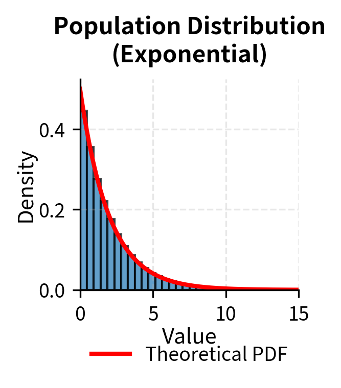
The following example demonstrates how the distribution of sample means becomes increasingly normal as sample size increases, starting from a highly skewed exponential distribution:

The Central Limit Theorem provides the mathematical foundation for nearly all of classical statistical inference. Without the CLT, many of the statistical methods you rely on daily would lack rigorous justification. Here we examine the full scope of what this theorem enables.

The most direct application of the CLT is the construction of confidence intervals. To understand this, we first need to distinguish between a population parameter and a point estimate. The true population parameter (such as the population mean $\mu$) is the actual value that characterizes the entire population you are studying. In practice, you rarely have access to the full population, so you collect a sample and compute a point estimate, which is a single number calculated from your sample data (such as the sample mean $\bar{X}$) that serves as your best guess for the unknown population parameter. A confidence interval is a range of values that, with a specified probability, contains the true population parameter. Rather than reporting only a point estimate, confidence intervals communicate both your best guess and the uncertainty around that guess.

When you calculate a sample mean $\bar{X}$ from $n$ observations, the CLT guarantees that $\bar{X}$ is approximately normally distributed around the true population mean $\mu$. The spread of this sampling distribution is characterized by the standard error, which equals $\sigma/\sqrt{n}$. The standard error is distinct from the standard deviation: while the standard deviation $\sigma$ measures the spread of individual observations in the population, the standard error measures the spread of sample means across hypothetical repeated samples. Because you are averaging $n$ values together, the variability in your estimate shrinks by a factor of $\sqrt{n}$. This allows you to construct intervals of the form:

where $z_{\alpha/2}$ is the appropriate critical value from the standard normal distribution. A 95% confidence interval uses $z_{0.025} = 1.96$, meaning you can state with 95% confidence that the true population mean lies within approximately two standard errors of your sample mean. When $\sigma$ is unknown and estimated by the sample standard deviation $s$, you use the t-distribution instead, but the underlying logic still depends on the CLT for justification.

Example: Suppose you measure the response time of a web server for 100 requests and find a sample mean of $\bar{X} = 250$ milliseconds with a sample standard deviation of $s = 40$ milliseconds. The standard error is $SE = 40/\sqrt{100} = 4$ milliseconds. For a 95% confidence interval, you compute $250 \pm 1.96 \times 4$, yielding the interval $(242.16, 257.84)$ milliseconds. The key calculation is dividing the standard deviation by $\sqrt{n}$ to obtain the standard error, then multiplying by the critical value to determine the margin of error.

The CLT enables the entire framework of parametric hypothesis testing for means. To understand this, we need to distinguish between parametric and nonparametric approaches. Parametric tests are statistical procedures that make specific assumptions about the underlying distribution of the data, typically assuming that the data come from a known family of distributions (such as the normal distribution) characterized by a fixed set of parameters. These assumptions allow for more powerful inference when they are met, because you can leverage the mathematical properties of the assumed distribution.

In contrast, nonparametric tests make fewer assumptions about the underlying distribution. They do not require the data to follow a specific parametric form, instead relying on properties like ranks or signs that are valid under a much broader class of distributions. While nonparametric methods are more flexible and robust to violations of distributional assumptions, they often have less statistical power when the parametric assumptions actually hold.

The z-test, one-sample t-test, two-sample t-test, and paired t-test are all examples of parametric tests. They rely on the assumption that test statistics follow known distributions (normal or t-distribution) under the null hypothesis. This is precisely where the CLT becomes essential: even when your raw data are not normally distributed, the CLT guarantees that the sampling distribution of the mean will be approximately normal for sufficiently large samples, justifying the use of these parametric procedures.

The null hypothesis, denoted $H_0$, represents the default assumption you are testing against. It typically states that there is no effect or no difference. The alternative hypothesis $H_1$ represents what you are trying to find evidence for. Hypothesis testing works by assuming the null hypothesis is true, then calculating how likely your observed data would be under that assumption. If the data would be very unlikely under the null hypothesis, you reject it in favor of the alternative.

For example, when testing $H_0: \mu = \mu_0$ (that the population mean equals some hypothesized value $\mu_0$), the test statistic:

follows a standard normal distribution under the null hypothesis precisely because of the CLT. This allows you to calculate p-values and make decisions about statistical significance without requiring that the underlying data be normally distributed. The theorem guarantees that the sampling distribution of $\bar{X}$ is approximately normal for sufficiently large samples.

Example: A factory claims that its batteries last 500 hours on average. You test 64 batteries and find a sample mean of 485 hours with a known population standard deviation of 40 hours. The test statistic is $z = (485 - 500)/(40/\sqrt{64}) = -15/5 = -3.0$. Looking up this value in the standard normal table, you find a one-tailed p-value of 0.0013. Since this is less than the typical significance level of 0.05, you reject the null hypothesis. The critical step is computing the z-score by dividing the difference between the sample mean and hypothesized mean by the standard error.

The CLT provides the formula for determining how large a sample you need to achieve a desired precision. This application is fundamental to study design, because it allows researchers to plan data collection with explicit control over the accuracy of their estimates before gathering any data.

The margin of error is the maximum expected difference between your sample estimate and the true population parameter. In other words, it represents the amount of random sampling error you are willing to tolerate in your estimate. The margin of error quantifies the uncertainty inherent in using a sample to draw conclusions about a larger population, and it is typically expressed as a plus-or-minus value around your point estimate.

To understand this concretely, consider what happens when a polling organization reports "52% support with a margin of error of 3 percentage points." The point estimate here is 52%, which represents the proportion of respondents in the sample who expressed support. The margin of error of 3 percentage points tells you that the true population value (the proportion of all voters who would express support if you could ask every single one) likely falls within the range of 49% to 55%. The margin of error communicates the precision of the estimate: a smaller margin of error indicates a more precise estimate, while a larger margin of error indicates more uncertainty.

The margin of error depends on three factors: the desired confidence level (typically 95%), the variability in the population (measured by the standard deviation), and the sample size. Among these, sample size is usually the factor that researchers can control when designing a study. The CLT reveals the mathematical relationship between these quantities, allowing you to calculate exactly how many observations you need to achieve your desired level of precision.

Since the standard error equals $\sigma/\sqrt{n}$, and the margin of error $E$ is defined as the product of the critical value and the standard error, you can rearrange this relationship to solve for the sample size required to achieve a specified margin of error:

This relationship underlies the design of surveys, clinical trials, and quality control sampling plans. You can plan studies with explicit control over the precision of your estimates, balancing the cost of data collection against the need for accurate inference.

Example: You want to estimate the average income in a city with a margin of error of $500 at 95% confidence. From prior studies, you estimate the population standard deviation is $8,000. The required sample size is $n = (1.96 \times 8000 / 500)^2 = (31.36)^2 = 983.4$, so you need at least 984 respondents. The key calculation involves squaring the ratio of the product of the critical value and standard deviation to the desired margin of error. Notice how the required sample size increases quadratically as you demand smaller margins of error.

In ordinary least squares (OLS) regression, you model the relationship between one or more predictor variables and a response variable $Y$. Predictor variables (also called independent variables, explanatory variables, or features) are the inputs you use to explain or predict the response. For example, if you are predicting house prices, predictor variables might include square footage, number of bedrooms, and neighborhood characteristics. The response variable (also called the dependent variable or outcome) is what you are trying to predict or explain. OLS regression is an estimator because it provides a method for estimating the unknown population parameters (the regression coefficients) from sample data.

The goal is to estimate coefficients $\hat{\beta}$ that describe how changes in the predictors are associated with changes in the response. These coefficient estimates turn out to be linear combinations of the response variable $Y$, meaning each $\hat{\beta}$ can be expressed as a weighted sum of the observed $Y$ values. The weights depend only on the predictor values, not on the response itself. For example, in simple linear regression with one predictor $X$, the slope estimate $\hat{\beta}_1 = \sum_{i=1}^n w_i Y_i$ where the weights $w_i = (X_i - \bar{X})/\sum_{j=1}^n(X_j - \bar{X})^2$ are determined entirely by the predictor values. In the standard regression framework, predictor values are treated as fixed (non-random) quantities, while the response values are random variables that vary due to unobserved factors captured by the error term.

This mathematical structure is what makes the CLT applicable to regression. Because $\hat{\beta}$ is a weighted sum of independent observations, it inherits the asymptotic normality that the CLT provides. Asymptotic normality means that the distribution of an estimator converges to a normal distribution as the sample size approaches infinity. In other words, even if an estimator's exact distribution is complicated or unknown for finite samples, you can treat it as approximately normal when you have enough data. Even when the error terms in your regression model are not normally distributed, the CLT ensures that the sampling distribution of the coefficient estimates becomes approximately normal as the sample size grows. This asymptotic normality holds regardless of whether the original data are skewed, heavy-tailed, or otherwise non-normal, provided you have enough observations.

This theoretical guarantee justifies the use of t-tests for evaluating individual coefficients and F-tests for comparing nested models. A t-test for a regression coefficient asks whether that coefficient is significantly different from zero (or some other hypothesized value), while an F-test assesses whether a group of coefficients jointly differ from zero. Both tests rely on the assumption that the test statistics follow known distributions, which in turn depends on the coefficient estimates being normally distributed. The standard errors reported in regression output, along with confidence intervals and p-values for coefficients, all rely on this asymptotic normality provided by the CLT.

Example: You fit a regression predicting house prices from square footage and obtain a slope coefficient of $\hat{\beta}_1 = 150$ dollars per square foot with a standard error of 12. The t-statistic is $t = 150/12 = 12.5$. With 200 observations (and thus 198 degrees of freedom; 198 because you have 200 observations and 2 coefficients), a t-statistic of 12.5 is so far into the tail of the t-distribution that the probability of observing such an extreme value under the null hypothesis is vanishingly small. The p-value is on the order of $10^{-26}$, which for practical purposes is essentially zero. This provides strong evidence that square footage is associated with price. The 95% confidence interval is $150 \pm 1.96 \times 12 = (126.48, 173.52)$. The critical calculation is forming the t-statistic by dividing the coefficient estimate by its standard error, which follows a t-distribution (approximately normal for large samples) under the null hypothesis that the true coefficient is zero.

The CLT extends to maximum likelihood estimators (MLEs), providing one of the most important results in statistical theory. Maximum likelihood estimation is a general method for estimating parameters by finding the values that make the observed data most probable. To understand what this means, consider that any statistical model involves unknown parameters that govern the behavior of the data. For example, a normal distribution has two parameters (mean and variance), while a Poisson distribution has one parameter (the rate). The fundamental question is: given the data you observed, what parameter values are most consistent with that data?

The likelihood function formalizes this question. Given a statistical model with parameter $\theta$ and observed data, the likelihood function $L(\theta)$ tells you how probable your observed data would be if $\theta$ were the true parameter value. The MLE is the value $\hat{\theta}$ that maximizes this likelihood function. In other words, the MLE answers the question: "What parameter value would have made my observed data most likely to occur?" This is a fundamentally different question from asking about the probability of the parameter given the data, which would be a Bayesian approach. Maximum likelihood focuses entirely on finding the parameter that best explains the observations you have.

To make this concrete, suppose you flip a coin 100 times and observe 60 heads. The likelihood function for the probability of heads $p$ would tell you how probable it is to observe exactly 60 heads in 100 flips for each possible value of $p$. The MLE turns out to be $\hat{p} = 0.60$, the sample proportion, because this value of $p$ makes your observed outcome more probable than any other value would.

Under certain regularity conditions, MLEs are asymptotically normal. Asymptotic normality means that as the sample size grows, the distribution of the MLE becomes increasingly well approximated by a normal distribution. These regularity conditions are technical requirements that ensure the likelihood function is well behaved. They include requirements such as the parameter space being open (meaning the true parameter is not on the boundary of possible values), the likelihood function being differentiable (so that calculus techniques can be used to find the maximum), and the model being correctly specified (meaning the true data generating process is actually a member of the assumed family of distributions).

Another crucial regularity condition involves the Fisher information, which is a measure of how much information the data provides about the parameter. The Fisher information quantifies how sensitive the likelihood function is to changes in the parameter value. When the Fisher information is large, the likelihood function has a sharp peak, meaning the data strongly favor certain parameter values over others. When the Fisher information is small, the likelihood function is relatively flat, indicating that the data do not distinguish well between different parameter values. For the asymptotic normality result to hold, the Fisher information must be positive and finite. When these conditions hold, the MLE $\hat{\theta}$ converges in distribution to:

where $I(\theta)$ is the Fisher information. This result enables Wald tests, likelihood ratio tests, and score tests, which are the three classical approaches to hypothesis testing in parametric models. Without this asymptotic normality, you would lack a principled way to quantify uncertainty in estimated parameters.

Example: You observe 100 events occurring at random times and want to estimate the rate parameter $\lambda$ of a Poisson process. The MLE is $\hat{\lambda} = \bar{X} = 3.2$ events per hour. The Fisher information for the Poisson distribution is $I(\lambda) = 1/\lambda$, so the asymptotic variance of $\hat{\lambda}$ is $\lambda/(n) = 3.2/100 = 0.032$. The standard error is $\sqrt{0.032} = 0.179$. A 95% confidence interval is $3.2 \pm 1.96 \times 0.179 = (2.85, 3.55)$. The key calculation is computing the Fisher information and using it to derive the asymptotic variance of the estimator.

The method of moments is one of the oldest techniques for estimating unknown parameters in a probability distribution. The central idea is to express population parameters in terms of population moments (the expected values of powers of the random variable), then substitute sample moments for population moments and solve for the parameter estimates. Moment estimators rely on matching these sample moments to their population counterparts.

Sample moments are simply averages of powers of the data. The first sample moment is the sample mean $\bar{X} = \frac{1}{n}\sum_{i=1}^n X_i$, which estimates the population mean $E[X]$. The second sample moment is $\frac{1}{n}\sum_{i=1}^n X_i^2$, which estimates $E[X^2]$. Higher moments follow the same pattern: the $k$-th sample moment is the average of the $k$-th powers of the observations.

Because sample moments are averages, the CLT applies directly to them. Each sample moment is a sum of independent, identically distributed random variables divided by $n$, which means that for sufficiently large samples, these sample moments are approximately normally distributed around their population counterparts. This asymptotic normality provides a foundation for constructing standard errors and confidence intervals for method of moments estimators, allowing researchers to quantify the uncertainty in their parameter estimates.

Example: To estimate the parameters of a gamma distribution, you compute the sample mean $\bar{X} = 5.0$ and sample variance $s^2 = 2.5$. The method of moments estimates are $\hat{\beta} = s^2/\bar{X} = 2.5/5.0 = 0.5$ (scale parameter) and $\hat{\alpha} = \bar{X}/\hat{\beta} = 5.0/0.5 = 10$ (shape parameter). Standard errors for these estimates can be derived using the delta method, which relies on the CLT-based normality of the sample moments. If the standard error of the sample mean is 0.3, you can propagate this uncertainty through the moment equations to obtain standard errors for the parameter estimates.

The bootstrap is a powerful resampling technique that allows you to estimate the sampling distribution of almost any statistic without making strong assumptions about the underlying population distribution. The basic procedure involves drawing samples with replacement from your observed data, where each bootstrap sample has the same size as your original dataset. Because you sample with replacement, some observations appear multiple times in a given bootstrap sample while others may not appear at all. You repeat this resampling process many times, typically thousands of iterations, computing the statistic of interest for each bootstrap sample. The collection of these bootstrap statistics forms an empirical approximation to the true sampling distribution of the original statistic.

The CLT provides the theoretical foundation for why bootstrap methods work so well for sample means and many other statistics that can be expressed as averages or smooth functions of averages. When you compute bootstrap means from your resampled data, these bootstrap means are themselves averages of independent draws from your empirical distribution. The CLT guarantees that this distribution of bootstrap means will be approximately normal, centered around the original sample mean. This normality justifies the use of bootstrap confidence intervals and standard errors for inference.

Two common approaches for constructing bootstrap confidence intervals are the percentile method and the bias-corrected and accelerated (BCa) method. The percentile method simply takes the appropriate quantiles of the bootstrap distribution as confidence limits. For example, a 95% confidence interval uses the 2.5th and 97.5th percentiles of the bootstrap estimates. The BCa method is a more sophisticated approach that adjusts for both bias (the tendency of the bootstrap distribution to be centered away from the true parameter) and skewness (asymmetry in the bootstrap distribution). Both methods implicitly rely on the approximate normality of averaged quantities, which stems directly from the CLT, to ensure that the bootstrap distribution provides a valid approximation to the true sampling distribution.

Example: You have 50 observations of customer spending and want a confidence interval for the median. You resample with replacement 10,000 times, computing the median of each bootstrap sample. The 2.5th and 97.5th percentiles of the bootstrap medians are $45.20 and $62.80, forming your 95% confidence interval. The key calculations are sorting the bootstrap estimates and finding the appropriate percentiles. For the mean, you could alternatively use the bootstrap standard error (the standard deviation of bootstrap means) multiplied by 1.96 to form a normal-based interval, which works because the CLT ensures bootstrap means are approximately normally distributed.

Cross-validation is a resampling technique used to evaluate how well a machine learning model will generalize to new, unseen data. In k-fold cross-validation, you partition your dataset into k equally sized subsets called folds. The model is trained k times, each time using k-1 folds as training data and the remaining fold as a held-out validation set. This held-out fold is used to compute a performance metric such as mean squared error, accuracy, or area under the ROC curve. After completing all k iterations, you have k separate performance estimates, one from each fold.

The key step in cross-validation is averaging these k performance metrics to obtain a single estimate of the model's generalization error, which represents how well the model is expected to perform on data it has not seen during training. This average is precisely the kind of statistic to which the CLT applies. Because the average of the fold-level metrics is a mean of k observations, the CLT ensures that this average has a sampling distribution that is approximately normal, with predictable variability characterized by the standard error.

This asymptotic normality allows you to compute standard errors for cross-validation estimates by calculating the standard deviation of the k fold-level metrics and dividing by the square root of k. With these standard errors, you can construct confidence intervals around your performance estimates and perform hypothesis tests to compare models with proper uncertainty quantification. Without the CLT, you would have no principled way to assess whether observed differences in cross-validation performance reflect true differences in model quality or merely result from random variation in the fold assignments.

Example: You perform 10-fold cross-validation on two models, obtaining RMSE values of [2.3, 2.5, 2.1, 2.4, 2.6, 2.2, 2.3, 2.5, 2.4, 2.3] for Model A and [2.1, 2.3, 2.0, 2.2, 2.4, 2.0, 2.1, 2.3, 2.2, 2.1] for Model B. Model A has mean RMSE = 2.36 with standard error = 0.05, while Model B has mean RMSE = 2.17 with standard error = 0.04. The difference in means is 0.19 with a combined standard error of $\sqrt{0.05^2 + 0.04^2} = 0.064$. The t-statistic is $0.19/0.064 = 2.97$, indicating a statistically significant difference at the 0.05 level. The key calculation is computing the standard error of the mean across folds, which allows you to form confidence intervals around your performance estimates.

For binary outcomes, where each observation can only take one of two values (such as success or failure, yes or no, converted or not converted), the sample proportion $\hat{p}$ is actually a mean of Bernoulli random variables. A Bernoulli random variable is the simplest type of random variable in probability theory, named after the Swiss mathematician Jacob Bernoulli. This type of random variable takes the value 1 with probability $p$ (representing "success") and 0 with probability $1-p$ (representing "failure"). The term "success" does not necessarily imply a desirable outcome; it simply refers to whichever of the two possible outcomes you are counting. For instance, in a medical study, "success" might be defined as a patient experiencing a side effect, even though that is clearly not a positive outcome.

When you have $n$ independent Bernoulli trials and count the total number of successes, you obtain a count that follows what is called a binomial distribution. Dividing that count by $n$ gives you the sample proportion $\hat{p}$, which estimates the true population proportion $p$. This sample proportion is mathematically equivalent to computing the arithmetic mean of the individual 0s and 1s that make up your data. To see why, consider that if you observe the outcomes 1, 0, 1, 1, 0 in five trials, the count of successes is 3, and the sample proportion is $3/5 = 0.6$. This is exactly the same as computing the mean $(1 + 0 + 1 + 1 + 0)/5 = 0.6$.

Because the sample proportion is an average of independent, identically distributed random variables, the Central Limit Theorem applies directly. This connection between proportions and means is why the same theoretical machinery that works for continuous measurements also works for binary data. The CLT tells us that for large enough sample sizes, the distribution of the sample proportion will be approximately normal:

In this formula, $p$ represents the true population proportion (the probability of success for any single trial), and the variance term $\frac{p(1-p)}{n}$ captures how much the sample proportion varies from sample to sample. The quantity $p(1-p)$ is the variance of a single Bernoulli trial, which reaches its maximum value of 0.25 when $p = 0.5$ (meaning outcomes are most uncertain when successes and failures are equally likely) and decreases toward zero as $p$ approaches either 0 or 1.

This result enables confidence intervals for proportions, hypothesis tests comparing proportions between different groups, and the entire apparatus of inference in survey sampling and A/B testing. When you see a poll result reported with a "margin of error," that margin is computed using the CLT-based normal approximation to the binomial distribution. The margin of error is typically calculated as $1.96 \times \sqrt{\hat{p}(1-\hat{p})/n}$, which corresponds to the half-width of a 95% confidence interval and reflects the uncertainty inherent in estimating a population proportion from a finite sample.

Example: In an A/B test, 1,000 users see version A and 120 convert (12%), while 1,000 users see version B and 150 convert (15%). For version A, the standard error is $\sqrt{0.12 \times 0.88 / 1000} = 0.0103$. For version B, it is $\sqrt{0.15 \times 0.85 / 1000} = 0.0113$. The difference in proportions is 0.03 with standard error $\sqrt{0.0103^2 + 0.0113^2} = 0.0153$. The z-statistic is $0.03/0.0153 = 1.96$, which is exactly at the 0.05 significance threshold. The key calculation is computing the standard error of each proportion using the formula $\sqrt{p(1-p)/n}$ and then combining them to assess the significance of the difference.

Control charts are a cornerstone of statistical process control (SPC), which is a methodology used in manufacturing and other industries to monitor and maintain the quality of processes over time. The most common type of control chart is the $\bar{X}$ chart (pronounced "X-bar chart"), which tracks the mean of small samples taken from a production process at regular intervals. The goal is to distinguish between normal, expected variation in the process (called common cause variation) and unusual variation that signals a problem requiring investigation (called special cause variation).

The construction of an $\bar{X}$ chart relies directly on the Central Limit Theorem. The chart displays a center line at the target process mean $\mu$ and control limits set at $\mu \pm 3\sigma/\sqrt{n}$, where $\sigma$ is the process standard deviation and $n$ is the sample size used for each plotted point. The factor of 3 comes from the properties of the normal distribution: for a standard normal variable, approximately 99.73% of values fall within 3 standard deviations of the mean. Because sample means are approximately normally distributed by the CLT, regardless of the distribution of individual measurements, you expect 99.73% of plotted sample means to fall within these control limits when the process is operating normally and in control. Points falling outside the control limits, or patterns in the sequence of points, signal that the process may have shifted and requires attention.

This framework allows quality engineers to detect genuine process shifts quickly while maintaining a very low false alarm rate. Without the CLT, there would be no theoretical justification for using the 3-sigma limits to achieve the desired balance between sensitivity to real problems and stability against false alarms.

Example: A pharmaceutical company monitors tablet weights by taking samples of 5 tablets every hour. The target weight is 100 mg with a known process standard deviation of 2 mg. The control limits are $100 \pm 3 \times (2/\sqrt{5}) = 100 \pm 2.68$, giving lower and upper control limits of 97.32 mg and 102.68 mg. If an hourly sample mean falls outside these limits, the process is flagged for investigation. The key calculation is determining the standard error of the sample mean ($\sigma/\sqrt{n}$) and multiplying by 3 to set limits that capture 99.73% of in-control variation.

In survey sampling, researchers rarely work with simple random samples where every member of the population has an equal probability of selection. Instead, practical surveys employ more complex designs that improve efficiency or feasibility. Weighted means arise when different observations represent different portions of the population, requiring each observation to be multiplied by a weight before averaging.

Stratified sampling divides the population into distinct subgroups called strata (such as geographic regions, age groups, or income brackets) and draws separate random samples from each stratum, which can reduce variability and ensure adequate representation of important subpopulations. Cluster sampling first divides the population into clusters (such as schools, neighborhoods, or hospitals) and then randomly selects entire clusters for inclusion, which is often more practical than sampling individuals directly when no complete list of the population exists.

Extensions of the Central Limit Theorem apply to each of these complex sampling designs, ensuring that properly weighted estimators remain approximately normally distributed in large samples. For stratified samples, the overall estimate is a weighted combination of stratum-specific means, and the variance formula must account for both the weights and the within-stratum variability.

For cluster samples, the effective sample size is typically smaller than the number of individuals because observations within the same cluster tend to be correlated, and the variance formula must incorporate this clustering effect. These extensions enable the computation of design-based standard errors and confidence intervals that correctly account for the complex sampling structure, allowing researchers to make valid inferences about population parameters even when the sampling procedure departs substantially from simple random sampling.

Example: A national health survey uses stratified sampling with 50 states as strata. Within each state, the sample mean BMI is computed and weighted by state population. If California has a sample mean of 27.2 with variance 16 from 500 respondents, and it represents 12% of the population, the contribution to the overall variance involves the weight squared times the within-stratum variance divided by the stratum sample size: $(0.12)^2 \times 16/500 = 0.00046$. Summing these contributions across all strata gives the variance of the weighted national estimate. The key calculation is properly weighting each stratum's contribution and accounting for the sampling fraction within each stratum.

In finance, a portfolio is a collection of financial assets such as stocks, bonds, or other investments held by an investor. The return on a portfolio over a given period is calculated as a weighted average of the individual asset returns, where each weight represents the fraction of the total portfolio value allocated to that particular asset. For example, if you invest 60% of your money in stocks and 40% in bonds, the portfolio return is 0.6 times the stock return plus 0.4 times the bond return.

The Central Limit Theorem provides a powerful explanation for why diversified portfolio returns tend to be more normally distributed than the returns of individual assets. Individual stocks often exhibit return distributions that are skewed (meaning returns are not symmetric around the mean, with extreme losses or gains being more common in one direction) or heavy-tailed (meaning extreme events occur more frequently than a normal distribution would predict). However, when you combine many assets into a diversified portfolio, the portfolio return becomes an average of these individual returns. As the number of assets increases, the CLT implies that this average will be approximately normally distributed, even if the individual asset returns are not.

This insight is fundamental to modern portfolio theory, which was developed by Harry Markowitz in the 1950s and provides a mathematical framework for constructing portfolios that optimize the tradeoff between expected return and risk. The theory relies heavily on the assumption that portfolio returns can be adequately characterized by their mean and variance, an assumption that is most valid when returns are approximately normally distributed. Risk management practices in finance, including the calculation of metrics such as Value at Risk (VaR) and the pricing of options and other derivatives, also depend on the approximate normality of portfolio returns that the CLT helps to justify.

Example: A portfolio contains equal weights of 25 stocks, each with an expected daily return of 0.05% and standard deviation of 2%. If returns are independent, the portfolio expected return is 0.05% and the portfolio standard deviation is $2\%/\sqrt{25} = 0.4\%$. Even if individual stock returns are skewed, the portfolio return distribution will be approximately normal. This allows you to compute Value at Risk as $VaR_{0.05} = -0.05\% - 1.645 \times 0.4\% = -0.708\%$. The key calculation is recognizing that diversification reduces volatility by the square root of the number of assets (assuming independence) and that the CLT justifies using normal quantiles for risk calculations.

Meta-analysis is a statistical methodology for systematically combining results from multiple independent studies that address the same research question. Rather than treating each study in isolation, meta-analysis synthesizes the evidence across studies to produce a single, more precise estimate of the effect of interest. This approach is particularly valuable in fields like medicine, where individual clinical trials may be too small to detect meaningful treatment effects, but the combined evidence from many trials can provide definitive answers.

The key quantity in meta-analysis is the effect size, which is a standardized measure of the magnitude of a phenomenon. Common effect sizes include mean differences (the difference between treatment and control group means), odds ratios (the ratio of the odds of an outcome occurring in one group versus another), and correlation coefficients (measuring the strength of association between two variables). Each study included in a meta-analysis contributes an estimate of this effect size along with a measure of its precision, typically expressed as a standard error or confidence interval.

When combining results from multiple studies, researchers compute weighted averages of these effect sizes. Studies with larger sample sizes and smaller standard errors receive greater weight because they provide more precise estimates. The most common weighting scheme is inverse-variance weighting, where each study's weight is proportional to the inverse of the squared standard error of its effect size estimate. This approach ensures that more precise studies contribute more heavily to the pooled estimate.

The Central Limit Theorem ensures that these combined estimates are approximately normally distributed, even if the individual study estimates are not perfectly normal. This approximate normality enables the computation of overall confidence intervals around the pooled effect size and permits hypothesis tests to determine whether the combined effect differs significantly from zero. The CLT also underlies tests of heterogeneity, which assess whether the variation in effect sizes across studies exceeds what would be expected from sampling variability alone. If heterogeneity is present, it suggests that the true effect size may differ across studies due to differences in study populations, interventions, or methodologies. Meta-analytic methods in medicine, psychology, education, and many other fields depend fundamentally on this result.

Example: Three clinical trials report treatment effects of 2.5, 3.0, and 2.8 with standard errors of 0.5, 0.3, and 0.4 respectively. Using inverse-variance weighting, the weights are $w_i = 1/SE_i^2$: $w_1 = 4$, $w_2 = 11.1$, $w_3 = 6.25$. The pooled effect is $(4 \times 2.5 + 11.1 \times 3.0 + 6.25 \times 2.8)/(4 + 11.1 + 6.25) = 60.8/21.35 = 2.85$. The variance of the pooled estimate is $1/(4 + 11.1 + 6.25) = 0.047$, giving a standard error of 0.217 and a 95% confidence interval of $(2.42, 3.28)$. The key calculation is weighting each study by the inverse of its variance, which gives more precise studies greater influence on the combined estimate.

Much of econometric theory relies on CLT-based asymptotics, which refers to the study of how estimators behave as the sample size grows toward infinity. This asymptotic framework allows economists and statisticians to derive theoretical properties of complex estimators without needing to know the exact finite-sample distributions, which are often intractable.

Generalized method of moments (GMM) estimators represent a broad class of estimation procedures that use sample averages of moment conditions to identify parameters. A moment condition is an equation stating that the population expectation of some function of the data and parameters equals zero. For example, ordinary least squares regression implicitly uses the moment condition that errors are uncorrelated with the explanatory variables. GMM generalizes this idea by allowing researchers to specify multiple moment conditions and estimate parameters by finding values that make sample analogs of these conditions as close to zero as possible. The CLT ensures that the sample moment conditions, being averages of random variables, are approximately normally distributed in large samples, which in turn implies that GMM estimators are asymptotically normal.

Instrumental variables (IV) estimators address the problem of endogeneity. Endogeneity occurs when an explanatory variable in a regression model is correlated with the error term, violating a core assumption of ordinary least squares regression. This correlation can arise from several sources: omitted variables that affect both the explanatory variable and the outcome, measurement error in the explanatory variable, or simultaneous causation where the outcome also influences the explanatory variable. When endogeneity is present, ordinary least squares estimates become biased and inconsistent, meaning they do not converge to the true parameter values even as sample size grows. Instrumental variables are external variables that are correlated with the endogenous explanatory variable but uncorrelated with the error term, allowing researchers to isolate the causal effect of interest.

The most common IV estimator is two-stage least squares (2SLS), named for its two-step estimation procedure. In the first stage, the endogenous explanatory variable is regressed on the instruments (and any exogenous control variables), producing predicted values that capture only the variation in the endogenous variable that is driven by the instruments. Because good instruments are uncorrelated with the error term by construction, these predicted values are purged of the problematic correlation that caused endogeneity.

In the second stage, the outcome variable is regressed on these predicted values (along with any exogenous controls) instead of the original endogenous variable. The resulting coefficient estimates are consistent for the causal parameters of interest, provided the instruments satisfy two key conditions: relevance (the instruments must be sufficiently correlated with the endogenous variable) and validity (the instruments must be uncorrelated with the error term). The CLT provides the theoretical foundation for the asymptotic normality of 2SLS estimators, ensuring that the sample moment conditions used in each stage converge to normal distributions, which in turn enables standard inference procedures such as t-tests and confidence intervals for the estimated coefficients.

Panel data models analyze data that tracks multiple entities (such as individuals, firms, or countries) over multiple time periods. These models can control for unobserved heterogeneity across entities through fixed effects or random effects specifications. The repeated observations create dependencies within entities that must be handled carefully when computing standard errors. Extensions of the CLT that accommodate clustered data ensure that estimators in panel data models remain asymptotically normal, justifying the standard errors and test statistics reported by statistical software.

The standard errors, test statistics, and confidence intervals you see in econometric software output are justified by these asymptotic results. When you run a regression in software, (most times) the reported standard errors assume that the coefficient estimates are approximately normally distributed, an assumption grounded in the Central Limit Theorem applied to the estimation procedure being used.

Example: In a two-stage least squares (2SLS) regression estimating the effect of education on wages using distance to college as an instrument, you obtain a coefficient of 0.08 (8% wage increase per year of education) with a standard error of 0.025. The t-statistic is $0.08/0.025 = 3.2$, which is significant at the 0.01 level. The 95% confidence interval is $0.08 \pm 1.96 \times 0.025 = (0.031, 0.129)$. The asymptotic normality of the 2SLS estimator, derived from the CLT applied to the moment conditions, justifies this inference. The key calculation is the same t-statistic construction as in OLS, but the standard error formula accounts for the two-stage estimation procedure.

The Central Limit Theorem enables a wide range of practical statistical applications that you rely on daily. One of the most common applications is the construction of confidence intervals for population means. When we calculate a sample mean, the CLT tells us that this statistic is approximately normally distributed, allowing us to quantify the uncertainty around our estimate using the standard error and critical values from the normal distribution.

Hypothesis testing relies fundamentally on the Central Limit Theorem. Tests like the z-test and t-test for comparing means assume that test statistics follow known distributions under the null hypothesis. The CLT justifies this assumption even when the underlying data are not normally distributed, provided sample sizes are sufficiently large. This means you can test hypotheses about means across diverse fields, from medicine to social sciences to engineering, without requiring that every variable be perfectly normally distributed.

In machine learning and predictive modeling, the CLT underpins methods like bootstrap resampling and cross-validation. When we repeatedly sample from our data to estimate model performance or parameter uncertainty, we rely on the CLT to ensure that our averaged results have predictable statistical properties. The theorem also justifies the use of linear regression with non-normal residuals in large samples, as the coefficient estimates become approximately normal due to their construction as weighted sums of the data.

Quality control and process monitoring in manufacturing provide another important application domain. Control charts that track process means over time depend on the CLT to establish control limits and detect when processes have shifted. By monitoring sample means rather than individual measurements, you can more reliably identify true process changes while avoiding false alarms caused by natural variability.

While the Central Limit Theorem is remarkably general and powerful, you must be aware of its limitations and the conditions under which it may not apply. The theorem requires that observations be independent and identically distributed with finite variance. When these assumptions are violated, the convergence to normality may be slow, incomplete, or may not occur at all.

Time series data and clustered observations violate the independence assumption, and applying the CLT directly to such data can lead to incorrect inferences. In these cases, specialized methods that account for dependence structure, such as time series models or hierarchical models, are necessary. Similarly, if the population variance is infinite, as occurs with certain heavy-tailed distributions like the Cauchy distribution, the CLT does not apply in its standard form, and sample means do not converge to a normal distribution.

The practical requirement for "sufficiently large" sample size remains somewhat ambiguous and depends on the population distribution. For highly skewed distributions or those with outliers, you may need much larger samples than the conventional $n \geq 30$ guideline suggests. Visual inspection of the data through histograms or Q-Q plots can help assess whether the sample size is adequate for the approximation to normality to be reasonable.

Additionally, the Central Limit Theorem applies to the distribution of sample means, not to individual observations. A common misconception is that collecting more data will cause the distribution of individual measurements to become normal. The CLT makes no such claim. The original population distribution remains unchanged regardless of sample size. Only the distribution of averages computed from samples converges to normality.

Finally, while the CLT justifies the use of normal-based methods for large samples, you should not rely solely on this theorem when alternative methods are more appropriate. Robust statistical methods, non-parametric tests, and distribution-specific models may provide better inference in cases where the CLT's conditions are questionable or where finite-sample properties are important.

The Central Limit Theorem stands as one of statistics' most important and elegant results. It tells us that sample means converge to a normal distribution as sample size increases, regardless of the original population distribution, provided the observations are independent with finite variance. This convergence occurs with a standard error that decreases as $1/\sqrt{n}$, meaning that larger samples provide more precise estimates of the population mean.

The theorem's practical importance is significant. It provides the foundation for confidence intervals, hypothesis tests, and countless statistical procedures used across science, industry, and policy. By ensuring that sample means behave predictably under repeated sampling, the CLT allows us to quantify uncertainty and make probabilistic statements about population parameters based on limited data.

However, you must apply the Central Limit Theorem thoughtfully, considering whether independence assumptions hold, whether sample sizes are adequate given the population distribution, and whether the theorem's asymptotic guarantees are appropriate for the finite samples at hand. When used correctly, the CLT bridges probability theory and practical data analysis, enabling rigorous statistical inference across many applications.

Ready to test your understanding of the Central Limit Theorem? Take this quiz to reinforce what you've learned about this fundamental result in probability and statistics.