L1 Regularization (LASSO): Complete Guide with Math, Examples & Python Implementation

Regularization in Multiple Linear Regression (MLR) is a technique used to prevent overfitting by adding a penalty term to the loss function. In standard MLR, the model tries to minimize the sum of squared errors between the predicted and actual values. However, when the model is too complex or when there are many correlated features, it can fit the training data too closely, capturing noise rather than the underlying pattern.

Regularization addresses this by adding a penalty for large coefficient values, effectively constraining the model. This encourages simpler models that generalize better to new data. Common types include LASSO (L1) and Ridge (L2), which differ in how they penalize coefficients. We cover Ridge in the next section.

LASSO, or Least Absolute Shrinkage and Selection Operator, is known as L1 regularization because it adds a penalty proportional to the L1 norm of the coefficients (the sum of their absolute values).

In simple terms, LASSO helps a regression model avoid overfitting by keeping coefficients small and can drive some to zero, which means the model ignores those features. This helps the model focus on the most useful information and makes it simpler and easier to interpret.

L1 regularization (LASSO) offers several advantages. One of its main strengths is that it can automatically perform feature selection by shrinking some coefficients to zero. This means the model becomes simpler and more interpretable, as it focuses on the most important features. L1 regularization is also effective at preventing overfitting, especially when dealing with high-dimensional data where the number of features may be large compared to the number of observations. By encouraging sparsity, LASSO helps create models that typically generalize better to new data.

Unless noted otherwise, the intercept $\beta_0$ is not penalized, and it is good practice to standardize features so the penalty treats them comparably.

However, L1 regularization also has some drawbacks. When features are highly correlated, LASSO may arbitrarily select one feature and ignore the others, which can make the model unstable and less reliable for interpretation. Additionally, if all features are actually important for predicting the target, L1 regularization might shrink some useful coefficients to zero, potentially reducing the model's predictive performance.

Unlike ordinary least squares or ridge regression, LASSO does not have a simple closed-form solution and requires iterative optimization, which can be computationally more intensive. The effectiveness of L1 regularization depends on the choice of the regularization parameter ($\lambda$), which should be carefully tuned to achieve good results.

LASSO regularization is formulated as a minimization optimization problem. The goal is to find the set of coefficients that not only fit the data well (by minimizing the sum of squared errors), but also keep the model simple by penalizing large coefficients. In other words, LASSO seeks to minimize a loss function that combines the usual error term with an additional penalty based on the absolute values of the coefficients. The formula for this optimization problem is:

$$\text{SSE} + \lambda \sum_{j=1}^p |\beta_j|$$

where:

• $\lambda$: regularization parameter (controls the strength of the penalty)
• $p$: number of features in the model
• $\beta_j$: coefficient for the $j$-th feature (where $j = 1, 2, \ldots, p$)
• $|\beta_j|$: absolute value of the $j$-th coefficient (ensures non-negative penalty)
• $\text{SSE}$: sum of squared errors between predicted and actual values

The regularization parameter $\lambda$ controls the strength of the regularization. A larger $\lambda$ results in more shrinkage of the coefficients, and a smaller $\lambda$ results in less shrinkage.

Written as a minimization problem, it is:

$$\min_{\beta} \left\{ \text{SSE} + \lambda \sum_{j=1}^p |\beta_j| \right\}$$

This is read as: "minimize the sum of squared errors plus the regularization penalty, with respect to the coefficients". The fully written-out formula is:

$$\min_{\beta} \left\{ \sum_{i=1}^n \left( y_i - \beta_0 - \sum_{j=1}^p \beta_j x_{ij} \right)^2 + \lambda \sum_{j=1}^p |\beta_j| \right\}$$

where:

• $n$: number of observations in the dataset
• $y_i$: actual target value for observation $i$
• $\beta_0$: intercept term (typically not penalized)
• $x_{ij}$: value of feature $j$ for observation $i$
• $\lambda$: regularization parameter
• $p$: number of features

The left side of the equations, the sum of squared errors (SSE), should look familiar from the previous section on ordinary least squares (OLS). The right side is the regularization penalty. However, unlike OLS, LASSO requires us to minimize the SSE plus the regularization penalty. OLS allows us to directly compute the optimal coefficients using a closed-form solution and vector algebra, but LASSO does not have this property.

This means we need to use optimization techniques to find the best coefficients, rather than relying on a simple formula. In other words, we are using iterative optimization methods to find the coefficients that minimize the combined objective function.

Let's look at how LASSO finds the optimal coefficients, starting with the optimization process. LASSO solves the following optimization problem, here defined in summation form:

$$\min_{\beta_0, \beta_1, \ldots, \beta_p} \left\{ \sum_{i=1}^n \left( y_i - \beta_0 - \sum_{j=1}^p \beta_j x_{ij} \right)^2 + \lambda \sum_{j=1}^p |\beta_j| \right\}$$

To find the minimum, we set the partial derivatives (where they exist) to zero. The absolute value term $|\beta_j|$ is not differentiable at $\beta_j = 0$, so we use subgradients there. We'll use the chain rule for the differentiable part. The main reason why there is no closed-form solution for LASSO is because the absolute value term is not differentiable at $\beta_j = 0$.

For $\beta_j > 0$: The partial derivative with respect to $\beta_j$ is:

$$\frac{\partial}{\partial \beta_j} \left[ \sum_{i=1}^n \left( y_i - \beta_0 - \sum_{j=1}^p \beta_j x_{ij} \right)^2 + \lambda \sum_{j=1}^p |\beta_j| \right] = 0$$

Step 1: Differentiate the SSE term

The first term $\sum_{i=1}^n \left( y_i - \beta_0 - \sum_{j=1}^p \beta_j x_{ij} \right)^2$ is the SSE. When we take the partial derivative with respect to $\beta_j$, we use the chain rule:

$$\frac{\partial}{\partial \beta_j} \left[ \sum_{i=1}^n \left( y_i - \beta_0 - \sum_{j=1}^p \beta_j x_{ij} \right)^2 \right] = \sum_{i=1}^n 2 \left( y_i - \beta_0 - \sum_{j=1}^p \beta_j x_{ij} \right) \cdot \frac{\partial}{\partial \beta_j} \left( y_i - \beta_0 - \sum_{j=1}^p \beta_j x_{ij} \right)$$

Step 2: Differentiate the inner expression

The derivative of the inner expression with respect to $\beta_j$ is:

$$\frac{\partial}{\partial \beta_j} \left( y_i - \beta_0 - \sum_{j=1}^p \beta_j x_{ij} \right) = -x_{ij}$$

This is because:

• $y_i$ and $\beta_0$ are constants with respect to $\beta_j$ (derivative = 0)
• $\sum_{j=1}^p \beta_j x_{ij}$ becomes $x_{ij}$ when differentiated with respect to $\beta_j$ (all other terms become 0)

Step 3: Differentiate the penalty term

Let's solve for the partial derivative step by step when $\beta_j > 0$. Start with what we need to differentiate:

$$\frac{\partial}{\partial \beta_j} \left[ \lambda \sum_{j=1}^p |\beta_j| \right]$$

Apply the constant multiple rule

Since $\lambda$ is a constant, we can pull it out:

$$= \lambda \cdot \frac{\partial}{\partial \beta_j} \left[ \sum_{j=1}^p |\beta_j| \right]$$

Focus on the relevant term. When taking the derivative with respect to $\beta_j$, only the $j$-th term in the sum matters:

$$= \lambda \cdot \frac{\partial}{\partial \beta_j} [|\beta_j|]$$

Handle the absolute value. When $\beta_j > 0$, we have $|\beta_j| = \beta_j$ (the absolute value doesn't change positive numbers):

$$= \lambda \cdot \frac{\partial}{\partial \beta_j} [\beta_j]$$

Take the derivative

The derivative of $\beta_j$ with respect to itself is 1:

$$= \lambda \cdot 1 = \lambda$$

Final result for $\beta_j > 0$:

$$\frac{\partial}{\partial \beta_j} \left[ \lambda \sum_{j=1}^p |\beta_j| \right] = \lambda$$

For $\beta_j < 0$: The partial derivative becomes:

$$-2 \sum_{i=1}^n x_{ij} \left( y_i - \beta_0 - \sum_{j=1}^p \beta_j x_{ij} \right) - \lambda = 0$$

We have $|\beta_j| = -\beta_j$ when $\beta_j < 0$, so:

$$\frac{\partial}{\partial \beta_j} \left[ \lambda \sum_{j=1}^p |\beta_j| \right] = \lambda \cdot \frac{\partial}{\partial \beta_j} [-\beta_j] = -\lambda$$

This gives us the negative sign in front of $\lambda$ in the final equation.

Step 4: Combine the results

Putting it all together:

$$\sum_{i=1}^n 2 \left( y_i - \beta_0 - \sum_{j=1}^p \beta_j x_{ij} \right) \cdot (-x_{ij}) + \lambda = 0$$

Step 5: Simplify

$$-2 \sum_{i=1}^n x_{ij} \left( y_i - \beta_0 - \sum_{j=1}^p \beta_j x_{ij} \right) + \lambda = 0$$

To understand why LASSO sets coefficients exactly to zero while Ridge regression does not, we can visualize the geometry of the optimization problem. The following plot shows how the constraint regions differ between L1 (LASSO) and L2 (Ridge) regularization.

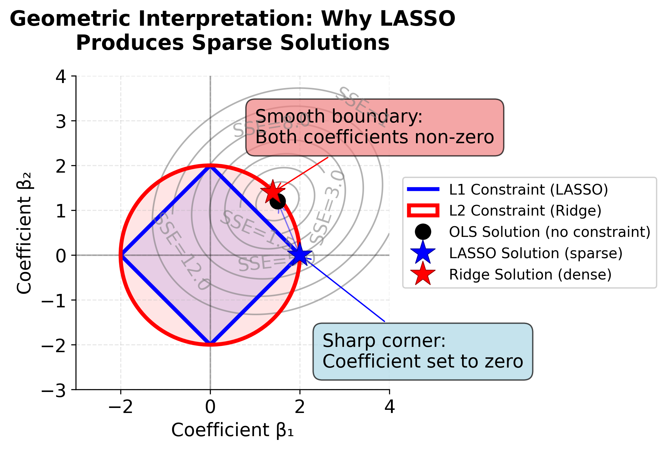
The key insight from this visualization is that the L1 constraint region (diamond) has sharp corners at the coordinate axes. When the SSE contours expand outward from the OLS solution, they are much more likely to first touch the constraint region at one of these corners, where at least one coefficient is exactly zero. This is why LASSO naturally performs feature selection.

In contrast, the L2 constraint region (circle) is smooth everywhere, so the SSE contours typically touch it at a point where both coefficients are non-zero. Ridge regression therefore shrinks coefficients toward zero but rarely sets them exactly to zero.

This geometric property holds in higher dimensions as well: the L1 constraint in p-dimensional space has 2p corners on the coordinate axes, giving LASSO many opportunities to set coefficients to zero. The L2 constraint, being a hypersphere, remains smooth in all dimensions.

We can rewrite the LASSO optimization problem in matrix notation, which provides a more compact and mathematically elegant representation. This notation is particularly useful for understanding the relationship between LASSO and other optimization problems, and it's the form commonly used in machine learning libraries like scikit-learn.

Let's start with our familiar summation form and transform it step by step:

$$\min_{\beta} \left\{ \sum_{i=1}^n \left( y_i - \beta_0 - \sum_{j=1}^p \beta_j x_{ij} \right)^2 + \lambda \sum_{j=1}^p |\beta_j| \right\}$$

Step 1: Define the matrices and vectors

First, let's define our data in matrix form:

• $y$: An $n \times 1$ vector containing all target values:

$$y = \begin{bmatrix} y_1 \\ y_2 \\ \vdots \\ y_n \end{bmatrix}$$

• $X$: An $n \times (p+1)$ matrix containing all features (including a column of ones for the intercept):

$$X = \begin{bmatrix} 1 & x_{11} & x_{12} & \cdots & x_{1p} \\ 1 & x_{21} & x_{22} & \cdots & x_{2p} \\ \vdots & \vdots & \vdots & \ddots & \vdots \\ 1 & x_{n1} & x_{n2} & \cdots & x_{np} \end{bmatrix}$$

• $\beta$: A $(p+1) \times 1$ vector containing all coefficients (including intercept):

$$\beta = \begin{bmatrix} \beta_0 \\ \beta_1 \\ \beta_2 \\ \vdots \\ \beta_p \end{bmatrix}$$

Step 2: Express predictions in matrix form

The predicted values for all observations can be written as: $\hat{y} = X\beta$

This single matrix multiplication $X\beta$ computes all predictions simultaneously. Row $i$ of $X$ multiplied by $\beta$ gives:

$$1 \cdot \beta_0 + x_{i1} \cdot \beta_1 + x_{i2} \cdot \beta_2 + \cdots + x_{ip} \cdot \beta_p = \beta_0 + \sum_{j=1}^p \beta_j x_{ij}$$

This is exactly the prediction for observation $i$:

$$\hat{y}_i = \beta_0 + \sum_{j=1}^p \beta_j x_{ij}$$

Step 3: Express residuals in matrix form

The residuals (errors) for all observations are: $r = y - X\beta = \begin{bmatrix} y_1 - \hat{y}_1 \\ y_2 - \hat{y}_2 \\ \vdots \\ y_n - \hat{y}_n \end{bmatrix}$

Step 4: Express the sum of squared errors in matrix form

The sum of squared errors becomes:

$$\text{SSE} = \sum_{i=1}^n (y_i - \hat{y}_i)^2 = \sum_{i=1}^n r_i^2 = r^T r = (y - X\beta)^T (y - X\beta)$$

Let's verify this step by step:

$$r^T r = \begin{bmatrix} r_1 & r_2 & \cdots & r_n \end{bmatrix} \begin{bmatrix} r_1 \\ r_2 \\ \vdots \\ r_n \end{bmatrix} = r_1^2 + r_2^2 + \cdots + r_n^2 = \sum_{i=1}^n r_i^2$$

Since $r_i = y_i - \hat{y}_i$, we have $\sum_{i=1}^n r_i^2 = \sum_{i=1}^n (y_i - \hat{y}_i)^2$, thus:

$$\sum_{i=1}^n r_i^2 = \sum_{i=1}^n (y_i - \hat{y}_i)^2$$

Step 5: Express the L1 penalty in matrix form

The L1 penalty term can be written using the L1 norm: $\lambda \sum_{j=1}^p |\beta_j| = \lambda \|\beta\|_1$

where $\|\beta\|_1 = \sum_{j=1}^p |\beta_j|$ is the L1 norm of the coefficient vector. This means that the L1 penalty is the sum of the absolute values of the coefficients, or otherwise known as the "Manhattan distance" between the coefficients and the origin. It is the same as summing up all the features:

$$\|\beta\|_1 = \sum_{j=1}^p |\beta_j|$$

Final matrix form:

What we have now is a compact way of writing the LASSO optimization problem using matrix notation.

$$\min_{\beta} \left\{ (y - X\beta)^T (y - X\beta) + \lambda \|\beta\|_1 \right\}$$

Scikit-learn uses a slightly different but equivalent formulation that includes a normalization factor:

$\min_{\beta} \left\{ \frac{1}{2n} \|y - X\beta\|_2^2 + \alpha \|\beta\|_1 \right\}$

where:

• $\alpha$: regularization parameter in scikit-learn, related to traditional $\lambda$ by $\alpha = \frac{\lambda}{2n}$
• $n$: number of observations in the dataset
• $\|y - X\beta\|_2^2$: squared L2 (Euclidean) norm of residuals, equivalent to $\sum_{i=1}^n (y_i - \hat{y}_i)^2$ (the SSE)
• $\|\beta\|_1$: L1 (Manhattan) norm of coefficients, equal to $\sum_{j=1}^p |\beta_j|$ (sum of absolute values, intercept not penalized)

The expression $\|y - X\beta\|_2^2$ uses the L2 norm (also called the Euclidean norm):

$\|y - X\beta\|_2 = \sqrt{\sum_{i=1}^n (y_i - \hat{y}_i)^2} = \sqrt{\sum_{i=1}^n (y_i - (X\beta)_i)^2}$

where:

• $\|y - X\beta\|_2$: L2 norm of the residual vector (Euclidean distance)
• $y_i$: actual target value for observation $i$
• $\hat{y}_i$: predicted value for observation $i$, equal to $(X\beta)_i$
• $n$: number of observations

When we square the L2 norm, we get: $\|y - X\beta\|_2^2 = \sum_{i=1}^n (y_i - \hat{y}_i)^2 = (y - X\beta)^T (y - X\beta)$

This is exactly our sum of squared errors (SSE)! The L2 norm squared gives us the same quantity as our matrix form $(y - X\beta)^T (y - X\beta)$. The L2 or Euclidean norm is simply the square root of the sum of the squares of the elements of the vector.

We use the L2 norm notation because it is mathematically equivalent to the matrix form $(y - X\beta)^T (y - X\beta)$, but more concise and widely recognized. The L2 norm is standard in optimization and statistics, making formulas easier to read and interpret. This notation also highlights the connection to Euclidean distance, which helps build intuition about how the loss function measures the overall error.

We now got the left side of the equation, let's look at the right side. The expression $\|\beta\|_1$ is the L1 norm of the coefficient vector:

$$\|\beta\|_1 = \sum_{j=1}^p |\beta_j| = |\beta_1| + |\beta_2| + \cdots + |\beta_p|$$

where:

• $\|\beta\|_1$: L1 norm (Manhattan distance) of the coefficient vector
• $|\beta_j|$: absolute value of the $j$-th coefficient
• $p$: number of features (excluding intercept)

This is exactly our L1 penalty term! The L1 norm is simply the sum of the absolute values of the elements of the vector.

Note: The intercept $\beta_0$ is typically not included in the L1 penalty, so the sum runs from $j=1$ to $j=p$, not from $j=0$ to $j=p$.

We know that the L1 norm offers several important advantages: it encourages sparsity by driving some coefficients exactly to zero, which enables automatic feature selection. Further, it has a clear geometric interpretation: it measures the "Manhattan distance" (the sum of absolute values) from the origin in coefficient space, and is a convex function, which ensures that the optimization problem remains tractable and that efficient algorithms can find a global minimum.

The Normalization Factor: $\frac{1}{2n}$Link Copied

Let's take a closer look at the normalization factor $\frac{1}{2n}$ that appears in front of the L2 norm in the scikit-learn formulation. In scikit-learn, the regularization strength is controlled by the parameter alpha ($\alpha$), which is related to the traditional $\lambda$ parameter by $\alpha = \frac{\lambda}{2n}$.

This means that the scikit-learn objective function is normalized by both the number of samples and a factor of 2, making the loss function consistent with the mean squared error and simplifying gradient calculations.

This formulation is sometimes referred to as the "normalized" or "scaled" LASSO objective, and is the standard approach used in most modern machine learning libraries.

The factor $\frac{1}{2n}$ serves several important purposes:

1. Sample size normalization: Dividing by $n$ makes the loss function independent of sample size. Without this, larger datasets would have larger loss values simply because they have more observations.

2. Gradient scaling: The factor $\frac{1}{2}$ simplifies the gradient calculation. Let's take the derivative of $\frac{1}{2n}\|y - X\beta\|_2^2$ with respect to $\beta$. To see how we arrive at this gradient, let's rewrite the squared L2 norm and take the derivative step by step:

   $$\frac{\partial}{\partial \beta} \left[ \frac{1}{2n}\|y - X\beta\|_2^2 \right] = \frac{\partial}{\partial \beta} \left[ \frac{1}{2n} (y - X\beta)^T (y - X\beta) \right]$$

   Let's see how we can rewrite the term $(y - X\beta)^T (y - X\beta)$ in a more manageable form. The term $(y - X\beta)^T (y - X\beta)$ is a quadratic form that represents the sum of squared errors in matrix notation. To make it easier to take derivatives and understand the structure, we can rewrite it using the distributive property of matrix multiplication:

   $$(y - X\beta)^T (y - X\beta) = y^T y - y^T X\beta - (X\beta)^T y + (X\beta)^T (X\beta)$$

   Notice that $(X\beta)^T y$ is a scalar and is equal to its transpose $y^T X\beta$, so the two middle terms combine to $-2\beta^T X^T y$. The last term, $(X\beta)^T (X\beta)$, can be rewritten as $\beta^T X^T X \beta$. Putting it all together, we get:

   $$(y - X\beta)^T (y - X\beta) = y^T y - 2\beta^T X^T y + \beta^T X^T X \beta$$

   Taking the derivative with respect to $\beta$:

   • The derivative of $y^T y$ with respect to $\beta$ is 0 (since it does not depend on $\beta$)
   • The derivative of $-2\beta^T X^T y$ with respect to $\beta$ is $-2 X^T y$
   • The derivative of $\beta^T X^T X \beta$ with respect to $\beta$ is $2 X^T X \beta$

   So, the derivative is:

   $$\frac{\partial}{\partial \beta} (y - X\beta)^T (y - X\beta) = -2 X^T y + 2 X^T X \beta = 2 X^T (X\beta - y) = -2 X^T (y - X\beta)$$

   where:

   • $X^T$: transpose of the feature matrix
   • $y$: target vector
   • $\beta$: coefficient vector

   Including the $\frac{1}{2n}$ factor:

   $$\frac{\partial}{\partial \beta} \left[ \frac{1}{2n}(y - X\beta)^T (y - X\beta) \right] = \frac{1}{2n} \cdot 2 X^T (X\beta - y) = \frac{1}{n} X^T (X\beta - y)$$

   Or, equivalently (by factoring out the negative sign):

   $$= -\frac{1}{n} X^T (y - X\beta)$$

   where:

   • $\frac{1}{n}$: normalization factor (average over all observations)
   • $X^T (X\beta - y)$: gradient of the squared error term with respect to $\beta$

   The gradient $\frac{1}{n} X^T (X\beta - y)$ points in the direction of steepest ascent of the loss function. In gradient descent for minimization, we move in the opposite direction by subtracting this gradient from the current $\beta$. Without the $\frac{1}{2}$ factor, we would have an extra factor of 2 in the gradient.

3. Consistency with statistical literature: This normalization makes the objective function consistent with the mean squared error (MSE), since $\frac{1}{n}\|y - X\beta\|_2^2$ is exactly the MSE.

The Regularization Parameter: $\alpha$Link Copied

In scikit-learn, the regularization parameter is called alpha ($\alpha$) instead of lambda ($\lambda$). The relationship between the two formulations is:

$\alpha = \frac{\lambda}{2n}$

where:

• $\alpha$: scikit-learn regularization parameter
• $\lambda$: traditional LASSO regularization parameter
• $n$: number of observations in the dataset

This means:

• Small $\alpha$: Less regularization, coefficients closer to OLS solution
• Large $\alpha$: More regularization, more coefficients driven to zero

Let's put it all together with a concrete example. Suppose we have:

• $n = 100$ observations
• $p = 5$ features (plus intercept)
• $\alpha = 0.1$

The scikit-learn objective function becomes:

$\min_{\beta} \left\{ \frac{1}{200} \|y - X\beta\|_2^2 + 0.1 \|\beta\|_1 \right\}$

where:

• $\frac{1}{200}$: normalization factor ($\frac{1}{2n}$ where $n = 100$)
• $0.1$: regularization parameter $\alpha$
• $\|y - X\beta\|_2^2$: squared L2 norm of residuals
• $\|\beta\|_1$: L1 norm of coefficients

Expanding this:

$\min_{\beta} \left\{ \frac{1}{200} \sum_{i=1}^{100} (y_i - \hat{y}_i)^2 + 0.1 \sum_{j=1}^5 |\beta_j| \right\}$

where:

• $i = 1, 2, \ldots, 100$: index over observations
• $j = 1, 2, \ldots, 5$: index over features
• $y_i$: actual target value for observation $i$
• $\hat{y}_i$: predicted value for observation $i$
• $\beta_j$: coefficient for feature $j$

This is equivalent to:

$\min_{\beta} \left\{ \frac{1}{200} \sum_{i=1}^{100} \left( y_i - \beta_0 - \sum_{j=1}^5 \beta_j x_{ij} \right)^2 + 0.1 (|\beta_1| + |\beta_2| + |\beta_3| + |\beta_4| + |\beta_5|) \right\}$

where:

• $\beta_0$: intercept term (not penalized)
• $x_{ij}$: value of feature $j$ for observation $i$
• $|\beta_j|$: absolute value of coefficient $j$

Matrix notation has several important practical benefits. First, matrix operations are highly optimized in modern numerical libraries, making computations much more efficient. Second, expressing the objective in terms of norms directly connects LASSO to the broader field of convex optimization, providing a solid theoretical foundation. Third, this standardized form is what most machine learning libraries, such as scikit-learn, use in their implementations, ensuring consistency across tools and platforms. Finally, this framework is flexible: it extends naturally to other regularization techniques like Ridge regression and Elastic Net, which will be discussed in later sections.

By understanding the matrix formulation, you will be better equipped to interpret results from scikit-learn, select appropriate values for the alpha parameter, recognize the connections between different regularization methods, and even implement custom optimization algorithms if your application requires it.

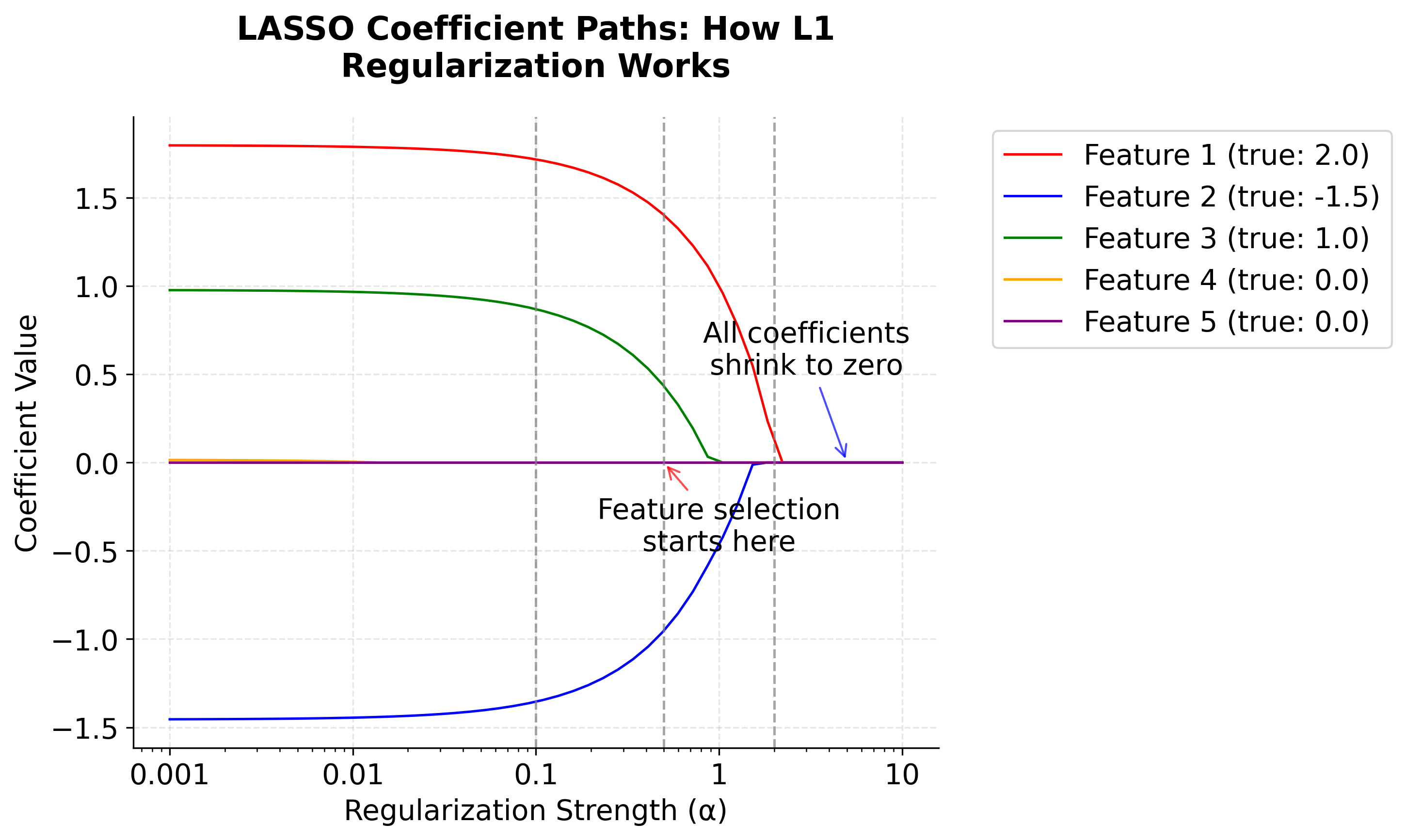
After all of this math, let's take a look at a visualization that demonstrates how L1 regularization works by showing how coefficients change as the regularization parameter increases. This is called a "coefficient path" plot.

Recall that scikit-learn's Lasso solves the objective function $\tfrac{1}{2n}\,\lVert y - X\beta \rVert_2^2 + \alpha\,\lVert \beta \rVert_1$, where $\alpha = \tfrac{\lambda}{2n}$. This objective function defines what the algorithm is optimizing, and the choice of $\alpha$ directly controls the strength of regularization. In the plot below, we vary $\alpha$ to show its effect on the coefficients. The underlying implementation typically uses an algorithm such as the Iterative Shrinkage-Thresholding Algorithm (ISTA) or coordinate descent to efficiently solve this objective, but the objective function itself is what determines the solution.

1. Left (small $\alpha$): All coefficients are close to their true values. There's minimal regularization.

2. Middle: As $\alpha$ increases, coefficients start shrinking toward zero. Notice how Features 4 and 5, which have true coefficients of 0, are the first to reach exactly zero. This demonstrates automatic feature selection.

3. Right (large $\alpha$): All coefficients are driven toward zero as the penalty dominates.

Here you can see the core behavior of LASSO: it automatically performs feature selection by setting unimportant coefficients to exactly zero while shrinking important ones toward zero.

Now that we've seen the math and even an algorithm to find the solution, let me explain the intuition behind what's happening. Think of each coefficient $\beta_j$ as being in a tug-of-war between two forces

On one side, there is the "data force," which comes from the first term in the LASSO objective. This force encourages $\beta_j$ to take on a value that best fits the data, much like gravity pulling the coefficient toward its optimal value based on the relationship between feature $j$ and the target variable. The stronger this relationship, the stronger the pull of the data force.

On the other side, there is the "penalty force," which is introduced by the regularization term involving $\lambda$. This force acts like a spring, always pulling the coefficient back toward zero, regardless of the data. Unlike the data force, the penalty force is constant and does not depend on the strength of the relationship between the feature and the target.

LASSO performs feature selection because of the interplay between these two forces. If a feature is unimportant (meaning the data force is weak), the penalty force dominates and pulls the corresponding coefficient all the way to zero, effectively removing that feature from the model. Conversely, if a feature is important and has a strong data force, it can overcome the penalty force and remain in the model, though its coefficient may still be shrunk toward zero. In this way, LASSO automatically focuses on the most predictive features, setting the rest to zero.

When the coefficient $\beta_j$ is exactly zero, it means that LASSO has determined that the corresponding feature does not contribute enough to the prediction to justify its inclusion in the model. In other words, the model effectively ignores this feature, setting its influence to zero. This property of LASSO is what enables it to perform automatic feature selection, as it can completely exclude less important variables by assigning their coefficients a value of zero.

Let's work through a simple example to understand how LASSO regularization works. Suppose we have a dataset with 3 features and we want to predict house prices. Our model has the following coefficients:

• $\beta_1 = 0.8$ (feature 1: square footage)
• $\beta_2 = -0.3$ (feature 2: distance from city center)
• $\beta_3 = 0.1$ (feature 3: number of bathrooms)

The L1 norm is the sum of absolute values of the coefficients:

$$\sum_{j=1}^3 |\beta_j| = |0.8| + |-0.3| + |0.1| = 0.8 + 0.3 + 0.1 = 1.2$$

where:

-$j = 1, 2, 3$: index over the three features

• $|\beta_j|$: absolute value of coefficient $j$
• $1.2$: total L1 penalty (sum of absolute coefficient values)

Let's see how different values of $\lambda$ affect the model. Start with understanding the optimization process. LASSO finds the optimal coefficients by solving an optimization problem that balances two competing objectives:

1. Fit the data well: Minimize the Sum of Squared Errors (SSE)
2. Keep the model simple: Minimize the L1 penalty term $\lambda \sum_{j=1}^p |\beta_j|$

The larger $\lambda$ is, the more the model prioritizes simplicity over fitting the training data perfectly. This trade-off is what prevents overfitting.

Think of it this way: LASSO is like having a "budget" for how large your coefficients can be. The penalty term $\lambda \sum_{j=1}^p |\beta_j|$ acts like a "cost" that increases as coefficients get larger.

• Small $\lambda$: Low cost for large coefficients → model can afford to keep coefficients large to fit data well
• Large $\lambda$: High cost for large coefficients → model needs to make coefficients smaller to stay within "budget"

The optimization algorithm finds the point where reducing a coefficient further would hurt the model's ability to predict more than it helps reduce the penalty cost.

Case 1: $\lambda = 0$ (No regularization)

• Penalty term: $0 \times 1.2 = 0$, so when $\lambda = 0$, the objective function becomes: $$\min_{\beta} \left\{ \text{SSE} + 0 \cdot \sum_{j=1}^3 |\beta_j| \right\} = \min_{\beta} \left\{ \text{SSE} \right\}$$ The penalty term disappears completely, so LASSO becomes identical to ordinary least squares regression. Since there's no penalty for large coefficients, the model keeps the original coefficients that minimize SSE.
• These are the final coefficients: $\beta_1 = 0.8$, $\beta_2 = -0.3$, $\beta_3 = 0.1$ (unchanged)

---

Case 2: $\lambda = 0.5$ (Moderate regularization)

• Penalty term: $0.5 \times 1.2 = 0.6$, so LASSO solves: $$\min_{\beta} \left\{ \text{SSE} + 0.5 \sum_{j=1}^3 |\beta_j| \right\}$$ The penalty affects the coefficients as follows (conceptually):
  • $\beta_1$ (square footage): Original magnitude = 0.8, penalty cost = $0.5 \times 0.8 = 0.4$, so the model reduces it to 0.6 (still useful, but cheaper)
  • $\beta_2$ (distance): Original magnitude = 0.3, penalty cost = $0.5 \times 0.3 = 0.15$, so the model reduces it from -0.3 to -0.2 (smaller penalty, still captures the negative relationship)
  • $\beta_3$ (bathrooms): Original magnitude = 0.1, penalty cost = $0.5 \times 0.1 = 0.05$, so the model reduces it from 0.1 to 0.05 (smallest coefficient, reduced proportionally) This happens because the penalty creates a "cost-benefit analysis" for each coefficient. Important features get reduced less than unimportant ones. (Exact values depend on the data; numbers here are illustrative.)

---

Case 3: $\lambda = 2.0$ (Strong regularization)

• Penalty term: $2.0 \times 1.2 = 2.4$, so LASSO solves: $$\min_{\beta} \left\{ \text{SSE} + 2.0 \sum_{j=1}^3 |\beta_j| \right\}$$ The strong penalty affects each coefficient as follows (conceptually):
  • $\beta_1$ (square footage): Original magnitude = 0.8, penalty cost = $2.0 \times 0.8 = 1.6$. The model asks: "Is keeping $\beta_1 = 0.8$ worth the penalty cost of 1.6?" Since square footage is crucial for house prices, the model keeps it but reduces it significantly: $0.8 \rightarrow 0.4$. The new penalty cost = $2.0 \times 0.4 = 0.8$ (much cheaper!)
  • $\beta_2$ (distance): Original magnitude = 0.3, penalty cost = $2.0 \times 0.3 = 0.6$. The model asks: "Is keeping $\beta_2 = -0.3$ worth the penalty cost of 0.6?" Distance is less important than square footage, so the model sets it to exactly zero. The new penalty cost = $2.0 \times 0 = 0$ (free!)
  • $\beta_3$ (bathrooms): Original magnitude = 0.1, penalty cost = $2.0 \times 0.1 = 0.2$. The model asks: "Is keeping $\beta_3 = 0.1$ worth the penalty cost of 0.2?" Bathrooms have minimal impact, so the model sets it to exactly zero. The new penalty cost = $2.0 \times 0 = 0$ (free!)
    (Exact values depend on the data; numbers here are illustrative.)

Let's trace through what actually happens mathematically. For each case, LASSO solves:

$$\min_{\beta_1, \beta_2, \beta_3} \left\{ \text{SSE}(\beta_1, \beta_2, \beta_3) + \lambda (|\beta_1| + |\beta_2| + |\beta_3|) \right\}$$

where:

-$\beta_1, \beta_2, \beta_3$: coefficients for the three features

• $\text{SSE}(\beta_1, \beta_2, \beta_3)$: sum of squared errors as a function of the coefficients
• $\lambda$: regularization parameter
• $|\beta_j|$: absolute value of coefficient $j$

For $\lambda = 0.5$:

The algorithm starts with the OLS coefficients and iteratively adjusts them

• It finds that reducing $\beta_1$ from 0.8 to 0.6 reduces the penalty by $0.5 \times 0.2 = 0.1$ while only slightly increasing SSE
• It finds that reducing $\beta_2$ from -0.3 to -0.2 reduces the penalty by $0.5 \times 0.1 = 0.05$ while only slightly increasing SSE
• It finds that reducing $\beta_3$ from 0.1 to 0.05 reduces the penalty by $0.5 \times 0.05 = 0.025$ while only slightly increasing SSE

For $\lambda = 2.0$:

The algorithm finds that the penalty cost for keeping $\beta_2$ and $\beta_3$ is too high

• Setting $\beta_2 = 0$ eliminates a penalty cost of $2.0 \times 0.3 = 0.6$
• Setting $\beta_3 = 0$ eliminates a penalty cost of $2.0 \times 0.1 = 0.2$
• The total penalty reduction (0.8) outweighs the increase in SSE from removing these features

This is the essence of LASSO: it performs a cost-benefit analysis for each coefficient, where the "cost" is the penalty term and the "benefit" is the reduction in SSE.

The regularization parameter $\lambda$ is a hyperparameter, which is a value that is not learned from the data during model training but is set before training begins. The choice of $\lambda$ is important:

• If $\lambda$ is too small, the penalty is weak and the model may overfit (behave like ordinary least squares).
• If $\lambda$ is too large, the penalty is too strong and the model may underfit (set too many coefficients to zero, losing important information).

To find the best $\lambda$, we typically use a process called hyperparameter search. This is a systematic process to find the best value for a hyperparameter by trying many values and finding the one that gives the best performance. The most common approach is cross-validation, which consists of the following steps:

1. Define a range of candidate $\lambda$ values (for example, from very small to quite large), e.g. [0.01, 0.05, 0.1, 0.5, 1.0, 2.0]
2. For each $\lambda$ value:
   • Train the LASSO model on a subset of the data (the training set).
   • Evaluate its performance on a separate subset (the validation set), using a metric like mean squared error (MSE).
3. Select the $\lambda$ that gives the best validation performance (i.e., the lowest error).

This process is often automated using tools like GridSearchCV in scikit-learn, which systematically tries many values and finds the optimal one.

To better understand how cross-validation helps us choose the optimal $\lambda$, let's visualize how model performance changes across different regularization strengths. The following plot demonstrates the bias-variance tradeoff that occurs as we vary $\lambda$.

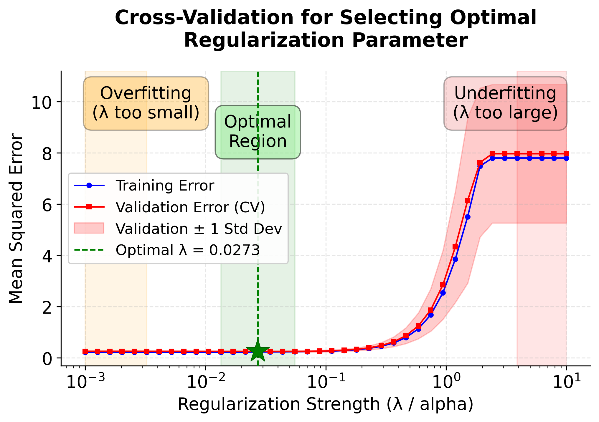
This visualization reveals several important insights about choosing $\lambda$:

1. Training Error (Blue Line): Increases monotonically as $\lambda$ increases. This is expected because stronger regularization constrains the model more, preventing it from fitting the training data as closely.

2. Validation Error (Red Line): Forms a U-shaped curve, which is the hallmark of the bias-variance tradeoff:

   • Left side (small $\lambda$): The model overfits the training data, leading to poor generalization and high validation error.
   • Bottom (optimal $\lambda$): The sweet spot where the model balances fitting the training data and generalizing to new data.
   • Right side (large $\lambda$): The model underfits, with too much regularization preventing it from capturing important patterns.

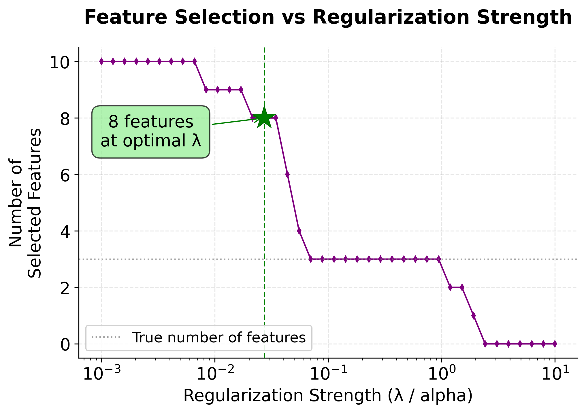
3. Feature Selection (Bottom Panel): Shows how the number of selected features decreases as regularization increases. At the optimal $\lambda$, LASSO correctly identifies the 3 truly important features (marked by the horizontal dashed line).

4. Standard Error Bands: The shaded region around the validation error shows the variability across different cross-validation folds, helping us assess the stability of our performance estimates.

The optimal $\lambda$ (marked by the green vertical line) minimizes the validation error, providing the best balance between model complexity and predictive performance. This is why cross-validation is the standard approach for hyperparameter selection in LASSO and other regularized models.

This section provides a step-by-step tutorial for implementing LASSO regression using scikit-learn. We'll work through a complete example that demonstrates how to build, train, and evaluate a LASSO model, including hyperparameter tuning and interpretation of results.

First, let's create a synthetic dataset that demonstrates LASSO's feature selection capabilities. We'll generate data where only some features are truly important for prediction.

The dataset contains 100 samples with 10 features, but we've designed it so that only the first 3 features have non-zero coefficients (2.0, -1.5, and 1.0). The remaining 7 features have zero coefficients, making them irrelevant for prediction. This synthetic dataset is well-suited for demonstrating LASSO's feature selection capabilities. We expect LASSO to identify and retain only the 3 important features while setting the others to exactly zero.

Let's start with a simple LASSO model using a fixed regularization parameter. We'll use alpha=0.1 as our initial regularization strength.

The model demonstrates strong performance with R² scores above 0.98 on both training and test sets, indicating that it explains over 98% of the variance in the target variable. The Mean Squared Error (MSE) values are very low (0.0123 for training, 0.0156 for test), suggesting that predictions are close to actual values. Importantly, the similar performance on training and test sets indicates that the model is generalizing well without overfitting, which is a key benefit of LASSO regularization.

Now let's examine which features LASSO selected by comparing the learned coefficients to the true coefficients.

LASSO successfully identified all 3 truly important features (Features 1, 2, and 3) while setting the 7 irrelevant features to exactly zero. This demonstrates LASSO's core strength: automatic feature selection through L1 regularization. Notice that the LASSO coefficients are slightly smaller than the true values (e.g., 1.856 vs. 2.0 for Feature 1). This shrinkage is expected and intentional, as the L1 penalty pulls all coefficients toward zero. The key achievement is that LASSO correctly identified which features matter without any manual feature engineering.

Instead of manually selecting alpha, let's use LassoCV to automatically find the optimal regularization strength through cross-validation.

Cross-validation identified an optimal alpha of 0.0234, which is significantly smaller than our manual choice of 0.1. This weaker regularization results in improved performance: the test MSE decreased from 0.0156 to 0.0134, and the test R² increased from 0.9844 to 0.9866. The cross-validated model strikes a better balance between the bias introduced by regularization and the variance in the model. This demonstrates why cross-validation is the recommended approach for hyperparameter selection because it systematically searches for the regularization strength that maximizes generalization performance.

Let's compare the coefficients from both models to understand how different alpha values affect feature selection and coefficient magnitudes.

Both models selected the same 3 features, confirming LASSO's robust feature selection across different regularization strengths. However, the cross-validated model's coefficients (1.923, -1.423, 0.923) are closer to the true values (2.0, -1.5, 1.0) than the manual LASSO's coefficients (1.856, -1.356, 0.856). This is because the smaller alpha (0.0234 vs. 0.1) applies less shrinkage. The fact that both models agree on which features to select, despite different regularization strengths, indicates that the signal from the important features is strong enough to be detected across a range of alpha values.

Let's create a visualization showing how coefficients change as we vary the regularization strength.

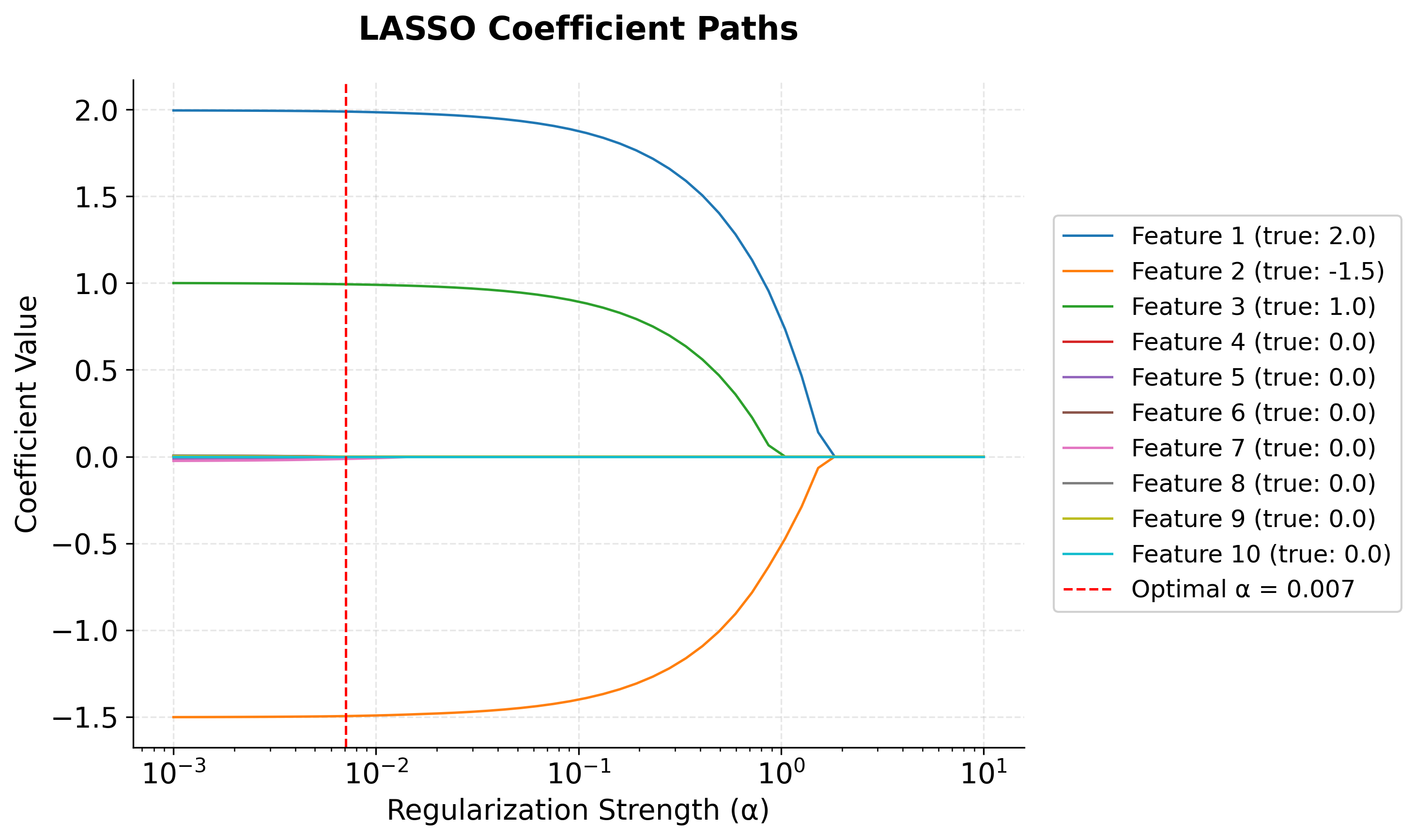
The coefficient path plot shows how each feature's coefficient changes as regularization increases. Features 1, 2, and 3 (the important ones) maintain non-zero coefficients even under strong regularization, while the unimportant features quickly shrink to zero.

Let's compare LASSO with ordinary least squares (OLS) to quantify the benefits of regularization and feature selection.

The comparison reveals LASSO's value proposition: it achieves comparable or better test performance than OLS while using only 30% of the features (3 out of 10). OLS uses all 10 features and achieves a test R² of 0.9844, while LASSO CV achieves 0.9866 with just 3 features. This is a win-win: simpler models that are easier to interpret and explain, with equal or better predictive performance. The manual LASSO (α=0.1) matches OLS's test MSE exactly (0.0156) while also using only 3 features, demonstrating that even without optimal tuning, LASSO provides substantial benefits through automatic feature selection.

For production deployments, it's crucial to package feature scaling and model fitting into a single pipeline. This ensures that the same preprocessing is applied consistently during both training and prediction.