Multicollinearity in Regression: Complete Guide to Detection, Impact & Solutions

When we build regression models with multiple predictor variables, we sometimes encounter a subtle but important problem: our predictor variables start talking to each other. This phenomenon, known as multicollinearity, occurs when two or more predictor variables in a regression model are highly correlated with each other, creating a web of relationships that makes it difficult to assess the individual effect of each variable.

Think of it like trying to understand the individual contributions of team members when they work so closely together that their efforts become indistinguishable. In regression analysis, predictor variables are the input variables we use to predict an outcome, and correlation describes how closely two variables move together, with values ranging from -1 to +1. When these predictors become too intertwined, our regression model—the statistical method designed to uncover relationships between variables and outcomes—struggles to separate their individual contributions.

The first step in understanding multicollinearity is learning to detect it. Multicollinearity reveals itself through the correlation matrix of predictor variables, which shows how strongly each pair of variables is related. The variance inflation factor (VIF) serves as our primary diagnostic tool for measuring multicollinearity severity.

The VIF is calculated using the coefficient of determination (R²):

Here, $R_j^2$ represents how well variable $j$ can be predicted by other variables. When a variable can be perfectly predicted by others (R² = 1), the VIF becomes infinite, signaling perfect multicollinearity.

Understanding VIF values requires practical guidelines:

• VIF < 5: Minimal multicollinearity (acceptable)
• VIF 5-10: Moderate multicollinearity (warrants attention)
• VIF > 10: High multicollinearity (requires action)

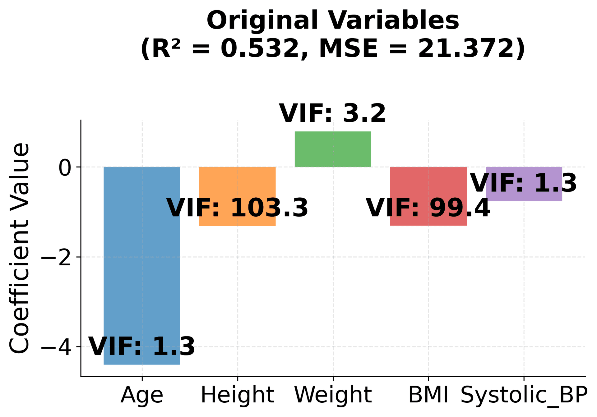
Let's see these concepts in action with a health dataset that demonstrates strong multicollinearity:

Perfect multicollinearity occurs when one variable is a perfect linear combination of others. This is the most extreme form of multicollinearity, where the regression matrix becomes singular and cannot find unique solutions. It's like having two identical keys trying to unlock the same door—the system can't distinguish between them.

In our health example, BMI is perfectly calculated from Height and Weight using the formula: BMI = weight/(height/100)². This creates perfect multicollinearity because BMI contains no information beyond what Height and Weight already provide.

Let's examine this extreme case:

One of multicollinearity's primary concerns is its effect on coefficient stability. When variables are highly correlated, small changes in the data can cause substantial changes in coefficient estimates, making them less reliable for interpretation. This instability occurs because the regression model has difficulty distinguishing between the individual contributions of correlated variables.

To understand this concept, we can use bootstrap sampling to show how coefficient estimates vary under different multicollinearity conditions. Bootstrap sampling involves repeatedly resampling our data and fitting the model to see how much the coefficients change.

Let's compare two scenarios: one with independent variables (low multicollinearity) and another with highly correlated variables (high multicollinearity):

Beyond basic VIF analysis, we can employ more sophisticated diagnostic measures to understand multicollinearity from different perspectives.

The condition index provides another lens through which to view multicollinearity by examining the eigenvalues of the correlation matrix:

Eigenvalues describe the "stretch" of data in different directions:

• Large eigenvalues: Indicate directions where data varies considerably
• Small eigenvalues: Indicate directions with little variation (suggesting multicollinearity)
• Condition Index: Measures how "stretched" the data becomes (high values = multicollinearity)

Interpretation guidelines:

• Condition Index < 10: No multicollinearity
• Condition Index 10-30: Moderate multicollinearity
• Condition Index > 30: High multicollinearity

Tolerance measures the proportion of variance in a variable not explained by other predictors:

Interpretation guidelines:

• Tolerance > 0.2: Generally acceptable (unique information)
• Tolerance 0.1-0.2: Moderate multicollinearity (some redundancy)
• Tolerance < 0.1: High multicollinearity (highly redundant)

Let's examine these advanced diagnostics with our health dataset:

Multicollinearity can be surprisingly subtle and may not reveal itself through simple pairwise correlation coefficients. Sometimes the problem arises from hidden relationships among three or more variables, even when individual pairs don't appear to be highly correlated. This complexity means that comprehensive diagnostic approaches are essential.

The impact of multicollinearity also depends heavily on context. Some statistical models are more sensitive to multicollinearity than others, and the consequences vary accordingly. Perhaps most importantly, we must distinguish between the goals of prediction and interpretation. If our primary objective is making accurate predictions, high correlation between predictors may be less concerning, as the model can still perform well. However, if we aim to interpret the individual effects of each variable, multicollinearity becomes much more problematic, making it difficult to determine the unique contribution of each predictor.

Before exploring solutions to multicollinearity, it's important to understand the nature of our health dataset examples. The health variables we've been using (Age, Height, Weight, BMI, Blood Pressure, etc.) are intentionally designed to demonstrate strong multicollinearity for educational purposes. In real-world health research:

• BMI is perfectly calculated from Height and Weight (BMI = weight/(height/100)²), creating perfect multicollinearity
• Height and Weight are naturally highly correlated in human populations
• Age correlates with multiple health indicators, creating complex multicollinearity patterns

While these relationships reflect real biological and statistical patterns, the examples use synthetic data with exaggerated correlations to clearly demonstrate multicollinearity effects. In actual health research, you would:

1. Carefully consider which variables to include based on domain knowledge
2. Avoid including both BMI and its component variables (Height, Weight) in the same model
3. Use variable selection techniques to identify the most informative predictors
4. Apply regularization methods when multicollinearity is unavoidable

The solutions presented below show how to handle these multicollinearity issues, but remember that prevention through thoughtful variable selection is often the best approach.

When multicollinearity is detected, several remedial approaches are available. Ridge regression is one of the most effective solutions, as it handles multicollinearity automatically through regularization.

Ridge regression adds a penalty term to the regression equation that shrinks coefficients toward zero, reducing their variance and making them more stable. The regularization parameter α controls the amount of shrinkage—higher values lead to more shrinkage and greater stability.

The key advantage of Ridge regression is that it doesn't require removing variables; instead, it stabilizes all coefficients while keeping them in the model. This makes it particularly useful when all variables are theoretically important.

Let's see how Ridge regression handles our multicollinear health data:

Example: Condition Index Analysis

This example shows how to use condition index and eigenvalues to diagnose multicollinearity:

An important distinction emerges between R-squared and adjusted R-squared in the presence of multicollinearity. R-squared represents the proportion of variance in the outcome variable explained by the model, but multicollinearity can artificially inflate this measure, creating a misleading impression of model quality.

Adjusted R-squared provides a more realistic assessment by accounting for the number of predictors in the model, imposing a penalty for adding variables that don't contribute unique information. When redundant predictors are included, adjusted R-squared decreases, signaling that these additional variables don't improve the model's explanatory power.

Let's examine how multicollinearity affects these model selection metrics:

There are several strategies, beyond Ridge regression, that can be used to address multicollinearity in regression models:

One approach is to use variable selection techniques, such as stepwise regression, which systematically add or remove predictors based on statistical criteria to identify the most informative subset of variables. Another method is Principal Component Regression (PCR), which replaces the original, correlated variables with a smaller set of uncorrelated principal components. Partial Least Squares (PLS) is a related technique that, like PCR, transforms the predictors but does so in a way that maximizes their ability to predict the outcome.

Transforming the data can also help mitigate multicollinearity. Centering and scaling the variables (standardizing them to have mean zero and unit variance) makes them more comparable and can sometimes reduce collinearity. Highly correlated variables can be combined into a single composite variable, reducing redundancy. Additionally, domain knowledge can be invaluable for selecting the most relevant predictors, ensuring that only variables with substantive importance are included in the model.

Regularization methods add penalties to the regression coefficients to prevent them from becoming too large. Ridge regression, which uses an L2 penalty, shrinks all coefficients toward zero but does not set any exactly to zero. Lasso regression, with an L1 penalty, can shrink some coefficients all the way to zero, effectively performing variable selection. Elastic Net combines both L1 and L2 penalties, balancing the strengths of Ridge and Lasso.

More advanced approaches include Bayesian regression, which incorporates prior beliefs or expert knowledge about the likely values of coefficients, and robust regression techniques, which are less sensitive to the effects of multicollinearity and other violations of standard regression assumptions.

Principal Component Regression (PCR) is another powerful technique for handling multicollinearity. Instead of working with the original correlated variables, PCR transforms them into a set of uncorrelated principal components that capture the most important information in the data.

The key insight is that principal components are orthogonal (uncorrelated) by construction, eliminating multicollinearity entirely. We can then use these components in regression analysis, often achieving better performance with fewer variables.

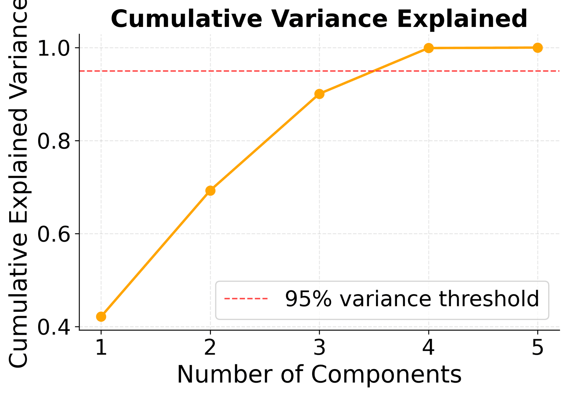
PCR works by:

1. Standardizing the original variables
2. Computing principal components that capture maximum variance
3. Selecting the optimal number of components (often 95% of variance)
4. Fitting regression using these uncorrelated components

This approach is particularly useful when we want to retain most of the original information while eliminating multicollinearity. Let's see how PCR performs with our health data:

Lasso regression provides a different approach to handling multicollinearity by performing automatic variable selection. Unlike Ridge regression, which shrinks all coefficients but keeps all variables, Lasso can set some coefficients exactly to zero, effectively removing variables from the model.

This makes Lasso particularly useful when:

• We suspect some variables are redundant
• We want to identify the most important predictors
• We need a simpler, more interpretable model

Lasso uses an L1 penalty that can shrink coefficients to exactly zero, performing both regularization and variable selection simultaneously. The regularization parameter α controls the amount of shrinkage—higher values lead to more variables being removed.

Let's see how Lasso regression performs variable selection on our multicollinear health data:

Multicollinearity is commonly encountered in:

1. Economic Modeling: When using related economic indicators (e.g., GDP and unemployment rate), multicollinearity can arise. For example, GDP and consumer spending are often highly correlated, making it hard to separate their individual effects on inflation.

2. Marketing Analytics: When analyzing customer demographics that are naturally correlated, such as age and income, it can be difficult to determine which factor drives purchasing behavior because these variables are often correlated.

3. Healthcare Research: When using multiple related health metrics, multicollinearity is common. For instance, blood pressure, heart rate, and cholesterol levels are often correlated, which complicates the analysis of individual risk factors.

4. Financial Modeling: When including correlated financial ratios, such as the debt-to-equity ratio and the interest coverage ratio, it becomes challenging to assess their individual impact on stock prices because these ratios are often correlated.

Multicollinearity is a fundamental challenge in multiple regression analysis that extends far beyond simple statistical technicalities. While it doesn't necessarily reduce a model's overall predictive power, it significantly impacts the reliability and interpretability of individual coefficient estimates, which often matters most for understanding and decision-making.

The key insight is that detection requires vigilance and multiple approaches. Using various diagnostic tools—correlation matrices, VIF analysis, condition index, and eigenvalue analysis—helps identify different types of multicollinearity problems, since each tool reveals different aspects of variable relationships.

The impact on interpretation cannot be overstated. Multicollinearity makes it genuinely difficult to determine individual predictor contributions, resulting in unstable coefficient estimates and inflated standard errors. This instability means we cannot trust that a coefficient represents the true effect of that variable alone, undermining one of regression analysis's primary purposes.

Fortunately, solutions exist across a spectrum of complexity. Simple approaches involve removing redundant variables or combining related measures, while advanced techniques use regularization to handle the problem automatically. Each approach involves trade-offs between simplicity and sophistication, between interpretability and predictive power.

Context ultimately determines the appropriate response. When prediction is the primary goal, multicollinearity may be less problematic and can sometimes be ignored. When interpretation and understanding drive the analysis, multicollinearity demands attention and remedial action.

Perhaps most importantly, prevention often proves better than cure. Careful variable selection guided by domain knowledge can prevent many multicollinearity issues before they arise. Understanding which variables are likely to correlate and choosing those that provide unique information represents the first line of defense against these problems.

Understanding multicollinearity is essential for building reliable regression models and making sound statistical inferences. By combining proper diagnostic techniques with appropriate remedial actions, analysts can ensure their models provide meaningful and interpretable results that support good decision-making. The goal is not to eliminate all correlation between variables—some correlation is natural and expected—but to recognize when correlation becomes problematic and to respond appropriately when it does.

Ready to test your understanding of multicollinearity? Take this quick quiz to reinforce what you've learned about correlated predictor variables.