Simulating stock market returns using Monte Carlo

Michael Brenndoerfer

Data, Analytics & AI Software Engineering Machine Learning

Learn how to use Monte Carlo simulation to model and analyze stock market returns, estimate future performance, and understand the impact of randomness in financial forecasting. This tutorial covers the fundamentals, practical implementation, and interpretation of simulation results.

Reading Level

Toggle tooltip visibility. Hover over underlined terms for instant definitions.

A Simple Yet Complete Tutorial on Estimating Long-Term Investment ReturnsLink Copied

Learning ObjectivesLink Copied

By the end of this tutorial, you will be able to:

Understand the fundamentals of Monte Carlo simulation for financial modeling
Implement a complete investment return simulation using Python
Interpret probability distributions and risk metrics for investment decisions
Create meaningful visualizations to communicate financial uncertainty
Apply these techniques to your own investment analysis

What We'll BuildLink Copied

We'll create a Monte Carlo simulation that estimates the future value of a $100 investment over 10 years, accounting for market volatility and uncertainty. This approach is widely used by financial advisors, portfolio managers, and individual investors to understand potential outcomes and make informed decisions.

Key Concepts CoveredLink Copied

Monte Carlo Method: Using random sampling to model complex systems
Investment Returns: How compound growth works with volatility
Risk Assessment: Understanding percentiles and confidence intervals
Data Visualization: Creating meaningful charts for financial analysis

1. Setting Up The EnvironmentLink Copied

First, let's import the essential libraries we'll need for our simulation and visualization:

In[1]:

import numpy as np
import pandas as pd
import matplotlib.pyplot as plt

# Modern, clean styling
plt.style.use('default')
plt.rcParams.update({
    'figure.facecolor': 'white',
    'axes.facecolor': 'white',
    'axes.edgecolor': '#CCCCCC',
    'axes.linewidth': 0.8,
    'axes.spines.left': True,
    'axes.spines.bottom': True,
    'axes.spines.top': False,
    'axes.spines.right': False,
    'xtick.bottom': True,
    'xtick.top': False,
    'ytick.left': True,
    'ytick.right': False,
    'axes.grid': True,
    'grid.color': '#E5E5E5',
    'grid.linewidth': 0.5,
    'font.size': 11,
    'axes.titlesize': 14,
    'axes.labelsize': 12,
    'figure.dpi': 100
})

import numpy as np
import pandas as pd
import matplotlib.pyplot as plt

# Modern, clean styling
plt.style.use('default')
plt.rcParams.update({
    'figure.facecolor': 'white',
    'axes.facecolor': 'white',
    'axes.edgecolor': '#CCCCCC',
    'axes.linewidth': 0.8,
    'axes.spines.left': True,
    'axes.spines.bottom': True,
    'axes.spines.top': False,
    'axes.spines.right': False,
    'xtick.bottom': True,
    'xtick.top': False,
    'ytick.left': True,
    'ytick.right': False,
    'axes.grid': True,
    'grid.color': '#E5E5E5',
    'grid.linewidth': 0.5,
    'font.size': 11,
    'axes.titlesize': 14,
    'axes.labelsize': 12,
    'figure.dpi': 100
})

2. Defining The Simulation ParametersLink Copied

Understanding the Financial ModelLink Copied

Before diving into the code, let's understand what we're modeling:

Expected Return ( $\mu$ ): The average annual return expected from the investment (8%)
Volatility ( $\sigma$ ): How much the returns vary from year to year (15% standard deviation)
Time Horizon: How long the investment will be held (10 years)
Simulation Paths: How many different scenarios will be tested (10,000 iterations)

Why These Numbers?Link Copied

8% expected return: Roughly matches historical stock market averages
15% volatility: Typical for a diversified stock portfolio
10,000 simulations: Provides statistical confidence in the results

The parameters are defined below:

In[2]:

# Defining parameters for the investment simulation
INITIAL_INVESTMENT = 100.00   
YEARS              = 10       
MU                 = 0.08     # Expected annual return (8%)
SIGMA              = 0.15     # Annual return volatility (15%)
N_ITER             = 10_000   # Number of Monte Carlo simulation paths

print("Investment Simulation Parameters:")
print(f"   Initial Investment: ${INITIAL_INVESTMENT:,.2f}")
print(f"   Time Horizon: {YEARS} years")
print(f"   Expected Annual Return: {MU:.1%}")
print(f"   Annual Volatility: {SIGMA:.1%}")
print(f"   Number of Simulations: {N_ITER:,}")

# Defining parameters for the investment simulation
INITIAL_INVESTMENT = 100.00   
YEARS              = 10       
MU                 = 0.08     # Expected annual return (8%)
SIGMA              = 0.15     # Annual return volatility (15%)
N_ITER             = 10_000   # Number of Monte Carlo simulation paths

print("Investment Simulation Parameters:")
print(f"   Initial Investment: ${INITIAL_INVESTMENT:,.2f}")
print(f"   Time Horizon: {YEARS} years")
print(f"   Expected Annual Return: {MU:.1%}")
print(f"   Annual Volatility: {SIGMA:.1%}")
print(f"   Number of Simulations: {N_ITER:,}")

Out[2]:

Investment Simulation Parameters:
   Initial Investment: $100.00
   Time Horizon: 10 years
   Expected Annual Return: 8.0%
   Annual Volatility: 15.0%
   Number of Simulations: 10,000

3. Generating Random ReturnsLink Copied

The Heart of Monte Carlo SimulationLink Copied

Thousands of possible future scenarios will be generated by randomly sampling investment returns from a normal distribution. This is the core of Monte Carlo simulation:

Key Insight: Annual returns are assumed to follow a normal distribution with:

Mean = 8% (the expected return)
Standard deviation = 15% (market volatility)

Understanding the Output StructureLink Copied

Rows: Each row represents one possible future scenario (simulation path)
Columns: Each column represents a year in the 10-year horizon
Values: Each value is a randomly sampled annual return for that year and scenario

In[3]:

# Setting up reproducible random number generation for consistent results
rng = np.random.default_rng(seed=42)

# Generating random annual returns for all simulation paths
# Shape: (N_ITER, YEARS) = (10,000 scenarios × 10 years)
annual_returns = rng.normal(loc=MU, scale=SIGMA, size=(N_ITER, YEARS))

print(f"Generated Returns Matrix:")
print(f"   Shape: {annual_returns.shape}")
print(f"   Each row = one possible 10-year future")
print(f"   Each column = returns for a specific year across all scenarios")
print(f"\nSample of first 5 scenarios (first 5 years):")
print(pd.DataFrame(annual_returns[:5, :5], 
                  columns=[f'Year {i+1}' for i in range(5)],
                  index=[f'Scenario {i+1}' for i in range(5)]).round(3))

# Setting up reproducible random number generation for consistent results
rng = np.random.default_rng(seed=42)

# Generating random annual returns for all simulation paths
# Shape: (N_ITER, YEARS) = (10,000 scenarios × 10 years)
annual_returns = rng.normal(loc=MU, scale=SIGMA, size=(N_ITER, YEARS))

print(f"Generated Returns Matrix:")
print(f"   Shape: {annual_returns.shape}")
print(f"   Each row = one possible 10-year future")
print(f"   Each column = returns for a specific year across all scenarios")
print(f"\nSample of first 5 scenarios (first 5 years):")
print(pd.DataFrame(annual_returns[:5, :5], 
                  columns=[f'Year {i+1}' for i in range(5)],
                  index=[f'Scenario {i+1}' for i in range(5)]).round(3))

Out[3]:

Generated Returns Matrix:
   Shape: (10000, 10)
   Each row = one possible 10-year future
   Each column = returns for a specific year across all scenarios

Sample of first 5 scenarios (first 5 years):
            Year 1  Year 2  Year 3  Year 4  Year 5
Scenario 1   0.126  -0.076   0.193   0.221  -0.213
Scenario 2   0.212   0.197   0.090   0.249   0.150
Scenario 3   0.052  -0.022   0.263   0.057   0.016
Scenario 4   0.401   0.019   0.003  -0.042   0.172
Scenario 5   0.191   0.161  -0.020   0.115   0.098

4. Computing Final Portfolio ValuesLink Copied

The Compound Growth FormulaLink Copied

The fundamental principle of compound growth is applied to calculate how the investment grows over time. The mathematical formula is:

$\text{Future Value} = \text{Initial Investment} \times \prod_{t=1}^{T}(1 + r_t)$

Where:

$\prod$ (capital Pi) means "product of" - multiply all terms together
$r_t$ is the return in year $t$
$(1 + r_t)$ converts a return percentage to a growth factor

Why This WorksLink Copied

A 10% return means money grows by a factor of 1.10
A -5% loss means money is multiplied by 0.95
Over multiple years, all these factors are multiplied together

Example CalculationLink Copied

If returns of [8%, -2%, 15%] occur over 3 years:

Growth factors: [1.08, 0.98, 1.15]
Total growth: 1.08 × 0.98 × 1.15 = 1.217
$100 becomes:$ 100 × 1.217 = $121.70

In[4]:

# Converting annual returns to growth factors (1 + return)
growth_factors_matrix = 1 + annual_returns

# Calculating cumulative growth by multiplying across years (axis=1)
# This gives the total growth factor for each 10-year scenario
cumulative_growth_factors = growth_factors_matrix.prod(axis=1)

# Applying compound growth to get final portfolio values
final_portfolio_values = INITIAL_INVESTMENT * cumulative_growth_factors

print("Example Compound Growth Calculations:")
print(f"   Scenario 1 returns: {annual_returns[0, :].round(3)}")
print(f"   Growth factors: {growth_factors_matrix[0, :].round(3)}")
print(f"   Cumulative growth: {cumulative_growth_factors[0]:.3f}")
print(f"   Final value: ${final_portfolio_values[0]:.2f}")
print(f"\nSummary Statistics:")
print(f"   Number of scenarios calculated: {len(final_portfolio_values):,}")
print(f"   Minimum final value: ${final_portfolio_values.min():.2f}")
print(f"   Maximum final value: ${final_portfolio_values.max():.2f}")
print(f"   Average final value: ${final_portfolio_values.mean():.2f}")

# Converting annual returns to growth factors (1 + return)
growth_factors_matrix = 1 + annual_returns

# Calculating cumulative growth by multiplying across years (axis=1)
# This gives the total growth factor for each 10-year scenario
cumulative_growth_factors = growth_factors_matrix.prod(axis=1)

# Applying compound growth to get final portfolio values
final_portfolio_values = INITIAL_INVESTMENT * cumulative_growth_factors

print("Example Compound Growth Calculations:")
print(f"   Scenario 1 returns: {annual_returns[0, :].round(3)}")
print(f"   Growth factors: {growth_factors_matrix[0, :].round(3)}")
print(f"   Cumulative growth: {cumulative_growth_factors[0]:.3f}")
print(f"   Final value: ${final_portfolio_values[0]:.2f}")
print(f"\nSummary Statistics:")
print(f"   Number of scenarios calculated: {len(final_portfolio_values):,}")
print(f"   Minimum final value: ${final_portfolio_values.min():.2f}")
print(f"   Maximum final value: ${final_portfolio_values.max():.2f}")
print(f"   Average final value: ${final_portfolio_values.mean():.2f}")

Out[4]:

Example Compound Growth Calculations:
   Scenario 1 returns: [ 0.126 -0.076  0.193  0.221 -0.213 -0.115  0.099  0.033  0.077 -0.048]
   Growth factors: [1.126 0.924 1.193 1.221 0.787 0.885 1.099 1.033 1.077 0.952]
   Cumulative growth: 1.228
   Final value: $122.84

Summary Statistics:
   Number of scenarios calculated: 10,000
   Minimum final value: $33.48
   Maximum final value: $1165.34
   Average final value: $214.67

In[5]:

# Creating comprehensive statistical summary
portfolio_summary = (pd.Series(final_portfolio_values, name='Final Portfolio Value ($)')
                     .describe(percentiles=[.05, .25, .5, .75, .95])
                     .round(2))

# Reordering for better presentation and adding meaningful labels
risk_metrics = portfolio_summary.loc[['min', '5%', '25%', '50%', 'mean', '75%', '95%', 'max']]
risk_metrics.index = ['Worst Case', '5th Percentile (VaR)', '25th Percentile', 
                     'Median', 'Expected Value', '75th Percentile', 
                     '95th Percentile', 'Best Case']

# Calculating additional useful metrics
prob_loss = (final_portfolio_values < INITIAL_INVESTMENT).mean() * 100
prob_double = (final_portfolio_values >= 2 * INITIAL_INVESTMENT).mean() * 100
expected_return_annualized = (risk_metrics['Expected Value'] / INITIAL_INVESTMENT) ** (1/YEARS) - 1

print("Portfolio Value Distribution After 10 Years")
print("=" * 50)
print(risk_metrics.to_string())
print(f"\nRisk Analysis:")
print(f"   Probability of losing money: {prob_loss:.1f}%")
print(f"   Probability of doubling investment: {prob_double:.1f}%")
print(f"   Expected annualized return: {expected_return_annualized:.1%}")
print(f"   Range of outcomes: ${risk_metrics['Worst Case']:.2f} - ${risk_metrics['Best Case']:.2f}")

# Creating comprehensive statistical summary
portfolio_summary = (pd.Series(final_portfolio_values, name='Final Portfolio Value ($)')
                     .describe(percentiles=[.05, .25, .5, .75, .95])
                     .round(2))

# Reordering for better presentation and adding meaningful labels
risk_metrics = portfolio_summary.loc[['min', '5%', '25%', '50%', 'mean', '75%', '95%', 'max']]
risk_metrics.index = ['Worst Case', '5th Percentile (VaR)', '25th Percentile', 
                     'Median', 'Expected Value', '75th Percentile', 
                     '95th Percentile', 'Best Case']

# Calculating additional useful metrics
prob_loss = (final_portfolio_values < INITIAL_INVESTMENT).mean() * 100
prob_double = (final_portfolio_values >= 2 * INITIAL_INVESTMENT).mean() * 100
expected_return_annualized = (risk_metrics['Expected Value'] / INITIAL_INVESTMENT) ** (1/YEARS) - 1

print("Portfolio Value Distribution After 10 Years")
print("=" * 50)
print(risk_metrics.to_string())
print(f"\nRisk Analysis:")
print(f"   Probability of losing money: {prob_loss:.1f}%")
print(f"   Probability of doubling investment: {prob_double:.1f}%")
print(f"   Expected annualized return: {expected_return_annualized:.1%}")
print(f"   Range of outcomes: ${risk_metrics['Worst Case']:.2f} - ${risk_metrics['Best Case']:.2f}")

Out[5]:

Portfolio Value Distribution After 10 Years
==================================================
Worst Case                33.48
5th Percentile (VaR)      91.25
25th Percentile          144.07
Median                   195.04
Expected Value           214.67
75th Percentile          264.35
95th Percentile          404.81
Best Case               1165.34

Risk Analysis:
   Probability of losing money: 7.6%
   Probability of doubling investment: 48.0%
   Expected annualized return: 7.9%
   Range of outcomes: $33.48 - $1165.34

5. Statistical Analysis and Risk AssessmentLink Copied

Understanding Percentiles and Risk MetricsLink Copied

The beauty of Monte Carlo simulation lies in its ability to quantify uncertainty. Instead of a single "expected" outcome, a full distribution of possibilities is obtained. The key statistics can be analyzed as follows:

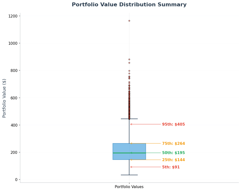
Key Percentiles Explained:

5th percentile: Only 5% of scenarios do worse than this (downside risk)
25th percentile: First quartile - represents poor but not catastrophic outcomes
50th percentile (median): Half of scenarios do better, half do worse
75th percentile: Third quartile - represents good outcomes
95th percentile: Only 5% of scenarios do better than this (upside potential)

These risk metrics are calculated below:

Understanding Median vs Expected ReturnLink Copied

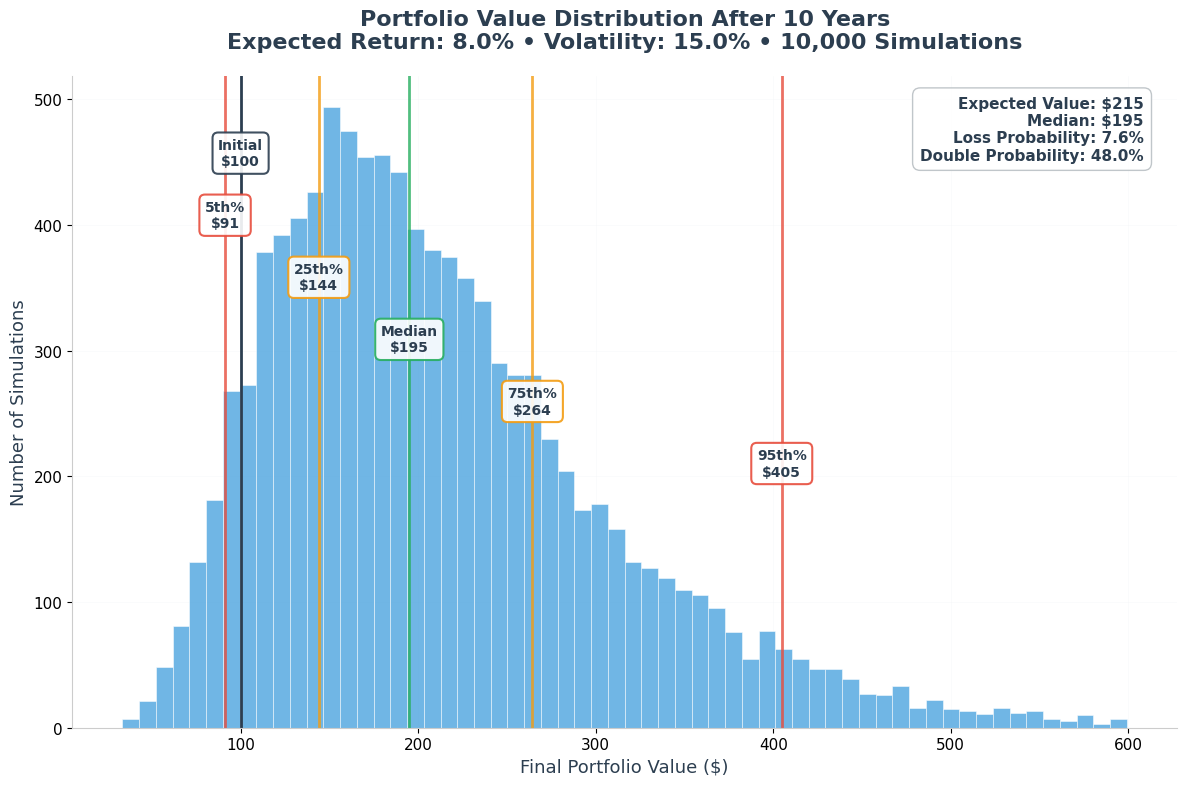
Key Insight: Notice that the median ($195) is lower than the expected value ($215). This is not an error - it's a fundamental characteristic of investment returns.

Why This Happens:

Skewed Distribution: Investment returns exhibit positive skewness - there are occasional very large gains that pull the average upward, but losses are bounded (you can't lose more than 100%).
Arithmetic vs Geometric: The expected value uses arithmetic averaging of outcomes, while actual compound growth follows geometric progression. A few extremely successful scenarios significantly raise the arithmetic mean.
Practical Implication: The median represents the "typical" outcome - half of all scenarios do better, half do worse. The expected value is mathematically correct but influenced by extreme positive outcomes.

Real-World Meaning: If you ran this investment 100 times, you'd be more likely to end up near the median ($195) than the expected value ($215). The expected value includes the impact of those rare scenarios where your portfolio might grow to $500+ or even $1000+.

6. Creating Meaningful VisualizationsLink Copied

We'll create a series of focused visualizations to understand different aspects of our Monte Carlo simulation results. Each chart reveals different insights about the investment risk and return profile.

6.1 Portfolio Value DistributionLink Copied

The histogram shows the spread of possible outcomes from our Monte Carlo simulation. This visualization helps us understand the likelihood of different portfolio values after 10 years.

In[6]:

# Portfolio Value Distribution Histogram
fig, ax = plt.subplots(figsize=(12, 8))

# Filter out values over $600 to focus on the main distribution
filtered_values = final_portfolio_values[final_portfolio_values <= 600]

# Creating histogram with modern aesthetics
n, bins, patches = ax.hist(filtered_values, bins=60, alpha=0.7, 
                          edgecolor='white', linewidth=0.5, color='#3498db')

# Adding vertical lines for key percentiles with better positioning
percentiles = [5, 25, 50, 75, 95]
percentile_values = np.percentile(final_portfolio_values, percentiles)
colors = ['#e74c3c', '#f39c12', '#27ae60', '#f39c12', '#e74c3c']
labels = ['5th%', '25th%', 'Median', '75th%', '95th%']

max_height = n.max()
for i, (perc, val, color, label) in enumerate(zip(percentiles, percentile_values, colors, labels)):
    if val <= 600:
        ax.axvline(val, color=color, linestyle='-', linewidth=2, alpha=0.8)
        ax.text(val, max_height * (0.85 - i * 0.1), f'{label}\n${val:.0f}', 
                ha='center', va='top', fontweight='600', fontsize=10,
                bbox=dict(boxstyle="round,pad=0.4", facecolor='white', alpha=0.9, edgecolor=color, linewidth=1.5),
                color='#2c3e50')

# Adding initial investment line for reference
ax.axvline(INITIAL_INVESTMENT, color='#2c3e50', linestyle='-', linewidth=2)
ax.text(INITIAL_INVESTMENT, max_height * 0.95, f'Initial\n${INITIAL_INVESTMENT:.0f}', 
        ha='center', va='top', fontweight='600', fontsize=10,
        bbox=dict(boxstyle="round,pad=0.4", facecolor='white', alpha=0.9, edgecolor='#2c3e50', linewidth=1.5),
        color='#2c3e50')

# Calculate excluded scenarios
excluded_count = len(final_portfolio_values) - len(filtered_values)
excluded_pct = (excluded_count / len(final_portfolio_values)) * 100

ax.set_title(f"Portfolio Value Distribution After {YEARS} Years\n"
             f"Expected Return: {MU:.1%} • Volatility: {SIGMA:.1%} • {N_ITER:,} Simulations",
             fontsize=16, fontweight='600', pad=20, color='#2c3e50')
ax.set_xlabel("Final Portfolio Value ($)", fontsize=13, fontweight='500', color='#2c3e50')
ax.set_ylabel("Number of Simulations", fontsize=13, fontweight='500', color='#2c3e50')

# Adding summary statistics in a cleaner box
stats_text = f"Expected Value: ${final_portfolio_values.mean():.0f}\n" \
            f"Median: ${np.median(final_portfolio_values):.0f}\n" \
            f"Loss Probability: {prob_loss:.1f}%\n" \
            f"Double Probability: {prob_double:.1f}%"

ax.text(0.97, 0.97, stats_text, transform=ax.transAxes, fontsize=11, fontweight='600',
        va='top', ha='right', color='#2c3e50',
        bbox=dict(boxstyle="round,pad=0.5", facecolor='white', alpha=0.95, 
                  edgecolor='#bdc3c7', linewidth=1))

# Clean up the plot
ax.grid(True, alpha=0.3, color='#ecf0f1')
ax.set_axisbelow(True)

plt.tight_layout()
plt.show()

# Portfolio Value Distribution Histogram
fig, ax = plt.subplots(figsize=(12, 8))

# Filter out values over $600 to focus on the main distribution
filtered_values = final_portfolio_values[final_portfolio_values <= 600]

# Creating histogram with modern aesthetics
n, bins, patches = ax.hist(filtered_values, bins=60, alpha=0.7, 
                          edgecolor='white', linewidth=0.5, color='#3498db')

# Adding vertical lines for key percentiles with better positioning
percentiles = [5, 25, 50, 75, 95]
percentile_values = np.percentile(final_portfolio_values, percentiles)
colors = ['#e74c3c', '#f39c12', '#27ae60', '#f39c12', '#e74c3c']
labels = ['5th%', '25th%', 'Median', '75th%', '95th%']

max_height = n.max()
for i, (perc, val, color, label) in enumerate(zip(percentiles, percentile_values, colors, labels)):
    if val <= 600:
        ax.axvline(val, color=color, linestyle='-', linewidth=2, alpha=0.8)
        ax.text(val, max_height * (0.85 - i * 0.1), f'{label}\n${val:.0f}', 
                ha='center', va='top', fontweight='600', fontsize=10,
                bbox=dict(boxstyle="round,pad=0.4", facecolor='white', alpha=0.9, edgecolor=color, linewidth=1.5),
                color='#2c3e50')

# Adding initial investment line for reference
ax.axvline(INITIAL_INVESTMENT, color='#2c3e50', linestyle='-', linewidth=2)
ax.text(INITIAL_INVESTMENT, max_height * 0.95, f'Initial\n${INITIAL_INVESTMENT:.0f}', 
        ha='center', va='top', fontweight='600', fontsize=10,
        bbox=dict(boxstyle="round,pad=0.4", facecolor='white', alpha=0.9, edgecolor='#2c3e50', linewidth=1.5),
        color='#2c3e50')

# Calculate excluded scenarios
excluded_count = len(final_portfolio_values) - len(filtered_values)
excluded_pct = (excluded_count / len(final_portfolio_values)) * 100

ax.set_title(f"Portfolio Value Distribution After {YEARS} Years\n"
             f"Expected Return: {MU:.1%} • Volatility: {SIGMA:.1%} • {N_ITER:,} Simulations",
             fontsize=16, fontweight='600', pad=20, color='#2c3e50')
ax.set_xlabel("Final Portfolio Value ($)", fontsize=13, fontweight='500', color='#2c3e50')
ax.set_ylabel("Number of Simulations", fontsize=13, fontweight='500', color='#2c3e50')

# Adding summary statistics in a cleaner box
stats_text = f"Expected Value: ${final_portfolio_values.mean():.0f}\n" \
            f"Median: ${np.median(final_portfolio_values):.0f}\n" \
            f"Loss Probability: {prob_loss:.1f}%\n" \
            f"Double Probability: {prob_double:.1f}%"

ax.text(0.97, 0.97, stats_text, transform=ax.transAxes, fontsize=11, fontweight='600',
        va='top', ha='right', color='#2c3e50',
        bbox=dict(boxstyle="round,pad=0.5", facecolor='white', alpha=0.95, 
                  edgecolor='#bdc3c7', linewidth=1))

# Clean up the plot
ax.grid(True, alpha=0.3, color='#ecf0f1')
ax.set_axisbelow(True)

plt.tight_layout()
plt.show()

Out[6]:

Visualization

6.2 Box Plot SummaryLink Copied

The box plot provides a concise statistical summary, highlighting the quartiles, median, and outliers in our portfolio value distribution.

In[7]:

# Box Plot showing percentile ranges with modern styling
fig, ax = plt.subplots(figsize=(10, 8))

box_data = [final_portfolio_values]
bp = ax.boxplot(box_data, patch_artist=True, tick_labels=['Portfolio Values'],
               medianprops=dict(color='#27ae60', linewidth=2.5),
               boxprops=dict(facecolor='#3498db', alpha=0.6, edgecolor='#2980b9', linewidth=1.5),
               whiskerprops=dict(color='#34495e', linewidth=1.5),
               capprops=dict(color='#34495e', linewidth=1.5),
               flierprops=dict(marker='o', markerfacecolor='#e74c3c', alpha=0.5, markersize=4))

# Adding percentile annotations with cleaner styling
percentiles_to_show = [5, 25, 50, 75, 95]
perc_values = np.percentile(final_portfolio_values, percentiles_to_show)
colors = ['#e74c3c', '#f39c12', '#27ae60', '#f39c12', '#e74c3c']

for i, (perc, val, color) in enumerate(zip(percentiles_to_show, perc_values, colors)):
    ax.annotate(f'{perc}th: ${val:.0f}', 
                xy=(1, val), xytext=(1.15, val),
                fontsize=11, ha='left', va='center', fontweight='600',
                color=color,
                arrowprops=dict(arrowstyle='->', color=color, alpha=0.7, lw=1.2))

ax.set_title('Portfolio Value Distribution Summary', 
             fontweight='600', fontsize=16, color='#2c3e50', pad=20)
ax.set_ylabel('Portfolio Value ($)', fontweight='500', fontsize=13, color='#2c3e50')
ax.grid(True, alpha=0.3, color='#ecf0f1', axis='y')
ax.set_axisbelow(True)

# Remove top and right spines for cleaner look
ax.spines['top'].set_visible(False)
ax.spines['right'].set_visible(False)
ax.spines['left'].set_color('#bdc3c7')
ax.spines['bottom'].set_color('#bdc3c7')

plt.tight_layout()
plt.show()

# Box Plot showing percentile ranges with modern styling
fig, ax = plt.subplots(figsize=(10, 8))

box_data = [final_portfolio_values]
bp = ax.boxplot(box_data, patch_artist=True, tick_labels=['Portfolio Values'],
               medianprops=dict(color='#27ae60', linewidth=2.5),
               boxprops=dict(facecolor='#3498db', alpha=0.6, edgecolor='#2980b9', linewidth=1.5),
               whiskerprops=dict(color='#34495e', linewidth=1.5),
               capprops=dict(color='#34495e', linewidth=1.5),
               flierprops=dict(marker='o', markerfacecolor='#e74c3c', alpha=0.5, markersize=4))

# Adding percentile annotations with cleaner styling
percentiles_to_show = [5, 25, 50, 75, 95]
perc_values = np.percentile(final_portfolio_values, percentiles_to_show)
colors = ['#e74c3c', '#f39c12', '#27ae60', '#f39c12', '#e74c3c']

for i, (perc, val, color) in enumerate(zip(percentiles_to_show, perc_values, colors)):
    ax.annotate(f'{perc}th: ${val:.0f}', 
                xy=(1, val), xytext=(1.15, val),
                fontsize=11, ha='left', va='center', fontweight='600',
                color=color,
                arrowprops=dict(arrowstyle='->', color=color, alpha=0.7, lw=1.2))

ax.set_title('Portfolio Value Distribution Summary', 
             fontweight='600', fontsize=16, color='#2c3e50', pad=20)
ax.set_ylabel('Portfolio Value ($)', fontweight='500', fontsize=13, color='#2c3e50')
ax.grid(True, alpha=0.3, color='#ecf0f1', axis='y')
ax.set_axisbelow(True)

# Remove top and right spines for cleaner look
ax.spines['top'].set_visible(False)
ax.spines['right'].set_visible(False)
ax.spines['left'].set_color('#bdc3c7')
ax.spines['bottom'].set_color('#bdc3c7')

plt.tight_layout()
plt.show()

Out[7]:

Visualization

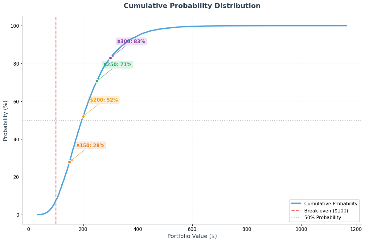
6.3 Cumulative Distribution Function (CDF)Link Copied

The CDF shows the probability of achieving different portfolio values. This helps answer questions like "What's the probability my portfolio will be worth at least $200?"

In[8]:

# Cumulative Distribution Function (CDF) with modern styling
fig, ax = plt.subplots(figsize=(12, 8))

sorted_values = np.sort(final_portfolio_values)
cumulative_prob = np.arange(1, len(sorted_values) + 1) / len(sorted_values)

# Main CDF line with gradient-like effect
ax.plot(sorted_values, cumulative_prob * 100, linewidth=3, color='#3498db', 
        label='Cumulative Probability', alpha=0.9)

# Reference lines
ax.axvline(INITIAL_INVESTMENT, color='#e74c3c', linestyle='--', alpha=0.8, 
          linewidth=2, label='Break-even ($100)')
ax.axhline(50, color='#95a5a6', linestyle=':', alpha=0.7, 
          linewidth=2, label='50% Probability')

# Key probability markers with modern styling
key_values = [150, 200, 250, 300]
marker_colors = ['#e67e22', '#f39c12', '#27ae60', '#8e44ad']

for val, color in zip(key_values, marker_colors):
    prob = (final_portfolio_values <= val).mean() * 100
    ax.plot(val, prob, 'o', markersize=8, color=color, 
           markeredgecolor='white', markeredgewidth=2, zorder=5)
    ax.annotate(f'${val}: {prob:.0f}%', 
               xy=(val, prob), xytext=(val+25, prob+8),
               fontsize=11, ha='left', fontweight='600', color=color,
               bbox=dict(boxstyle="round,pad=0.3", facecolor=color, alpha=0.15, 
                        edgecolor=color, linewidth=1),
               arrowprops=dict(arrowstyle='->', color=color, alpha=0.7, lw=1.2))

ax.set_title('Cumulative Probability Distribution', 
             fontweight='600', fontsize=16, color='#2c3e50', pad=20)
ax.set_xlabel('Portfolio Value ($)', fontweight='500', fontsize=13, color='#2c3e50')
ax.set_ylabel('Probability (%)', fontweight='500', fontsize=13, color='#2c3e50')

# Modern legend styling
ax.legend(fontsize=11, frameon=True, fancybox=True, shadow=False,
         facecolor='white', edgecolor='#bdc3c7', framealpha=0.9)

# Clean grid and spines
ax.grid(True, alpha=0.3, color='#ecf0f1')
ax.set_axisbelow(True)
ax.spines['top'].set_visible(False)
ax.spines['right'].set_visible(False)
ax.spines['left'].set_color('#bdc3c7')
ax.spines['bottom'].set_color('#bdc3c7')

plt.tight_layout()
plt.show()

# Cumulative Distribution Function (CDF) with modern styling
fig, ax = plt.subplots(figsize=(12, 8))

sorted_values = np.sort(final_portfolio_values)
cumulative_prob = np.arange(1, len(sorted_values) + 1) / len(sorted_values)

# Main CDF line with gradient-like effect
ax.plot(sorted_values, cumulative_prob * 100, linewidth=3, color='#3498db', 
        label='Cumulative Probability', alpha=0.9)

# Reference lines
ax.axvline(INITIAL_INVESTMENT, color='#e74c3c', linestyle='--', alpha=0.8, 
          linewidth=2, label='Break-even ($100)')
ax.axhline(50, color='#95a5a6', linestyle=':', alpha=0.7, 
          linewidth=2, label='50% Probability')

# Key probability markers with modern styling
key_values = [150, 200, 250, 300]
marker_colors = ['#e67e22', '#f39c12', '#27ae60', '#8e44ad']

for val, color in zip(key_values, marker_colors):
    prob = (final_portfolio_values <= val).mean() * 100
    ax.plot(val, prob, 'o', markersize=8, color=color, 
           markeredgecolor='white', markeredgewidth=2, zorder=5)
    ax.annotate(f'${val}: {prob:.0f}%', 
               xy=(val, prob), xytext=(val+25, prob+8),
               fontsize=11, ha='left', fontweight='600', color=color,
               bbox=dict(boxstyle="round,pad=0.3", facecolor=color, alpha=0.15, 
                        edgecolor=color, linewidth=1),
               arrowprops=dict(arrowstyle='->', color=color, alpha=0.7, lw=1.2))

ax.set_title('Cumulative Probability Distribution', 
             fontweight='600', fontsize=16, color='#2c3e50', pad=20)
ax.set_xlabel('Portfolio Value ($)', fontweight='500', fontsize=13, color='#2c3e50')
ax.set_ylabel('Probability (%)', fontweight='500', fontsize=13, color='#2c3e50')

# Modern legend styling
ax.legend(fontsize=11, frameon=True, fancybox=True, shadow=False,
         facecolor='white', edgecolor='#bdc3c7', framealpha=0.9)

# Clean grid and spines
ax.grid(True, alpha=0.3, color='#ecf0f1')
ax.set_axisbelow(True)
ax.spines['top'].set_visible(False)
ax.spines['right'].set_visible(False)
ax.spines['left'].set_color('#bdc3c7')
ax.spines['bottom'].set_color('#bdc3c7')

plt.tight_layout()
plt.show()

Out[8]:

Visualization

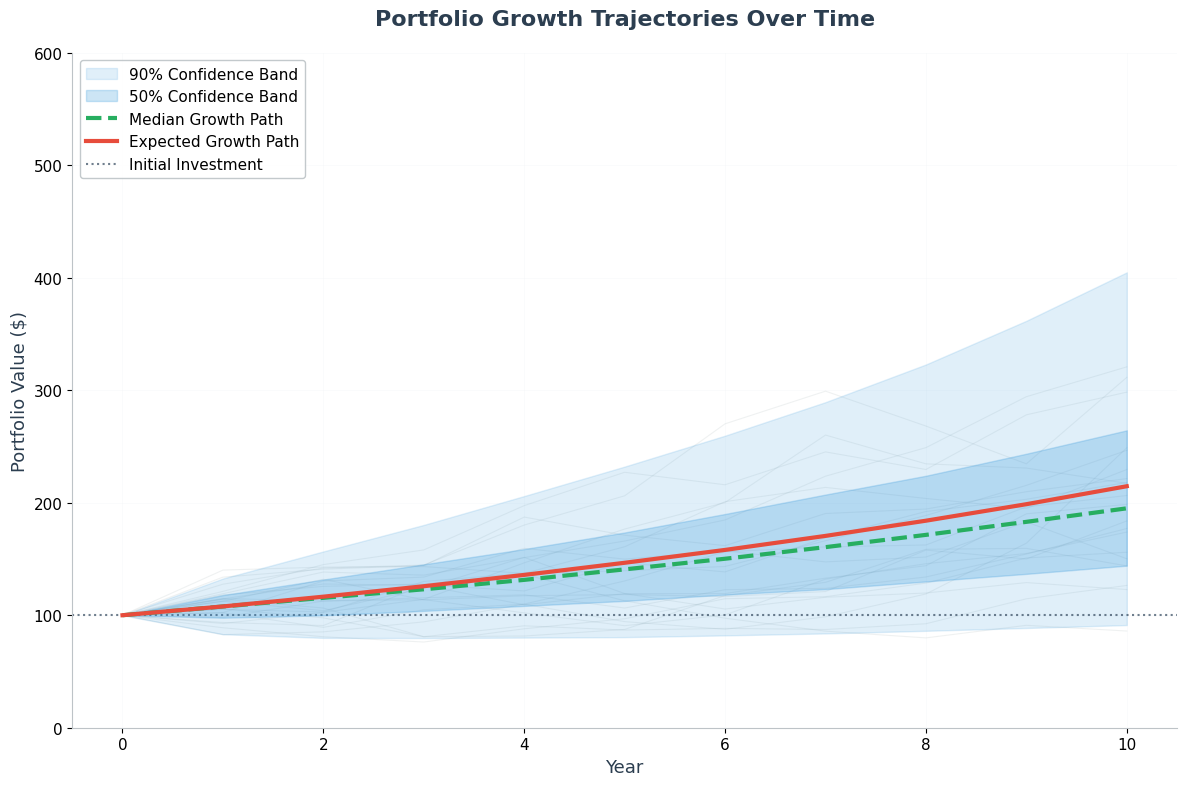
6.4 Portfolio Growth Over TimeLink Copied

This visualization shows how portfolio values evolve year by year, demonstrating the compound growth effect and the confidence band around the expected path.

In[9]:

# Portfolio growth over time with modern styling
fig, ax = plt.subplots(figsize=(12, 8))

# Calculate portfolio values for each year for sample scenarios
sample_scenarios = annual_returns[:100, :]  # First 100 scenarios
portfolio_evolution = np.zeros((100, YEARS + 1))  # +1 for initial value
portfolio_evolution[:, 0] = INITIAL_INVESTMENT

for year in range(YEARS):
    portfolio_evolution[:, year + 1] = portfolio_evolution[:, year] * (1 + sample_scenarios[:, year])

# Plot sample paths (very light gray lines)
for i in range(20):
    ax.plot(np.arange(YEARS + 1), portfolio_evolution[i, :], 
           alpha=0.15, color='#95a5a6', linewidth=0.8, zorder=1)

# Calculate evolution for all scenarios for confidence bands
all_portfolio_evolution = np.zeros((N_ITER, YEARS + 1))
all_portfolio_evolution[:, 0] = INITIAL_INVESTMENT

for year in range(YEARS):
    all_portfolio_evolution[:, year + 1] = all_portfolio_evolution[:, year] * (1 + annual_returns[:, year])

# Add confidence bands with gradient-like colors
percentile_5 = np.percentile(all_portfolio_evolution, 5, axis=0)
percentile_95 = np.percentile(all_portfolio_evolution, 95, axis=0)
percentile_25 = np.percentile(all_portfolio_evolution, 25, axis=0)
percentile_75 = np.percentile(all_portfolio_evolution, 75, axis=0)

# Fill confidence bands with different opacities
ax.fill_between(np.arange(YEARS + 1), percentile_5, percentile_95, 
               alpha=0.15, color='#3498db', label='90% Confidence Band', zorder=2)
ax.fill_between(np.arange(YEARS + 1), percentile_25, percentile_75, 
               alpha=0.25, color='#3498db', label='50% Confidence Band', zorder=3)

# Plot median line
median_evolution = np.percentile(all_portfolio_evolution, 50, axis=0)
ax.plot(np.arange(YEARS + 1), median_evolution, linewidth=3, color='#27ae60', 
        linestyle='--', label='Median Growth Path', zorder=4)

# Plot average evolution
mean_evolution = all_portfolio_evolution.mean(axis=0)
ax.plot(np.arange(YEARS + 1), mean_evolution, linewidth=3, color='#e74c3c', 
        label='Expected Growth Path', zorder=5)

# Add initial investment reference line
ax.axhline(INITIAL_INVESTMENT, color='#34495e', linestyle=':', alpha=0.7, 
          linewidth=1.5, label='Initial Investment')

ax.set_title('Portfolio Growth Trajectories Over Time', 
             fontweight='600', fontsize=16, color='#2c3e50', pad=20)
ax.set_xlabel('Year', fontweight='500', fontsize=13, color='#2c3e50')
ax.set_ylabel('Portfolio Value ($)', fontweight='500', fontsize=13, color='#2c3e50')

# Modern legend styling
ax.legend(fontsize=11, frameon=True, fancybox=True, shadow=False,
         facecolor='white', edgecolor='#bdc3c7', framealpha=0.9,
         loc='upper left')

# Clean grid and spines
ax.grid(True, alpha=0.3, color='#ecf0f1')
ax.set_axisbelow(True)
ax.spines['top'].set_visible(False)
ax.spines['right'].set_visible(False)
ax.spines['left'].set_color('#bdc3c7')
ax.spines['bottom'].set_color('#bdc3c7')

# Set reasonable y-axis limits to avoid extreme outliers
ax.set_ylim(0, 600)

plt.tight_layout()
plt.show()

# Portfolio growth over time with modern styling
fig, ax = plt.subplots(figsize=(12, 8))

# Calculate portfolio values for each year for sample scenarios
sample_scenarios = annual_returns[:100, :]  # First 100 scenarios
portfolio_evolution = np.zeros((100, YEARS + 1))  # +1 for initial value
portfolio_evolution[:, 0] = INITIAL_INVESTMENT

for year in range(YEARS):
    portfolio_evolution[:, year + 1] = portfolio_evolution[:, year] * (1 + sample_scenarios[:, year])

# Plot sample paths (very light gray lines)
for i in range(20):
    ax.plot(np.arange(YEARS + 1), portfolio_evolution[i, :], 
           alpha=0.15, color='#95a5a6', linewidth=0.8, zorder=1)

# Calculate evolution for all scenarios for confidence bands
all_portfolio_evolution = np.zeros((N_ITER, YEARS + 1))
all_portfolio_evolution[:, 0] = INITIAL_INVESTMENT

for year in range(YEARS):
    all_portfolio_evolution[:, year + 1] = all_portfolio_evolution[:, year] * (1 + annual_returns[:, year])

# Add confidence bands with gradient-like colors
percentile_5 = np.percentile(all_portfolio_evolution, 5, axis=0)
percentile_95 = np.percentile(all_portfolio_evolution, 95, axis=0)
percentile_25 = np.percentile(all_portfolio_evolution, 25, axis=0)
percentile_75 = np.percentile(all_portfolio_evolution, 75, axis=0)

# Fill confidence bands with different opacities
ax.fill_between(np.arange(YEARS + 1), percentile_5, percentile_95, 
               alpha=0.15, color='#3498db', label='90% Confidence Band', zorder=2)
ax.fill_between(np.arange(YEARS + 1), percentile_25, percentile_75, 
               alpha=0.25, color='#3498db', label='50% Confidence Band', zorder=3)

# Plot median line
median_evolution = np.percentile(all_portfolio_evolution, 50, axis=0)
ax.plot(np.arange(YEARS + 1), median_evolution, linewidth=3, color='#27ae60', 
        linestyle='--', label='Median Growth Path', zorder=4)

# Plot average evolution
mean_evolution = all_portfolio_evolution.mean(axis=0)
ax.plot(np.arange(YEARS + 1), mean_evolution, linewidth=3, color='#e74c3c', 
        label='Expected Growth Path', zorder=5)

# Add initial investment reference line
ax.axhline(INITIAL_INVESTMENT, color='#34495e', linestyle=':', alpha=0.7, 
          linewidth=1.5, label='Initial Investment')

ax.set_title('Portfolio Growth Trajectories Over Time', 
             fontweight='600', fontsize=16, color='#2c3e50', pad=20)
ax.set_xlabel('Year', fontweight='500', fontsize=13, color='#2c3e50')
ax.set_ylabel('Portfolio Value ($)', fontweight='500', fontsize=13, color='#2c3e50')

# Modern legend styling
ax.legend(fontsize=11, frameon=True, fancybox=True, shadow=False,
         facecolor='white', edgecolor='#bdc3c7', framealpha=0.9,
         loc='upper left')

# Clean grid and spines
ax.grid(True, alpha=0.3, color='#ecf0f1')
ax.set_axisbelow(True)
ax.spines['top'].set_visible(False)
ax.spines['right'].set_visible(False)
ax.spines['left'].set_color('#bdc3c7')
ax.spines['bottom'].set_color('#bdc3c7')

# Set reasonable y-axis limits to avoid extreme outliers
ax.set_ylim(0, 600)

plt.tight_layout()
plt.show()

Out[9]:

Visualization

7. Conclusion: The Power of Monte Carlo SimulationLink Copied

Monte Carlo simulation transforms investment uncertainty from guesswork into quantified risk assessment. By running 10,000 possible scenarios, we've mapped the full landscape of potential outcomes for our investment.

Key Monte Carlo Insights:

Probabilistic Thinking: Rather than a single "expected" return, we now understand the full distribution of possibilities
Risk Quantification: We can precisely state there's a 7.6% chance of losing money and a 48% chance of doubling our investment
Confidence Intervals: We're 90% confident our final portfolio will be between $91 and$ 405

Why Monte Carlo Works:

Captures Uncertainty: Markets are inherently random - Monte Carlo embraces this reality rather than ignoring it
Compound Effects: Shows how volatility compounds over time, revealing both upside potential and downside risk
Decision Support: Provides the statistical foundation for rational investment decisions

The Monte Carlo Advantage:

Traditional financial planning might say "expect 8% returns." Monte Carlo simulation reveals that while 8% is the average, actual outcomes range dramatically. This knowledge is power - it enables better risk management, more realistic expectations, and informed decision-making.

Monte Carlo simulation is not just a mathematical exercise; it's a lens for understanding uncertainty in any complex system where randomness plays a crucial role.

Comments

Reference

BIBTEXAcademic

@misc{simulatingstockmarketreturnsusingmontecarlo, author = {Michael Brenndoerfer}, title = {Simulating stock market returns using Monte Carlo}, year = {2025}, url = {https://mbrenndoerfer.com/writing/introduction-stock-market-monte-carlo-simulation}, organization = {mbrenndoerfer.com}, note = {Accessed: 2025-12-09} }

APAAcademic

Michael Brenndoerfer (2025). Simulating stock market returns using Monte Carlo. Retrieved from https://mbrenndoerfer.com/writing/introduction-stock-market-monte-carlo-simulation

MLAAcademic

Michael Brenndoerfer. "Simulating stock market returns using Monte Carlo." 2025. Web. 12/9/2025. <https://mbrenndoerfer.com/writing/introduction-stock-market-monte-carlo-simulation>.

CHICAGOAcademic

Michael Brenndoerfer. "Simulating stock market returns using Monte Carlo." Accessed 12/9/2025. https://mbrenndoerfer.com/writing/introduction-stock-market-monte-carlo-simulation.

HARVARDAcademic

Michael Brenndoerfer (2025) 'Simulating stock market returns using Monte Carlo'. Available at: https://mbrenndoerfer.com/writing/introduction-stock-market-monte-carlo-simulation (Accessed: 12/9/2025).

SimpleBasic

Michael Brenndoerfer (2025). Simulating stock market returns using Monte Carlo. https://mbrenndoerfer.com/writing/introduction-stock-market-monte-carlo-simulation

Direct link:

https://mbrenndoerfer.com/writing/introduction-stock-market-monte-carlo-simulation

About the author: Michael Brenndoerfer

All opinions expressed here are my own and do not reflect the views of my employer.

Michael currently works as an Associate Director of Data Science at EQT Partners in Singapore, where he drives AI and data initiatives across private capital investments.

With over a decade of experience spanning private equity, management consulting, and software engineering, he specializes in building and scaling analytics capabilities from the ground up. He has published research in leading AI conferences and holds expertise in machine learning, natural language processing, and value creation through data.

View Full Resume Publications Contact Books

InteractiveSimulating stock market returns using Monte Carlo

A Simple Yet Complete Tutorial on Estimating Long-Term Investment ReturnsLink Copied

Learning ObjectivesLink Copied

What We'll BuildLink Copied

Key Concepts CoveredLink Copied

1. Setting Up The EnvironmentLink Copied

2. Defining The Simulation ParametersLink Copied

Understanding the Financial ModelLink Copied

Why These Numbers?Link Copied

3. Generating Random ReturnsLink Copied

The Heart of Monte Carlo SimulationLink Copied

Understanding the Output StructureLink Copied

4. Computing Final Portfolio ValuesLink Copied

The Compound Growth FormulaLink Copied

Why This WorksLink Copied

Example CalculationLink Copied

5. Statistical Analysis and Risk AssessmentLink Copied

Understanding Percentiles and Risk MetricsLink Copied

Understanding Median vs Expected ReturnLink Copied

6. Creating Meaningful VisualizationsLink Copied

6.1 Portfolio Value DistributionLink Copied

6.2 Box Plot SummaryLink Copied

6.3 Cumulative Distribution Function (CDF)Link Copied

6.4 Portfolio Growth Over TimeLink Copied

7. Conclusion: The Power of Monte Carlo SimulationLink Copied

Comments

Reference

About the author: Michael Brenndoerfer

Related Content

Skip-gram Model: Learning Word Embeddings by Predicting Context

Singular Value Decomposition: Matrix Factorization for Word Embeddings & LSA

Pointwise Mutual Information: Measuring Word Associations in NLP

Stay updated