Word Embeddings: From Word2Vec to GloVe - Understanding Distributed Representations

How do we represent words as numbers? This question has driven NLP research for decades. Early approaches used one-hot encoding: each word gets a unique vector where all values are zero except one position. "cat" might be [1, 0, 0, 0, ...], "dog" might be [0, 1, 0, 0, ...]. This works, but it's fundamentally limited. These vectors tell us nothing about relationships between words. "cat" and "dog" are as similar as "cat" and "airplane" in one-hot space.

Word embeddings solve this by learning dense, low-dimensional vectors where semantically similar words have similar vector representations. Instead of sparse one-hot vectors with thousands of dimensions, we get compact vectors (typically 100-300 dimensions) where words with related meanings cluster together in vector space. The distance between "cat" and "dog" becomes small, while "cat" and "airplane" remain far apart.

The breakthrough came from a simple insight: words that appear in similar contexts tend to have similar meanings. This distributional hypothesis, dating back to linguist J.R. Firth's 1957 observation that "you shall know a word by the company it keeps," became the foundation for modern word embedding methods. Word2Vec and GloVe, the two most influential embedding algorithms, both exploit this principle, but through different mathematical approaches.

Word embeddings transformed NLP by enabling models to capture semantic relationships directly from data. They unlocked transfer learning: embeddings trained on massive text corpora could be reused across tasks, dramatically improving performance on downstream applications with limited training data. Today, word embeddings are foundational to everything from search engines to chatbots, though they've been largely superseded by contextual embeddings from transformers.

Before word embeddings, NLP systems relied on sparse, high-dimensional representations that couldn't capture semantic relationships. Understanding these limitations helps explain why embeddings represented a significant advance in NLP.

One-hot encoding represents each word as a binary vector where exactly one position is 1 and all others are 0. If your vocabulary has 10,000 words, each word gets a 10,000-dimensional vector:

Notice that "cat" and "dog" are as different as "cat" and "airplane" in this representation. The dot product between any two different one-hot vectors is always zero, meaning we can't measure similarity. This is a fundamental limitation: one-hot encoding treats all words as equally different.

One-hot encoding also suffers from the curse of dimensionality. With a vocabulary of 50,000 words (typical for English), each word requires a 50,000-dimensional vector. Most of these dimensions are wasted: 99.998% of the vector is zeros. This creates several problems:

• Storage inefficiency: Storing millions of sparse vectors wastes memory
• Computational overhead: Operations on sparse vectors are slower
• No generalization: A model can't learn that "running" and "runs" are related if they're represented as completely orthogonal vectors

What we need is a dense representation where:

1. Similarity is measurable: Words with related meanings have similar vectors
2. Dimensionality is manageable: Compact vectors (100-300 dimensions) instead of thousands
3. Relationships are preserved: Analogies like "king - man + woman = queen" emerge naturally

Word embeddings provide exactly this. They learn dense vectors where semantic relationships are encoded in the geometry of the vector space.

Word2Vec, introduced by Mikolov et al. in 2013, learns word embeddings by predicting words from their local context. The key insight is simple: train a neural network to predict surrounding words, and the learned weights become meaningful word representations.

Word2Vec offers two architectures: Continuous Bag of Words (CBOW) and Skip-gram. Both use shallow neural networks, but they solve inverse problems:

• CBOW: Predicts the center word from surrounding context words
• Skip-gram: Predicts surrounding context words from the center word

Skip-gram typically performs better on rare words and is more commonly used, so we'll focus on it. The principles apply to both.

Let's start with a simple observation. When you read the sentence "The quick brown fox jumps over the lazy dog," you immediately understand that "fox" is related to "quick," "brown," "jumps," and "over" because they appear together. This is the distributional hypothesis in action: words that appear in similar contexts tend to have similar meanings.

Word2Vec formalizes this intuition through a prediction task. Instead of asking "what do these words mean?", we ask "can we predict which words appear together?" The key insight is that learning to predict context automatically discovers semantic relationships. Words that appear in similar contexts will need similar internal representations to make accurate predictions, and these representations become our embeddings.

Skip-gram takes a center word and tries to predict words that appear nearby in the text. Consider our example sentence: "The quick brown fox jumps over the lazy dog." If "fox" is our center word and we use a window size of 2, we want to predict: "quick", "brown", "jumps", "over".

The architecture is surprisingly simple, consisting of just three layers:

1. Input layer: One-hot encoded center word (vocabulary size $V$). This is a sparse vector where exactly one position is 1, indicating which word we're currently considering.

2. Hidden layer: A linear projection to embedding dimension $d$ (typically 100-300). When we multiply the one-hot vector by the weight matrix, we're selecting one row from that matrix, which is the embedding vector for our center word.

3. Output layer: A softmax over the entire vocabulary to predict which word appears in the context. This gives us a probability distribution over all possible context words.

The key insight is that the weight matrix connecting input to hidden layer becomes our word embeddings. Each row of this matrix is the embedding vector for one word. As the network learns to predict context words accurately, it must learn to place similar words (those with similar contexts) in similar regions of embedding space.

Now let's formalize this intuition into a mathematical objective. We want to maximize the probability of observing the actual context words given our center word. For a center word $w_t$ at position $t$ and a context window of size $c$, we observe context words $w_{t-c}, \ldots, w_{t-1}, w_{t+1}, \ldots, w_{t+c}$.

Our goal is to maximize:

This probability tells us: "Given that we see word $w_t$ as the center word, how likely are we to see these specific context words around it?" To make this tractable, we make a simplifying assumption: context words are independent given the center word. This means the probability of seeing "quick" and "brown" around "fox" is the product of seeing each individually:

where:

• $w_t$: the center word at position $t$ in the corpus
• $w_{t+j}$: a context word at position $t+j$ (within the window around $w_t$)
• $c$: the context window size (typically 5-10 words on each side)
• $P(w_{t+j} | w_t)$: the conditional probability of observing context word $w_{t+j}$ given center word $w_t$

This assumption isn't perfectly true (words in context aren't truly independent), but it works well in practice and makes the math manageable. Each term $P(w_{t+j} | w_t)$ asks: "Given center word $w_t$, what's the probability that word $w_{t+j}$ appears in the context?"

To convert this into a loss function we can minimize (standard practice in machine learning), we take the negative logarithm:

where:

• $L$: the loss function to minimize
• The negative sign converts maximization (of probabilities) to minimization (standard in optimization)
• The logarithm converts the product into a sum, which is numerically more stable and has better gradient properties

Why the negative logarithm? Two reasons: (1) maximizing probabilities is equivalent to minimizing negative log probabilities, and (2) logarithms convert products into sums, which are easier to work with numerically and have better gradient properties.

Now we need to compute $P(w_{t+j} | w_t)$, the probability that a specific context word appears given the center word. This is where embeddings enter the picture.

We compute this probability using the softmax function over the entire vocabulary:

where:

• $w_I$: the input (center) word
• $w_O$: the output (context) word
• $\mathbf{v}_{w_I} \in \mathbb{R}^d$: the input embedding vector for word $w_I$ (center word representation), where $d$ is the embedding dimension
• $\mathbf{v}_{w_O} \in \mathbb{R}^d$: the output embedding vector for word $w_O$ (context word representation)
• $\mathbf{v}_{w_O}^T \mathbf{v}_{w_I}$: the dot product (scalar) measuring similarity between the two embedding vectors
• $V$: the vocabulary size (total number of unique words)
• $\exp(\cdot)$: the exponential function, which amplifies differences in dot products
• The numerator $\exp(\mathbf{v}_{w_O}^T \mathbf{v}_{w_I})$ measures the "compatibility" between center and context words
• The denominator $\sum_{w=1}^{V} \exp(\mathbf{v}_w^T \mathbf{v}_{w_I})$ normalizes over all possible context words, ensuring probabilities sum to 1

This is the softmax function, which converts raw similarity scores (dot products) into a probability distribution over the vocabulary.

Why the dot product? The dot product $\mathbf{v}_{w_O}^T \mathbf{v}_{w_I}$ measures how similar two vectors are. If embeddings are similar (point in similar directions), the dot product is large. If they're different (point in different directions), the dot product is small. The exponential function amplifies these differences, making similar word pairs have much higher probabilities.

Why two embedding matrices? Notice that Word2Vec actually learns two embedding matrices: one for input words (center words) and one for output words (context words). This asymmetry allows the model to learn different representations for the same word depending on whether it's being used as a center word or a context word. In practice, we typically use the input matrix as our final word embeddings, though some applications average or concatenate both.

The softmax formulation has a significant problem: it's computationally expensive. To compute $P(w_O | w_I)$, we need to evaluate the dot product between the center word embedding and every single word in the vocabulary, then exponentiate each result. With a vocabulary of $V = 50,000$ words, this means 50,000 dot products and 50,000 exponentiations for every single training example. For a corpus with millions of training examples, this becomes prohibitively slow.

We need a way to approximate the softmax that:

1. Is computationally efficient (doesn't require evaluating all vocabulary words)
2. Still learns meaningful embeddings
3. Captures the same semantic relationships

Negative sampling solves this by reframing the problem. Instead of asking "what's the probability of each word appearing in context?" (a multi-class classification problem), we ask "is this word likely to appear in context, or not?" (a binary classification problem).

Here's how it works:

1. Positive examples: The actual context words we observe are treated as positive examples. We want the model to assign high probability to these.

2. Negative examples: We randomly sample $k$ words from the vocabulary (typically $k = 5-20$) that did NOT appear in the context. These are negative examples, words we want the model to assign low probability to.

3. Binary classification: For each positive and negative example, we train a binary classifier using the sigmoid function instead of softmax.

The loss function becomes:

where:

• $L$: the negative sampling loss function
• $\sigma(x) = \frac{1}{1 + e^{-x}}$: the sigmoid function, which maps any real number to the interval $(0, 1)$
• $w_I$: the center (input) word
• $w_O$: the positive context word (observed in the actual context)
• $\mathbf{v}_{w_I} \in \mathbb{R}^d$: the input embedding vector for the center word
• $\mathbf{v}_{w_O} \in \mathbb{R}^d$: the output embedding vector for the positive context word
• $w_i$: the $i$-th negative sample word (randomly sampled from vocabulary, not in context)
• $\mathbf{v}_{w_i} \in \mathbb{R}^d$: the output embedding vector for negative sample $i$
• $k$: the number of negative samples (typically 5-20)

Let's understand each term:

• First term $-\log \sigma(\mathbf{v}_{w_O}^T \mathbf{v}_{w_I})$: We want to maximize the probability that the positive context word $w_O$ appears with center word $w_I$. When the dot product $\mathbf{v}_{w_O}^T \mathbf{v}_{w_I}$ is large (positive), $\sigma(\cdot)$ approaches 1, so $-\log \sigma(\cdot)$ approaches 0 (minimizing the loss, which is good).

• Second term $-\sum_{i=1}^{k} \log \sigma(-\mathbf{v}_{w_i}^T \mathbf{v}_{w_I})$: We want to minimize the probability that negative words $w_i$ appear with center word $w_I$. The negative sign before the dot product in the sigmoid argument is key: we compute $\sigma(-\mathbf{v}_{w_i}^T \mathbf{v}_{w_I})$ instead of $\sigma(\mathbf{v}_{w_i}^T \mathbf{v}_{w_I})$. When the dot product $\mathbf{v}_{w_i}^T \mathbf{v}_{w_I}$ is large (positive), $-\mathbf{v}_{w_i}^T \mathbf{v}_{w_I}$ is large and negative, so $\sigma(-\mathbf{v}_{w_i}^T \mathbf{v}_{w_I})$ approaches 0, making $-\log \sigma(\cdot)$ large. Since we're minimizing the loss, this encourages the dot product between center word and negative samples to be small (or negative), pushing their embeddings apart in vector space.

Why does this work? The key insight is that most words are unrelated to any given center word. By explicitly teaching the model that random words are negative examples, we implicitly learn that words with high dot products (similar embeddings) are likely to be related. The model learns to pull related words together in embedding space and push unrelated words apart.

Computational savings: Instead of $O(V)$ operations per training example, we now need only $O(k+1)$ operations. With $V = 50,000$ and $k = 5$, this is approximately an 8,000x speedup (50,000 / 6 ≈ 8,333), making training feasible on large corpora.

Word2Vec training proceeds as follows:

1. Initialize embeddings: Random vectors for each word in vocabulary
2. Slide window: Move a context window across the training corpus
3. For each center word:
   • Sample positive context words from the window
   • Sample negative words from the vocabulary (weighted by frequency)
   • Update embeddings using gradient descent
4. Repeat until convergence

The key hyperparameters are:

• Embedding dimension ($d$): Typically 100-300. Larger dimensions capture more nuance but require more data
• Window size ($c$): Typically 5-10. Larger windows capture more global relationships
• Negative samples ($k$): Typically 5-20. More negatives improve quality but slow training
• Learning rate: Typically 0.01-0.05, often with decay

GloVe (Global Vectors), introduced by Pennington et al. in 2014, takes a fundamentally different approach from Word2Vec. Instead of learning from local context windows one at a time, GloVe leverages global co-occurrence statistics across the entire corpus. This shift from local to global information allows GloVe to capture more nuanced word relationships.

The breakthrough insight behind GloVe is that word relationships can be captured through ratios of co-occurrence probabilities, not just the probabilities themselves. Let's see why this matters.

Consider the words "ice" and "steam". Both are forms of water, so they might both co-occur with words like "water" and "temperature". But their differences become clear when we look at ratios. "Ice" co-occurs much more frequently with "solid" than "steam" does, while "steam" co-occurs much more with "gas" than "ice" does. The ratios reveal these relationships:

where:

• $P(\text{solid} | \text{ice})$: the conditional probability of observing "solid" in the context of "ice"
• $P(\text{solid} | \text{steam})$: the conditional probability of observing "solid" in the context of "steam"
• The ratio $\gg 1$ means the probability is much greater for "ice" than "steam"
• Similarly, $P(\text{gas} | \text{ice}) / P(\text{gas} | \text{steam}) \ll 1$ means "gas" is much more likely with "steam" than "ice"

The first ratio is much greater than 1 because "solid" appears far more often with "ice" than with "steam". The second ratio is much less than 1 because "gas" appears far more often with "steam" than with "ice". These ratios capture semantic relationships that raw co-occurrence counts might miss.

GloVe's goal is to learn embeddings such that vector differences capture these co-occurrence ratios. If we can represent words as vectors where $\mathbf{w}_{\text{ice}} - \mathbf{w}_{\text{steam}}$ captures the difference in how they relate to other words, we've encoded semantic relationships directly in the embedding space.

GloVe starts by building a co-occurrence matrix $X$ that captures how often words appear together across the entire corpus. This matrix is fundamentally different from Word2Vec's approach: instead of processing text one window at a time, we first collect all co-occurrence statistics, then learn embeddings from this global view.

The matrix $X$ has dimensions $V \times V$ (vocabulary size by vocabulary size), where $X_{ij}$ counts how often word $j$ appears in the context of word $i$. The context is typically defined by a symmetric window around each word. For example, with window size 2, we count co-occurrences within $\pm 2$ words on either side.

Here's how we build it: slide a window across the corpus, and for each center word $i$ and context word $j$ within the window, increment $X_{ij}$. We also apply distance weighting: words closer to the center word contribute more to the count than words farther away. This reflects the intuition that nearby words are more relevant.

The resulting matrix is typically very sparse: most word pairs never co-occur in the corpus. But the non-zero entries contain rich information. Words that appear in similar contexts will have similar rows (or columns) in this matrix, which is exactly what we want embeddings to capture.

Now we face the core challenge: how do we convert this co-occurrence matrix into dense word embeddings? This is a matrix factorization problem. We want to find low-dimensional vectors (embeddings) such that their interactions approximate the co-occurrence statistics.

GloVe's approach is elegant: learn embeddings such that the dot product between word vectors approximates the logarithm of co-occurrence count. Specifically, we want:

where:

• $\mathbf{w}_i \in \mathbb{R}^d$: the embedding vector for word $i$ when it appears as a center word, where $d$ is the embedding dimension
• $\tilde{\mathbf{w}}_j \in \mathbb{R}^d$: the embedding vector for word $j$ when it appears as a context word
• $\mathbf{w}_i^T \tilde{\mathbf{w}}_j$: the dot product (scalar) between the two embedding vectors
• $b_i \in \mathbb{R}$: a bias term for word $i$ that captures its overall frequency as a center word
• $\tilde{b}_j \in \mathbb{R}$: a bias term for word $j$ that captures its overall frequency as a context word
• $X_{ij}$: the co-occurrence count (how many times word $j$ appears in the context of word $i$)
• $\log X_{ij}$: the natural logarithm of the co-occurrence count (using $\log$ base $e$)

The goal is to learn embeddings such that their dot product (plus biases) approximates the logarithm of the co-occurrence count. The logarithm transforms multiplicative relationships into additive ones, which are easier to model with linear operations like dot products.

Why the logarithm? Co-occurrence counts can vary over many orders of magnitude. The word "the" might co-occur with thousands of words millions of times, while rare word pairs might co-occur only once. The logarithm compresses this range, making the optimization more stable. It also has a nice mathematical property: ratios become differences under the logarithm, which aligns with our goal of capturing relationships through vector differences.

Why two embedding matrices? Like Word2Vec, GloVe learns separate embeddings for words as center words ($\mathbf{w}_i$) and as context words ($\tilde{\mathbf{w}}_j$). This asymmetry allows the model to capture different aspects of word meaning depending on role. After training, we typically combine them (often by addition: $\mathbf{w}_i + \tilde{\mathbf{w}}_i$) or use just the center word embeddings.

To learn these embeddings, GloVe minimizes a weighted least squares objective:

where:

• $J$: the GloVe objective function (loss) to minimize
• $V$: the vocabulary size
• $i, j \in \{1, 2, \ldots, V\}$: indices for words in the vocabulary
• $X_{ij}$: the co-occurrence count for word pair $(i, j)$
• $f(X_{ij})$: the weighting function (defined below) that determines the importance of each word pair
• $\mathbf{w}_i^T \tilde{\mathbf{w}}_j + b_i + \tilde{b}_j$: the predicted log co-occurrence from the embeddings
• $\log X_{ij}$: the actual log co-occurrence from the corpus
• The squared term $(\mathbf{w}_i^T \tilde{\mathbf{w}}_j + b_i + \tilde{b}_j - \log X_{ij})^2$: the squared error between predicted and actual log co-occurrence

The squared term: $(\mathbf{w}_i^T \tilde{\mathbf{w}}_j + b_i + \tilde{b}_j - \log X_{ij})^2$ measures how well our predicted log co-occurrence (from embeddings) matches the actual log co-occurrence (from the matrix). We want this difference to be small for all word pairs.

The weighting function $f(X_{ij})$: This is crucial. Not all co-occurrence counts are equally important. The weighting function:

where:

• $f(x)$: the weighting function that assigns importance to co-occurrence count $x$
• $x$: the co-occurrence count $X_{ij}$ for a word pair
• $x_{\max}$: the maximum count threshold (typically $x_{\max} = 100$)
• $\alpha$: the exponent controlling the downweighting strength (typically $\alpha = 0.75$)
• When $x = 0$: $f(0) = 0$ (zero weight for non-co-occurring pairs)
• When $0 < x < x_{\max}$: $f(x) = (x/x_{\max})^{\alpha}$ (gradually increasing weight)
• When $x \geq x_{\max}$: $f(x) = 1$ (full weight for frequent pairs)

This weighting function serves three purposes:

1. Handles sparsity: Zero co-occurrences ($X_{ij} = 0$) get zero weight, so we don't try to fit the vast number of word pairs that never appear together. This is important because the matrix is mostly zeros.

2. Downweights very frequent co-occurrences: Words like "the" co-occur with almost everything. Without downweighting, these high-frequency pairs would dominate the objective function, preventing the model from learning subtle relationships between content words.

3. Prevents rare co-occurrences from dominating: Very rare word pairs (co-occurring once or twice) might be noise rather than meaningful relationships. The weighting function gives them less influence than moderate-frequency pairs, which are more reliable.

The exponent $\alpha = 0.75$ is a hyperparameter that controls the strength of downweighting. Values closer to 1 give more weight to frequent pairs; values closer to 0 give more uniform weighting. The value 0.75 was found empirically to work well across different corpora.

Why least squares? The squared error is a natural choice for regression problems. It's differentiable, has nice optimization properties, and penalizes large errors more than small ones (quadratic penalty). This encourages the model to get the most important relationships right, even if it sacrifices accuracy on rare or noisy pairs.

GloVe's matrix factorization approach has several advantages over Word2Vec's local window method:

1. Efficient use of statistics: All co-occurrence information is used simultaneously. Word2Vec processes one window at a time, potentially missing global patterns. GloVe sees the full picture from the start.

2. Explicit relationship to co-occurrence: The objective function directly relates embeddings to co-occurrence statistics. This makes the model more interpretable: we can understand why certain embeddings emerge by looking at the co-occurrence matrix.

3. Better handling of rare words: By using global statistics, GloVe can learn better representations for rare words that might not appear in enough local windows for Word2Vec to learn effectively.

However, GloVe requires storing the full co-occurrence matrix, which can be memory-intensive for very large vocabularies (though the matrix is sparse and can be stored efficiently). In practice, both Word2Vec and GloVe produce high-quality embeddings, with GloVe often performing slightly better on semantic analogy tasks.

Let's work through a concrete example to see how embeddings capture semantic relationships. We'll use a small vocabulary and train simple embeddings to illustrate the concepts.

Consider this tiny corpus about animals and transportation:

Even with this minimal data, we can see patterns: "cat" and "dog" appear in similar contexts (both with "the", both animals), while "car" and "plane" share "flies" or movement verbs but differ in their specific contexts.

Let's build a co-occurrence matrix to understand what GloVe would learn:

The vocabulary contains all unique words from our small corpus. The co-occurrence matrix shows how often each word pair appears together within the context window. Notice that words like "cat" and "dog" have similar co-occurrence patterns (both frequently co-occur with "the"), while "car" and "plane" share some patterns but differ in others. This is exactly what embeddings learn to capture: words with similar co-occurrence patterns will have similar embeddings.

A heatmap visualization makes the co-occurrence patterns immediately visible:

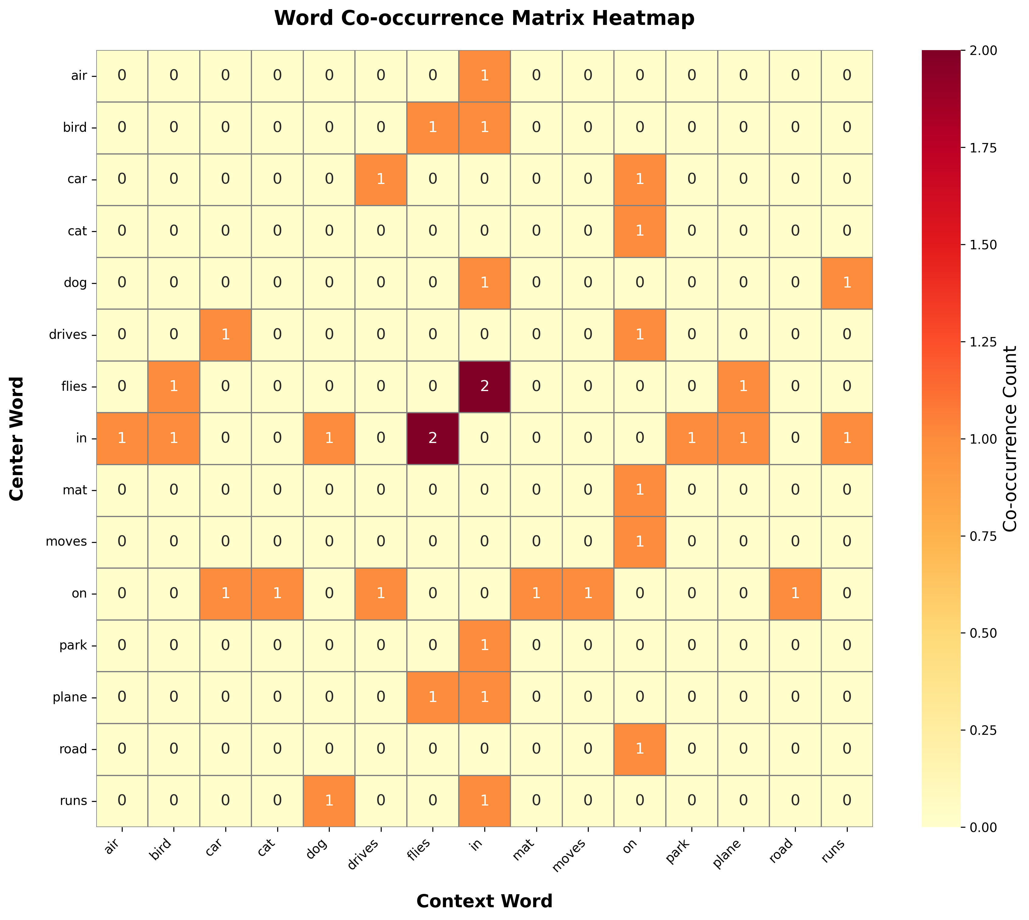
The heatmap reveals several important patterns. First, the matrix is sparse: most word pairs never co-occur (white cells with count 0). Second, semantically related words show similar patterns: "cat" and "dog" both have high co-occurrence with "the", "on", and "in", reflecting their similar grammatical roles. Third, the diagonal is empty because we don't count a word co-occurring with itself. These patterns are exactly what GloVe's matrix factorization captures: words with similar rows (or columns) in this matrix will have similar embeddings after training.

Even in this tiny example, we can see semantic clusters emerging. Words that appear in similar contexts will have similar rows (or columns) in the co-occurrence matrix, which translates to similar embeddings after factorization.

Now let's implement Word2Vec skip-gram with negative sampling from scratch. This implementation will help you understand exactly how embeddings are learned.

The Word2Vec class implements the skip-gram architecture with negative sampling. The embedding matrices are initialized with small random values, which will be updated during training. The embedding shape shows we have one vector per word in the vocabulary, with each vector having the specified embedding dimension.

Now let's train on a larger corpus. We'll use a simple text preprocessing pipeline and train for multiple epochs:

The vocabulary contains all unique words from our training corpus. We generate training pairs by sliding a context window across each sentence, creating (center word, context word) pairs. During training, the loss decreases as the model learns to predict context words more accurately. The decreasing loss indicates that the embeddings are learning meaningful relationships: words that appear in similar contexts are being pulled together in embedding space.

A loss curve shows how the model improves over training:

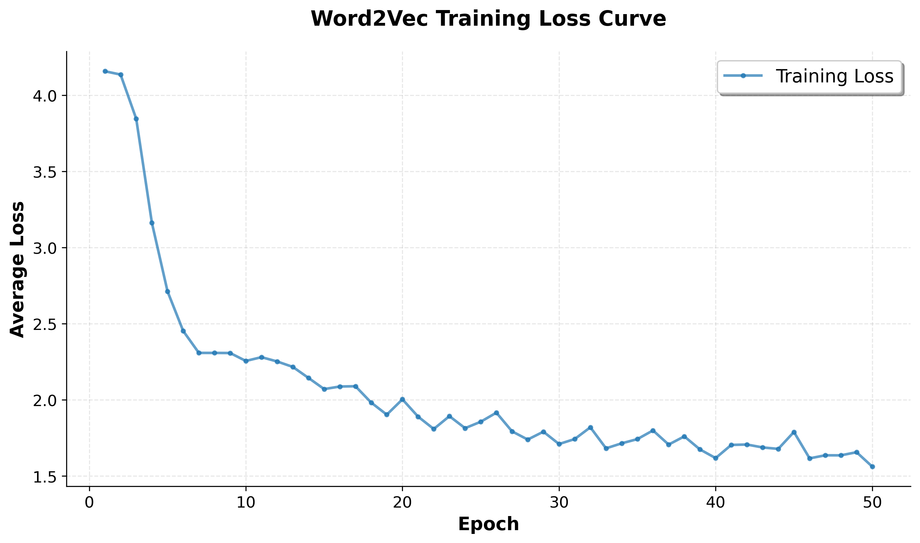
The loss curve demonstrates successful training: the loss decreases steadily from the initial random embeddings to a much lower value, indicating the model is learning meaningful word relationships. The initial rapid decrease shows the model quickly learns basic patterns, while the gradual decline and eventual plateau suggest it's converging to a stable solution where embeddings capture semantic relationships effectively.

Now let's visualize the embeddings to see if semantically similar words cluster together:

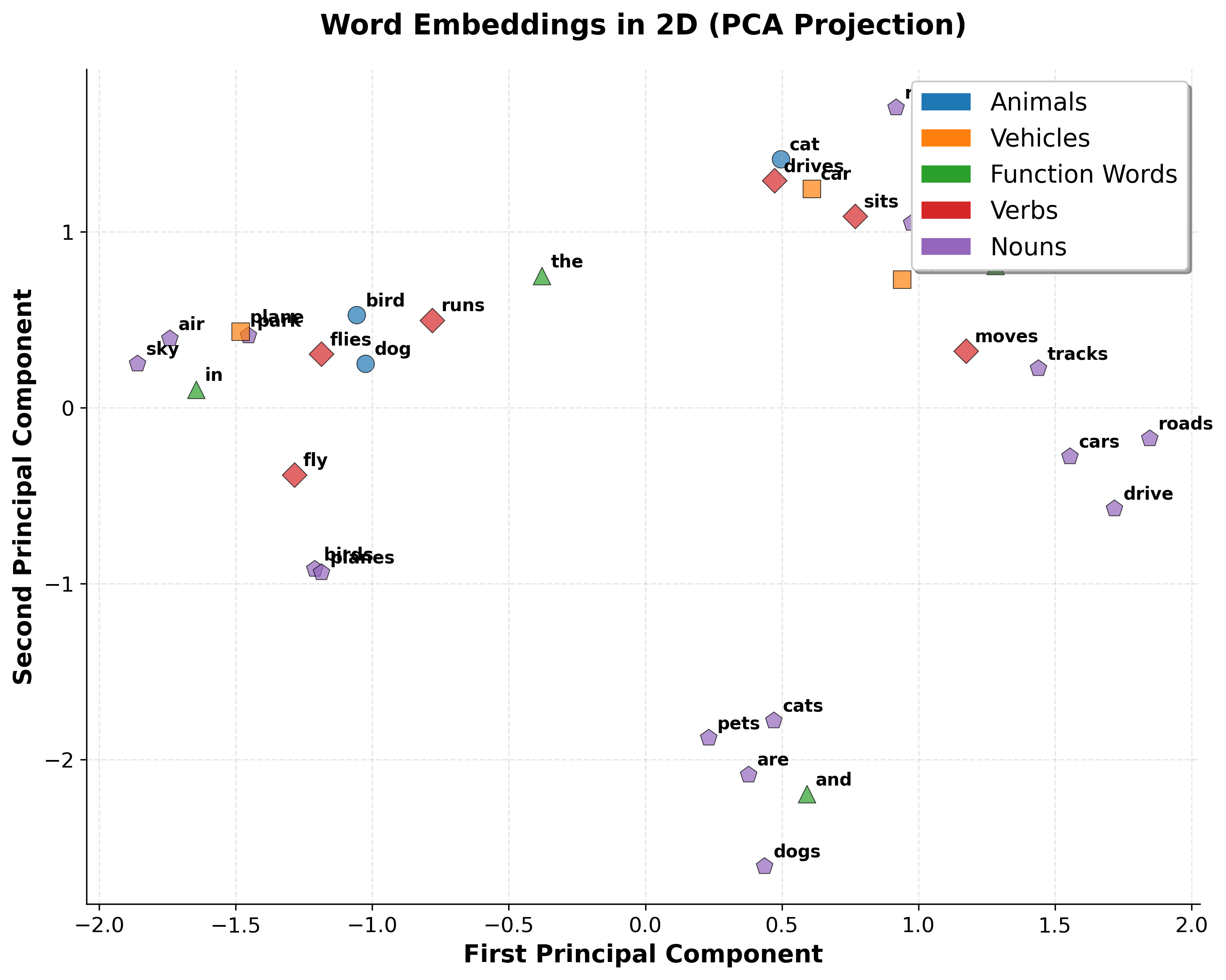
The visualization shows that even with minimal training data, Word2Vec learns meaningful structure. Animals cluster together, vehicles form their own group, and function words occupy a distinct region. This demonstrates how semantic relationships emerge naturally from co-occurrence patterns.

We can measure similarity between words using cosine similarity:

The similarity scores show how closely related words are in embedding space. Words with higher cosine similarity (closer to 1.0) have more similar embeddings, meaning they appear in similar contexts. For "cat", we expect to see other animals like "dog" or "bird" with high similarity. For "car", we expect vehicles like "plane" or "train". These results demonstrate that Word2Vec successfully captures semantic relationships: words that are semantically related have similar embeddings.

Word embeddings can capture analogies through vector arithmetic. The classic example is: "king - man + woman = queen". Let's test this:

Word analogies test whether embeddings capture relational patterns. The analogy "cat is to dog as car is to ?" asks: what word has the same relationship to "car" that "dog" has to "cat"? We expect "plane" or "train" (another vehicle). The vector arithmetic $\mathbf{v}_{\text{car}} + (\mathbf{v}_{\text{dog}} - \mathbf{v}_{\text{cat}})$ should point toward the answer. With our small vocabulary and limited training, results may not be perfect, but the principle demonstrates how embeddings encode relationships: semantic relationships become geometric relationships in vector space.

The Word2Vec implementation uses several key parameters that control training and embedding quality:

• embedding_dim (default: 100-300): The dimensionality of the embedding vectors. Larger dimensions can capture more nuanced relationships but require more training data and computation. Typical values range from 50-300, with 100-200 being most common for general-purpose embeddings.

• window_size (default: 5-10): The size of the context window on each side of the center word. Larger windows capture more global relationships (document-level patterns), while smaller windows focus on local syntactic relationships. For most applications, 5-10 words on each side works well.

• negative_samples (default: 5-20): The number of negative examples sampled for each positive example. More negative samples improve embedding quality but slow training. Values between 5-20 are typical, with 5-10 being common for large corpora.

• learning_rate (default: 0.01-0.05): The step size for gradient descent updates. Higher learning rates train faster but may overshoot optimal values. Lower learning rates are more stable but require more epochs. Start with 0.01-0.05 and adjust based on loss convergence.

• vocab_size: The number of unique words in the vocabulary. This is determined by your corpus and preprocessing choices. Larger vocabularies require more memory and computation but capture more word diversity.

These parameters interact: larger embedding dimensions and more negative samples improve quality but increase training time. For production use, start with moderate values (embedding_dim=200, window_size=5, negative_samples=5) and tune based on your specific task and computational constraints.

Both Word2Vec and GloVe produce high-quality embeddings, but they have different strengths:

Word2Vec advantages:

• Online learning: can process streaming data
• Memory efficient: doesn't need to store full co-occurrence matrix
• Fast training with negative sampling
• Better for very large corpora

GloVe advantages:

• Uses global statistics: all co-occurrence information simultaneously
• Often performs better on analogy tasks
• More interpretable: explicit relationship to co-occurrence statistics
• Can leverage pre-computed co-occurrence matrices

In practice, both methods produce embeddings of similar quality. The choice often depends on your specific constraints: use Word2Vec for streaming data or very large corpora, use GloVe when you can pre-compute co-occurrence statistics and want slightly better performance on semantic tasks.

Word embeddings revolutionized NLP, but they have important limitations that contextual embeddings (like BERT) address.

1. Static representations: Each word has a single embedding regardless of context. "bank" (financial institution) and "bank" (river edge) have the same vector, even though they mean different things.

2. Out-of-vocabulary words: Words not seen during training get no embedding. This is particularly problematic for morphologically rich languages and domain-specific terminology.

3. No sentence-level understanding: Embeddings capture word-level semantics but don't understand how words combine to form meaning. The phrase "not good" might be represented as the average of "not" and "good" embeddings, losing the negation.

4. Bias amplification: Embeddings learn biases present in training data. Gender stereotypes, racial biases, and other problematic associations get encoded in the vector space.

5. Limited to word-level: Can't represent subword units (important for morphologically rich languages) or multi-word expressions without special handling.

Despite these limitations, word embeddings had significant impact:

• Transfer learning: Pre-trained embeddings enabled NLP models to work with limited task-specific data
• Semantic search: Embeddings power modern search engines and recommendation systems
• Foundation for transformers: The embedding concept evolved into positional encodings and token embeddings in transformers
• Research catalyst: Sparked interest in representation learning that led to contextual embeddings

Word embeddings were a crucial stepping stone. They proved that dense vector representations could capture semantic relationships, setting the stage for contextual embeddings from transformers. Today, while static word embeddings are rarely used directly in state-of-the-art systems, the principles they established (dense representations, transfer learning, semantic relationships in vector space) remain foundational to modern NLP.

Word embeddings solve the fundamental problem of representing words as numbers in a way that captures semantic relationships. Unlike one-hot encoding, which treats all words as equally different, embeddings learn dense, low-dimensional vectors where similar words have similar representations.

Key takeaways:

• Distributional hypothesis: Words appearing in similar contexts have similar meanings. This principle underlies both Word2Vec and GloVe.

• Word2Vec: Learns embeddings by predicting context words (skip-gram) or center words (CBOW) using local windows. Negative sampling makes training efficient by approximating the expensive softmax.

• GloVe: Learns embeddings by factorizing a global co-occurrence matrix. Uses ratios of co-occurrence probabilities to capture word relationships.

• Semantic relationships: Embeddings encode meaning in vector geometry. Similarity is measurable (cosine similarity), and analogies can be solved through vector arithmetic.

• Limitations: Static representations can't handle polysemy, require handling of OOV words, and may encode biases from training data.

• Impact: Enabled transfer learning in NLP and laid the foundation for modern contextual embeddings.

Word embeddings transformed NLP by making semantic relationships computable. While superseded by contextual embeddings in most applications, understanding embeddings is important for grasping how modern language models represent and understand text.

Ready to test your understanding? Take this quick quiz to reinforce what you've learned about word embeddings, Word2Vec, and GloVe.