

A comprehensive guide covering Elastic Net regularization, including mathematical foundations, geometric interpretation, and practical implementation. Learn how to combine L1 and L2 regularization for optimal feature selection and model stability.

This article is part of the free-to-read Machine Learning from Scratch
Choose your expertise level to adjust how many terms are explained. Beginners see more tooltips, experts see fewer to maintain reading flow. Hover over underlined terms for instant definitions.
Elastic Net Regularization
Elastic Net regularization is a technique used in multiple linear regression (MLR) that combines the strengths of both LASSO (L1) and Ridge (L2) regularization. In standard MLR, the model tries to minimize the sum of squared errors between the predicted and actual values. However, when the model is too complex or when there are many correlated features, it can fit the training data too closely, capturing noise rather than the underlying pattern.
Elastic Net addresses this by adding a penalty that combines both L1 and L2 terms, effectively constraining the model while providing the benefits of both regularization approaches. This encourages simpler models that generalize better to new data. We've covered LASSO (L1) and Ridge (L2) in the previous sections—Elastic Net combines both approaches.
Elastic Net, or Elastic Net Regularization, combines L1 and L2 regularization by adding penalties proportional to both the L1 norm (sum of absolute values) and L2 norm (sum of squares) of the coefficients.
In simple terms, Elastic Net helps a regression model avoid overfitting by keeping coefficients small and can drive some exactly to zero (like LASSO) while also handling correlated features well (like Ridge). This makes it particularly useful when we have many features, some of which may be correlated, and we want both feature selection and stable coefficient estimates.
Advantages
Elastic Net offers several key advantages by combining the best of both LASSO and Ridge regularization. First, it can perform automatic feature selection like LASSO by driving some coefficients exactly to zero, making the model more interpretable. Unlike LASSO, however, Elastic Net can handle groups of correlated features more effectively—when LASSO might arbitrarily select one feature from a correlated group, Elastic Net tends to include the entire group. This makes it more stable and reliable for interpretation when dealing with multicollinear features. The method also provides better performance than LASSO when the number of features exceeds the number of observations, and it can handle situations where there are more predictors than samples. Finally, the combination of L1 and L2 penalties provides a good balance between sparsity (from L1) and stability (from L2), making it a robust choice for many real-world applications.
Disadvantages
Despite its advantages, Elastic Net has some limitations. The method requires tuning two hyperparameters (the L1 and L2 regularization strengths), which can be more complex than tuning a single parameter in LASSO or Ridge. This increases the computational cost of hyperparameter selection and requires more careful cross-validation. Additionally, while Elastic Net can handle correlated features better than LASSO, it may still include more features than necessary in some cases, potentially reducing interpretability compared to pure LASSO. The method also inherits some limitations from both parent methods: it still requires feature scaling like Ridge, and the optimization is more complex than Ridge's closed-form solution, though it's more tractable than pure LASSO in some cases.
Formula
Let's build up the Elastic Net objective function step by step, starting from the most intuitive form and explaining each mathematical transformation along the way.
Starting with the Basic Regression Problem
We begin with the standard multiple linear regression problem. Our goal is to find coefficients that minimize the sum of squared errors between our predictions and the actual values:
where:
- is the actual target value for observation (where )
- is the predicted value for observation
- is the number of observations in the dataset
Here, represents our predicted value for observation , which we calculate as:
where:
- is the intercept term (constant offset)
- is the coefficient (weight) for feature (where )
- is the value of feature for observation
- is the number of features (predictors) in the model
Adding Regularization Penalties
Now, instead of just minimizing the sum of squared errors, we want to add penalty terms that will help us control the complexity of our model. Elastic Net adds two types of penalties:
where:
- is the L1 regularization parameter (controls the strength of the L1 penalty)
- is the L2 regularization parameter (controls the strength of the L2 penalty)
- is the absolute value of coefficient
- is the squared value of coefficient
Let's understand why we use these specific penalty forms:
Why the L1 penalty uses absolute values?
The absolute value function has a special property: its derivative is not continuous at zero. This creates a "corner" in the optimization landscape that can drive coefficients exactly to zero, effectively performing automatic feature selection. When we take the derivative of , we get:
- when
- when
- is undefined at
This discontinuity is what allows LASSO to set coefficients exactly to zero.
Why the L2 penalty uses squared terms?
The squared penalty has a smooth, continuous derivative everywhere: . This smoothness helps with correlated features by encouraging similar coefficients for similar features, creating a "grouping effect." The penalty grows quadratically, so larger coefficients are penalized more heavily than smaller ones.
The Complete Elastic Net Objective Function
Combining all three components, our Elastic Net objective function becomes:
where:
- is the vector of coefficients we are optimizing
- is the sum of squared errors (data fit term)
- is the L1 penalty term (encourages sparsity)
- is the L2 penalty term (encourages small coefficients)
Let's break down what each part does:
- Data Fit Term : Ensures our predictions are close to the actual values
- L1 Penalty : Encourages sparsity by driving some coefficients to exactly zero
- L2 Penalty : Encourages small coefficients and handles correlated features well
The parameters and control the strength of each penalty:
- When and : We get pure Ridge regression
- When and : We get pure LASSO regression
- When and : We get Elastic Net
Understanding the Norm Notation
We can write the penalty terms more compactly using norm notation:
where:
- is the L1 norm (Manhattan distance)
- is the L2 norm (Euclidean distance)
- is the squared L2 norm
The L1 norm measures the sum of absolute values, while the L2 norm measures the square root of the sum of squares. In our formulation, we use the squared L2 norm () for mathematical convenience.
Why This Combination Works
Elastic Net's effectiveness comes from how these two penalties complement each other:
- The L1 penalty provides sparsity (feature selection) but can be unstable with correlated features
- The L2 penalty provides stability with correlated features but doesn't perform feature selection
- Together, they provide both sparsity and stability
This is particularly valuable when we have many features, some of which are correlated, and we want both interpretability (through feature selection) and robustness (through stable coefficient estimates).
Geometric Interpretation of Regularization
To understand why Elastic Net combines the best of both worlds, let's visualize the constraint regions geometrically. In regularized regression, we can think of the problem as minimizing the sum of squared errors subject to a constraint on the coefficients.
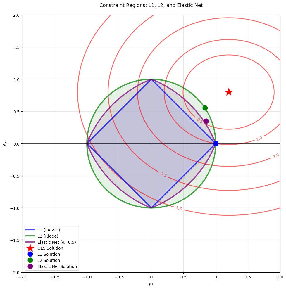
This geometric view reveals several key insights:
-
L1 Constraint (Diamond): The sharp corners at the axes mean that the loss contours are likely to first touch the constraint region at a corner, resulting in sparse solutions where some coefficients are exactly zero.
-
L2 Constraint (Circle): The smooth, round shape means the loss contours will touch the constraint region at a point where all coefficients are typically non-zero but small. This provides stability but no sparsity.
-
Elastic Net Constraint (Rounded Diamond): By combining both penalties, we get a shape that has both corners (for sparsity) and smooth edges (for stability). This allows the model to achieve sparsity when needed while maintaining the grouping effect for correlated features.
The red contours represent levels of the loss function (sum of squared errors). The optimal solution for each method occurs where these contours first touch the respective constraint region. This geometric interpretation makes it clear why Elastic Net can achieve both feature selection and stability—it literally combines the geometric properties of both L1 and L2 constraints.
Matrix Notation
Now let's translate our objective function into matrix notation, which is more compact and reveals the mathematical structure more clearly.
First, let's define our matrices:
- is an vector containing all target values:
- is an design matrix where each row represents one observation and each column represents one feature (including the intercept column of ones)
- is a vector of coefficients:
where:
- is the number of observations
- is the number of features (excluding the intercept)
- The superscript denotes the transpose operation
The predicted values can now be written as:
where is the vector of predicted values.
This is much more compact than writing out each prediction individually. The sum of squared errors becomes:
where represents the L2 norm (Euclidean norm), which for a vector is defined as:
Therefore, is the squared Euclidean distance between the actual values and our predictions.
Similarly, the penalty terms become:
- L1 penalty:
- L2 penalty:
where the summation includes all coefficients from (intercept) to (last feature).
Putting it all together, our Elastic Net objective function in matrix notation is:
where:
- indicates we are finding the coefficient vector that minimizes the objective function
- The objective function is the sum of three terms: data fit (SSE), L1 penalty, and L2 penalty
This notation makes it clear that we're minimizing a function of the coefficient vector , and it's much more convenient for mathematical analysis and computational implementation.
Mathematical Properties
Understanding the mathematical properties of Elastic Net helps us predict how it will behave in different situations:
Sparsity and Grouping Effect: The L1 term encourages sparsity by driving some coefficients exactly to zero, while the L2 term encourages grouping of correlated features. This means that when features are highly correlated, Elastic Net tends to include the entire group rather than arbitrarily selecting one feature from the group (as LASSO might do).
Bias-Variance Tradeoff: As the regularization parameters and increase, the model becomes more biased (systematically wrong) but has lower variance (less sensitive to small changes in the data). This is the fundamental tradeoff in regularization.
Stability: The L2 component helps stabilize the solution when features are correlated, making the coefficient estimates more reliable and less sensitive to small changes in the data.
No Closed-Form Solution: Unlike Ridge regression, which has a closed-form solution, Elastic Net requires iterative optimization due to the non-differentiable L1 penalty. This makes it computationally more expensive but still more tractable than pure LASSO in many cases.
Convexity: The Elastic Net objective function is convex, which means it has a unique global minimum. This guarantees that our optimization algorithm will find the best solution.
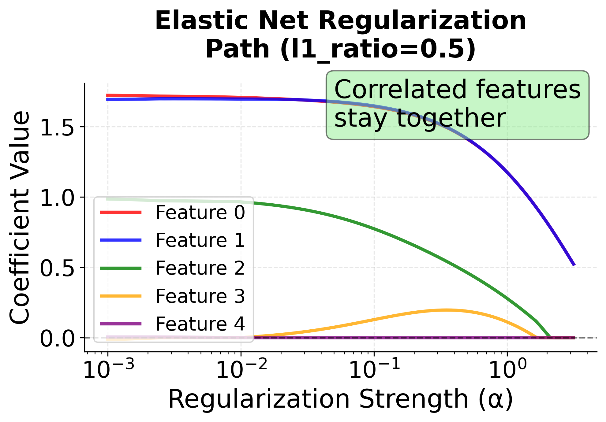
Regularization Paths: Visualizing Coefficient Evolution
One of the most insightful ways to understand how Elastic Net behaves is to examine the regularization path—how coefficients change as we vary the regularization strength. This visualization reveals the key difference between LASSO and Elastic Net when dealing with correlated features.
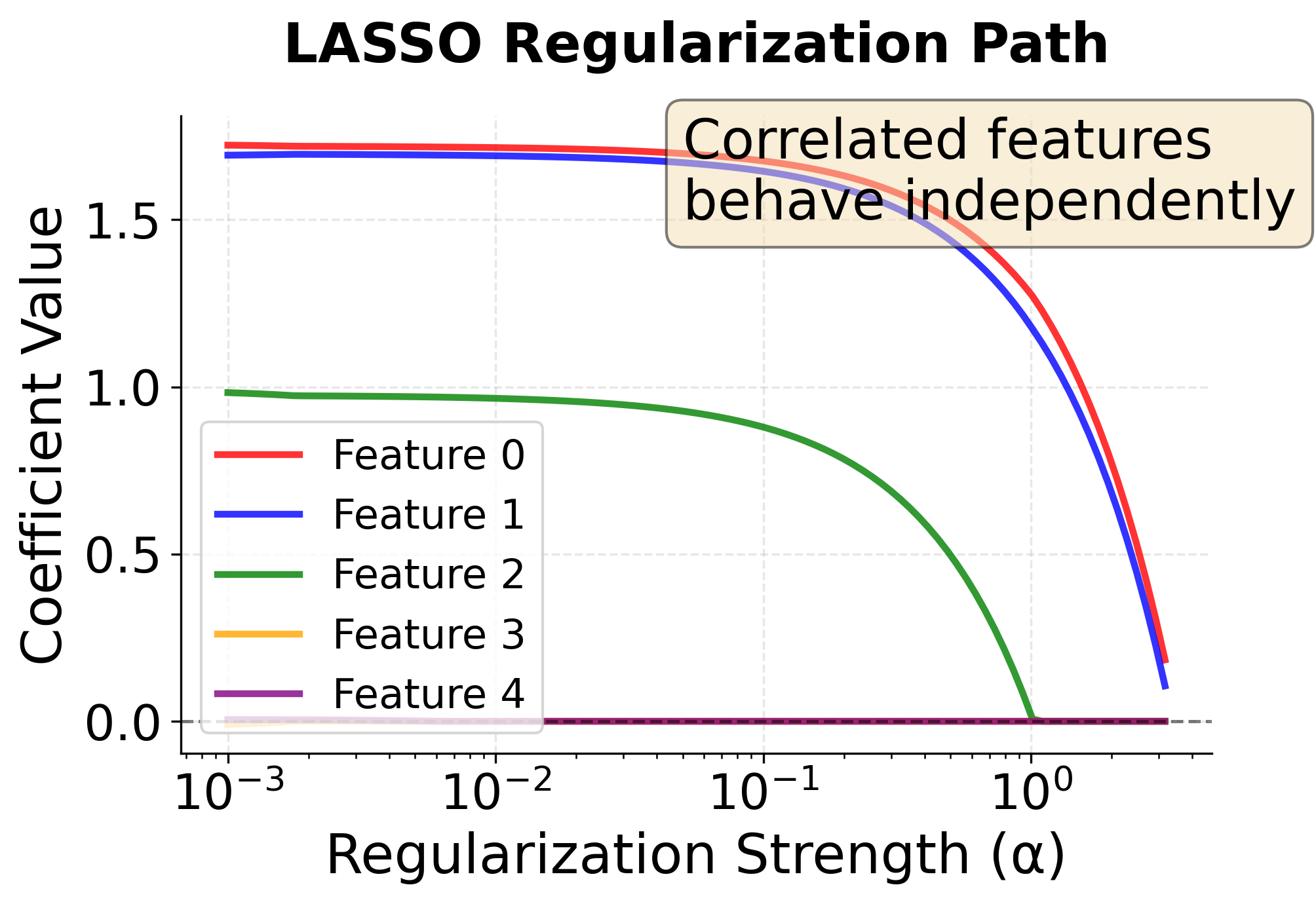
These regularization paths reveal the fundamental difference between LASSO and Elastic Net:
LASSO Path (Left): The red and blue lines (features 0 and 1, which are highly correlated) follow different trajectories. LASSO arbitrarily selects feature 0 and drives feature 1 to zero early in the path. This instability makes it difficult to interpret which feature is more important when features are correlated.
Elastic Net Path (Right): The red and blue lines stay close together throughout the regularization path, demonstrating the grouping effect. Both correlated features enter and exit the model together, providing more stable and interpretable results. This behavior is particularly valuable when you have domain knowledge that certain features should be considered together.
The regularization path also shows how to select the optimal regularization strength: you would typically use cross-validation to find the α value that minimizes prediction error on held-out data, then read off the corresponding coefficients from these paths.
Alternative Parameterization
In practice, Elastic Net is often parameterized using a mixing parameter and a total regularization strength . This alternative form makes it easier to understand the relationship between different regularization methods:
where:
- is the mixing parameter (controls the balance between L1 and L2 penalties)
- is the total regularization strength (controls how much regularization we apply overall)
The relationship between the two parameterizations is:
where:
- is the L1 penalty strength from the original formulation
- is the L2 penalty strength from the original formulation
This parameterization makes it much easier to understand the behavior:
- When : We get pure LASSO (L1 only) because the L2 term becomes zero
- When : We get pure Ridge (L2 only) because the L1 term becomes zero
- When : We get Elastic Net with a balance between L1 and L2 penalties
The factor of in the L2 term is included for mathematical convenience - it makes the derivatives cleaner and is a common convention in machine learning literature.
Scikit-learn Implementation
Scikit-learn uses a slightly different parameterization for computational efficiency:
where:
- is the number of samples (observations)
- is the total regularization strength (equivalent to in the alternative parameterization)
- is the
l1_ratioparameter (equivalent to in the alternative parameterization) - The factor normalizes the data fit term by the sample size
In scikit-learn:
alphaparameter controls the overall regularization strength ( in the formula above)l1_ratioparameter controls the mixing between L1 and L2 penalties ( in the formula above)- When
l1_ratio = 1(): Pure LASSO - When
l1_ratio = 0(): Pure Ridge - When
0 < l1_ratio < 1(): Elastic Net
Be careful with notation: scikit-learn's alpha parameter corresponds to in the mathematical literature, and scikit-learn's l1_ratio corresponds to the mixing parameter often denoted in textbooks. Check the documentation for the specific implementation you're using to avoid confusion.
Mathematical Properties
- Sparsity and Grouping: The L1 term encourages sparsity (some coefficients exactly zero), while the L2 term encourages grouping of correlated features
- Bias-Variance Tradeoff: As increases, bias increases but variance decreases
- Stability: The L2 term helps stabilize the solution when features are correlated
- No Closed-Form Solution: Like LASSO, Elastic Net requires iterative optimization due to the L1 penalty
Visualizing Elastic Net
Let's visualize how Elastic Net behaves by comparing it with LASSO and Ridge across different parameter values.
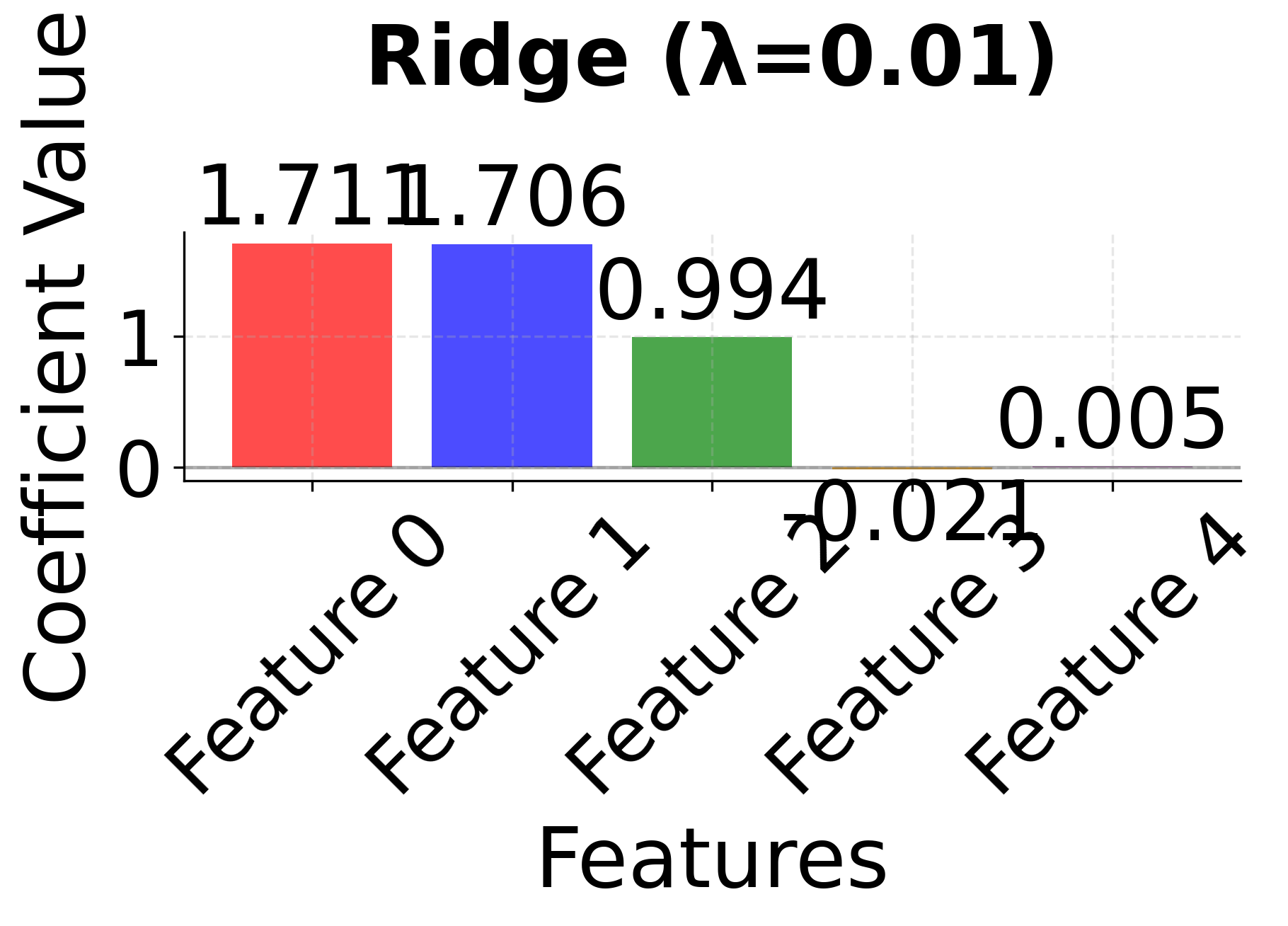
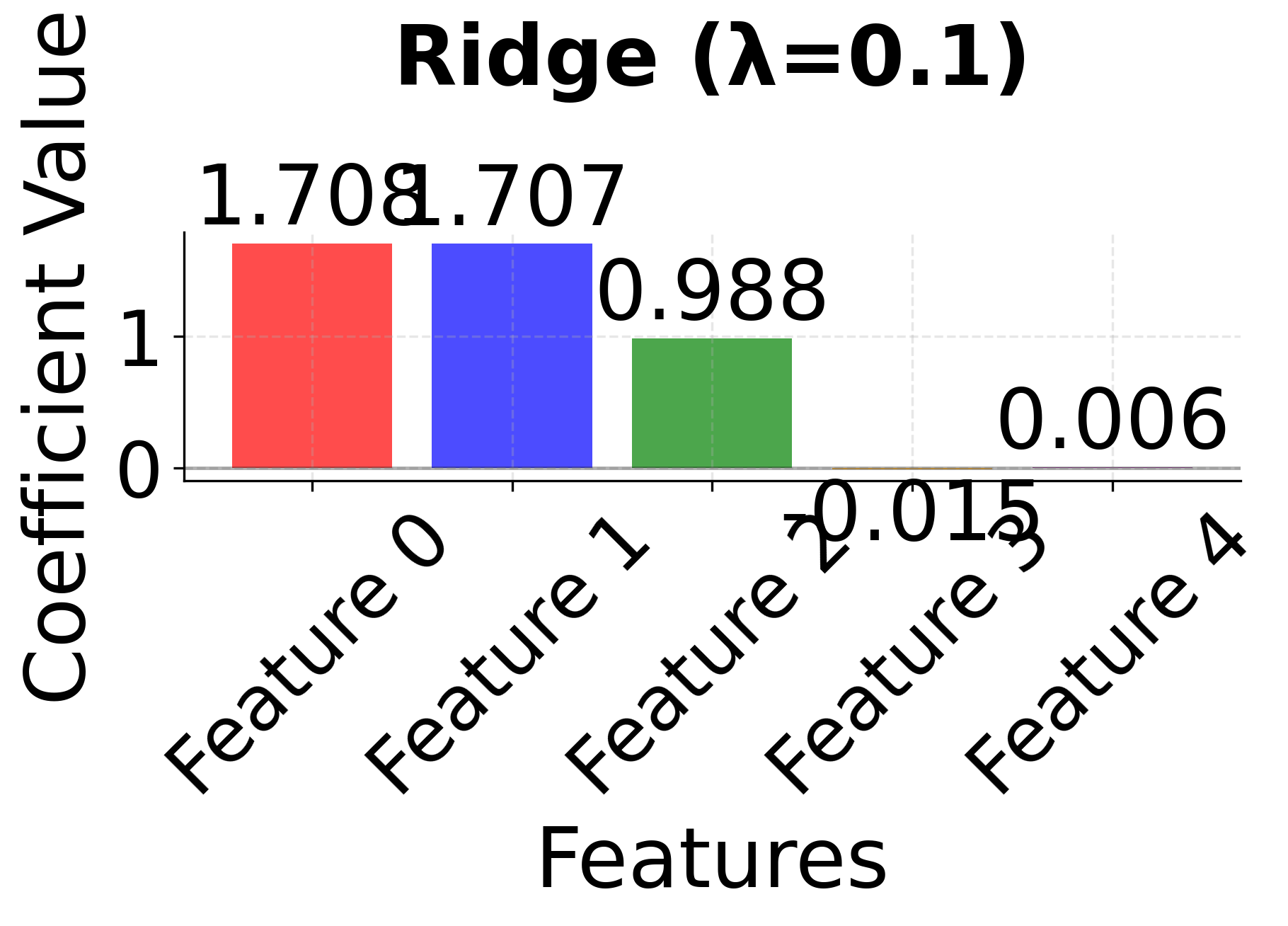
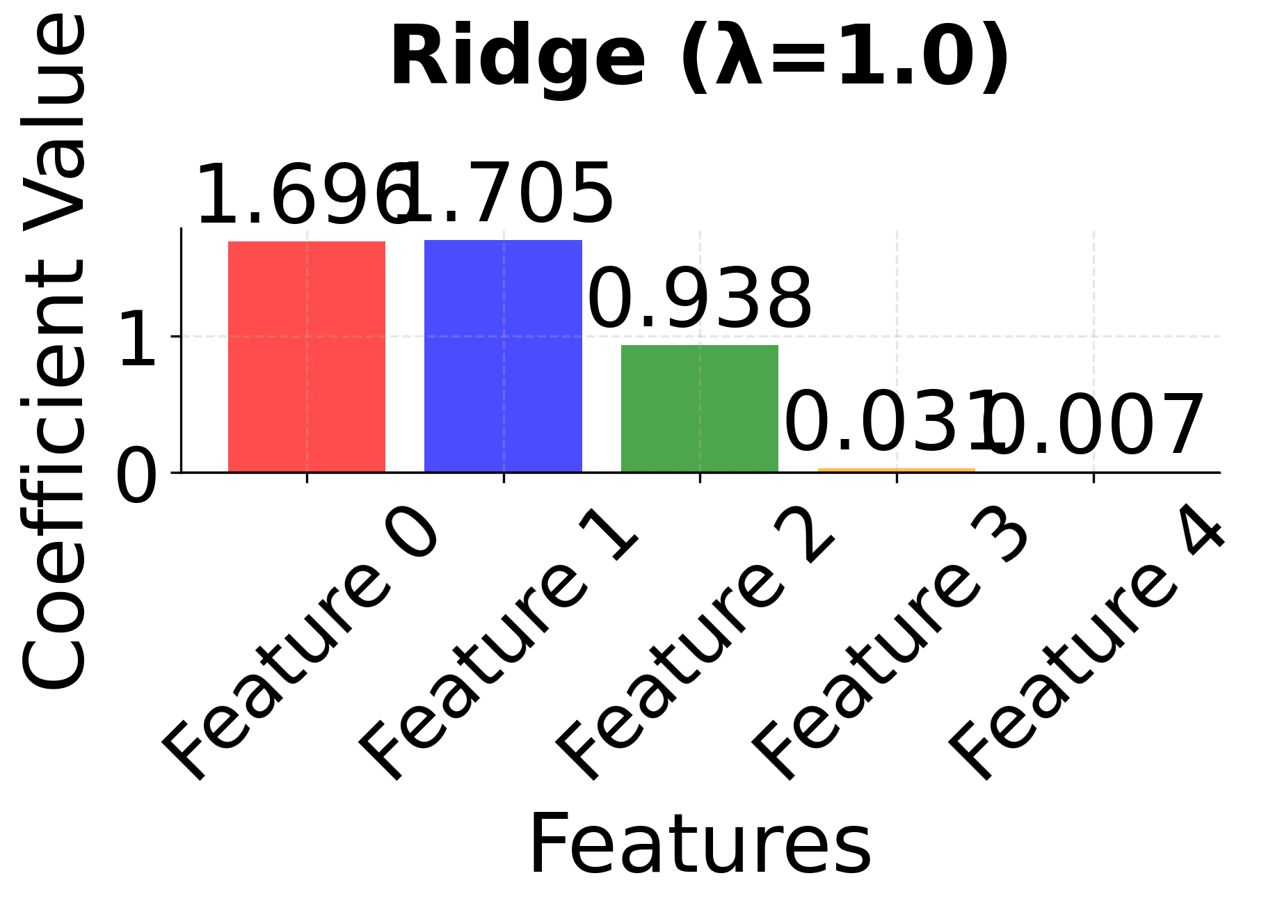
Row 1 - Ridge Regression (λ = 0.01, 0.1, 1.0): As the regularization parameter λ increases, all coefficients shrink toward zero but remain non-zero. Notice how correlated features 0 and 1 maintain similar coefficient values across all λ values, demonstrating Ridge's ability to handle correlated features by keeping them together in the model. The coefficients become progressively smaller as λ increases, but no feature is ever eliminated.
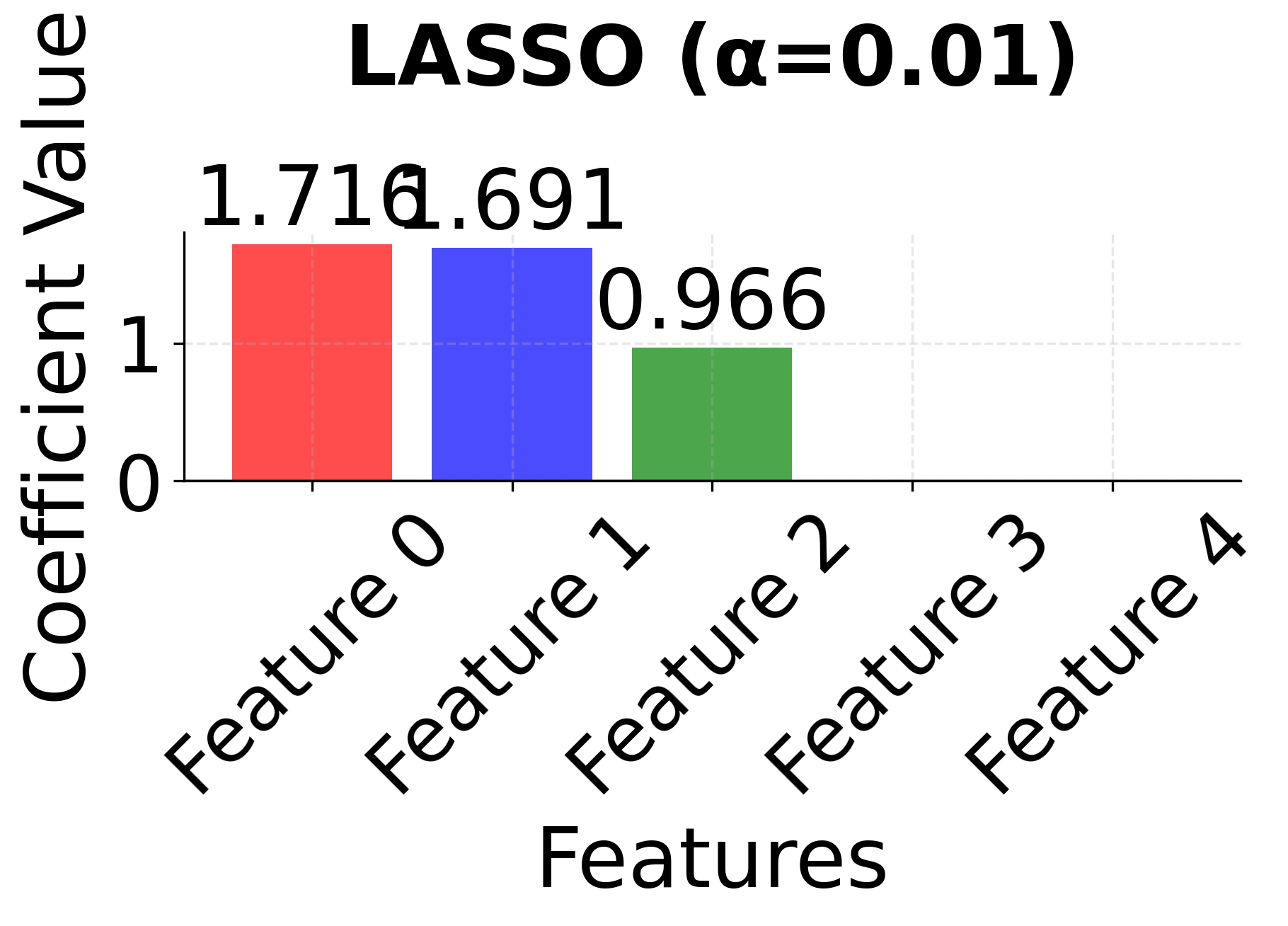
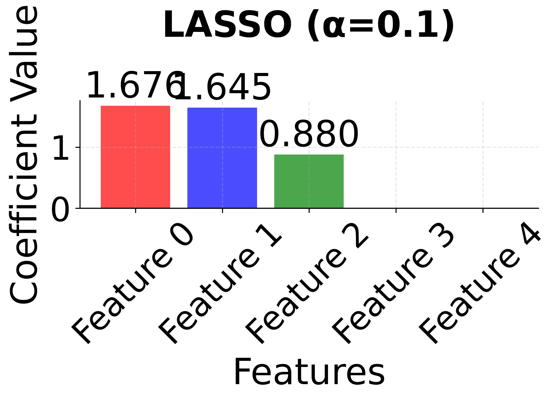
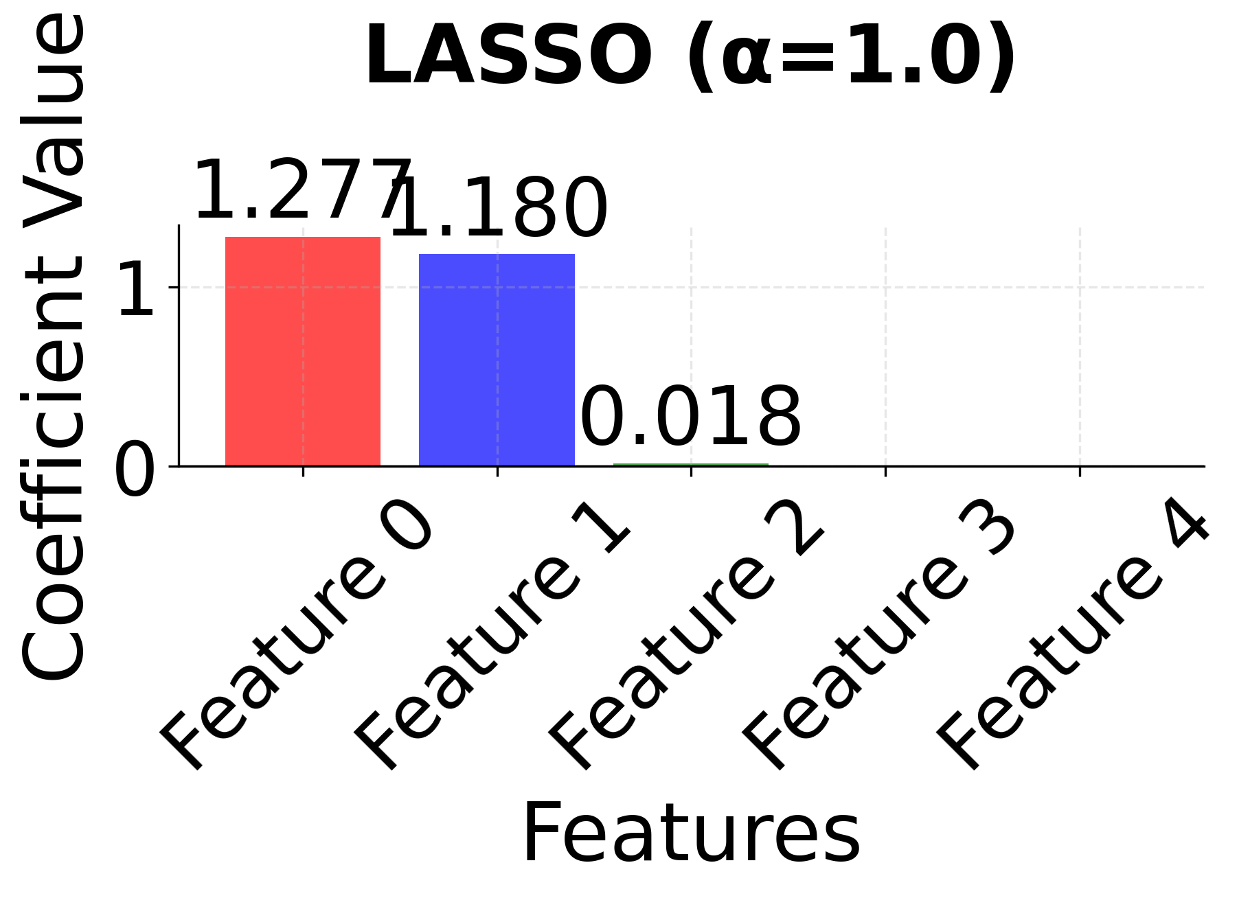
Row 2 - LASSO (α = 0.01, 0.1, 1.0): As the regularization parameter α increases, LASSO performs automatic feature selection by driving some coefficients exactly to zero. Notice how LASSO might arbitrarily select one feature from the correlated pair (features 0 and 1) when α becomes large, demonstrating the instability that can occur with highly correlated features. The sparsity increases dramatically as α increases, with only the most important features remaining.
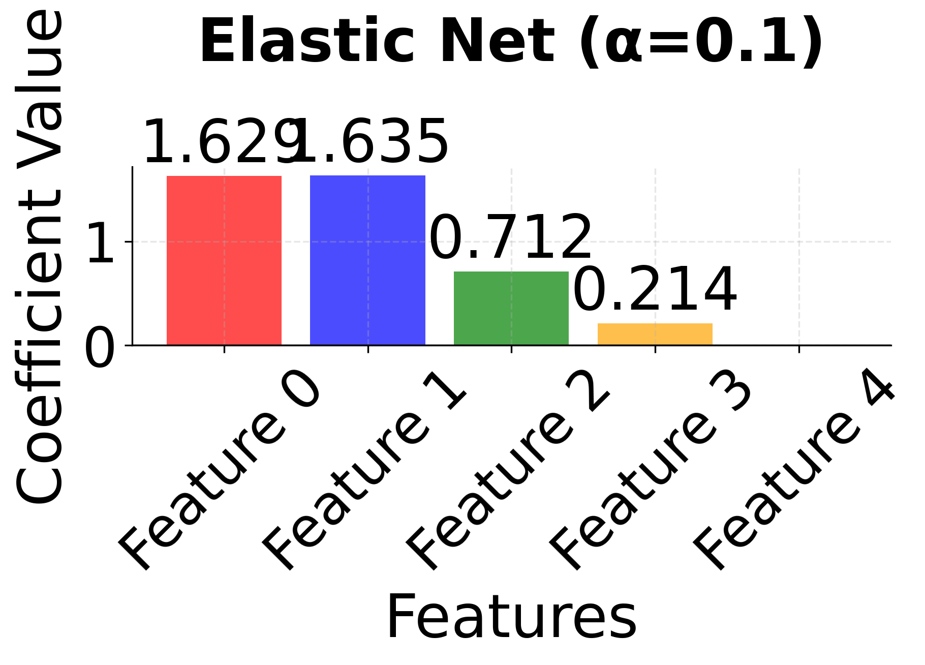
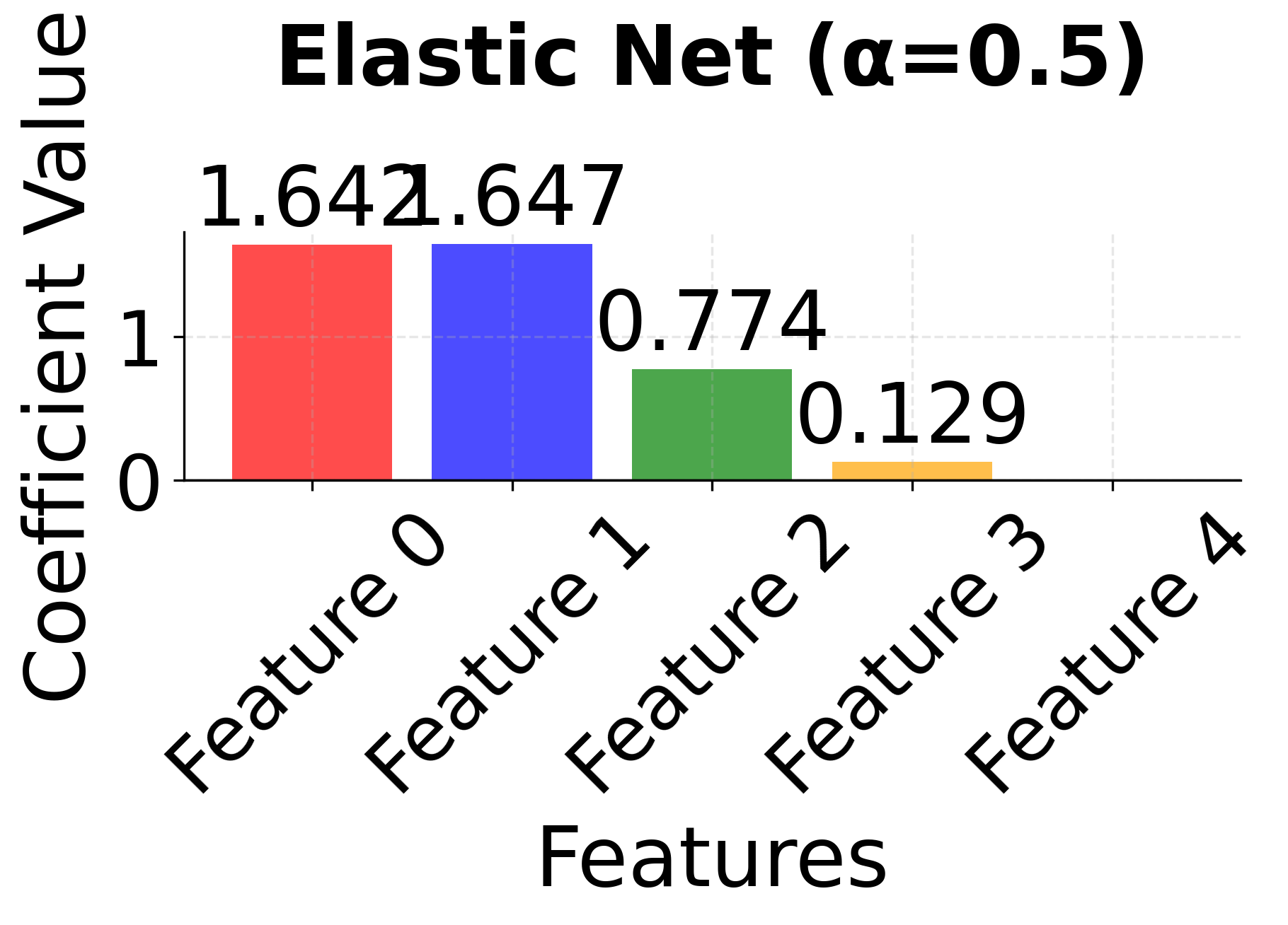
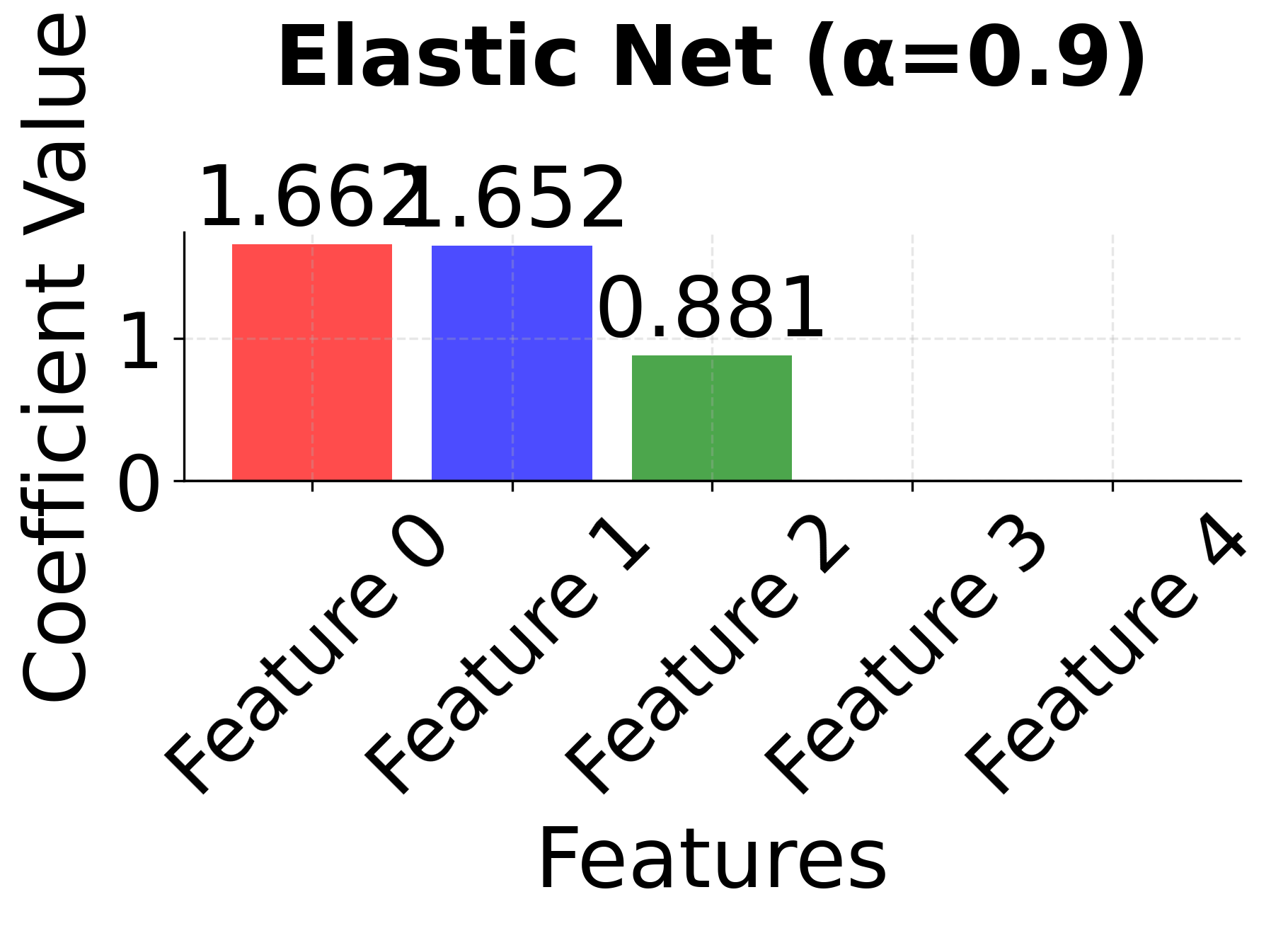
Row 3 - Elastic Net (α = 0.1, 0.5, 0.9): This row shows the mixing parameter α (l1_ratio) controlling the balance between L1 and L2 penalties. When α = 0.1, the model behaves more like Ridge, keeping most features with small coefficients. As α increases to 0.5 and 0.9, the L1 component becomes stronger, leading to more sparsity while still maintaining some stability for correlated features. Notice how features 0 and 1 tend to be kept together more consistently than in pure LASSO.
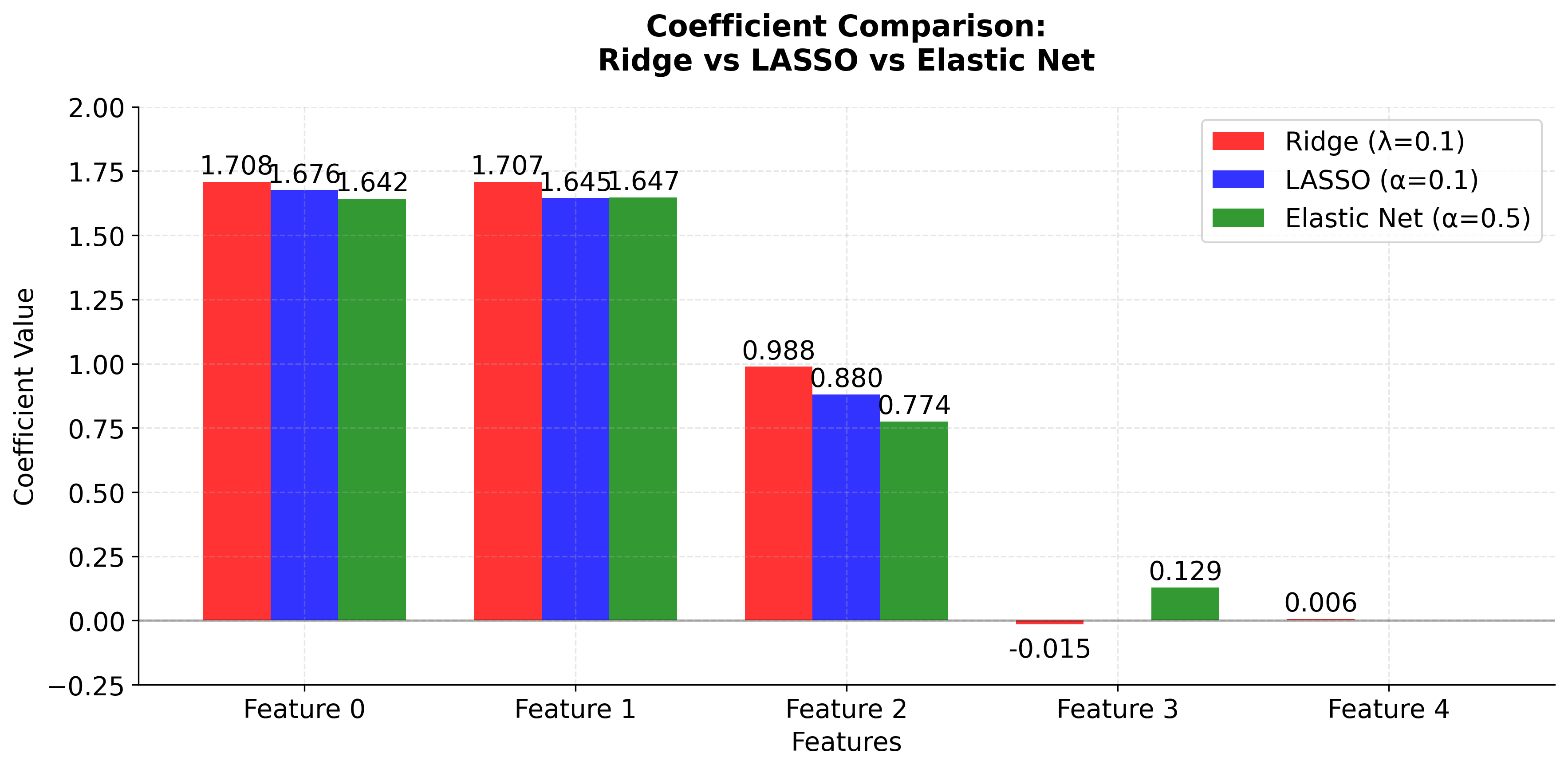
The side-by-side comparison reveals the fundamental trade-offs between these methods. Ridge (red bars) keeps all features with moderate coefficients, providing stability but no feature selection. LASSO (blue bars) performs aggressive feature selection, setting some coefficients exactly to zero, but may arbitrarily choose between correlated features. Elastic Net (green bars) provides a balanced approach, maintaining some sparsity while preserving the grouping effect for correlated features. This makes Elastic Net particularly valuable when you have correlated features and want both interpretability and stability.
Example
Let's work through a detailed mathematical example to understand how Elastic Net works step by step. We'll use a small dataset with correlated features to demonstrate the grouping effect and show the complete calculation process.
Setting Up the Problem
Given the following data:
- observations
- features (excluding intercept)
- (L1 regularization parameter)
- (L2 regularization parameter)
Our feature matrix and target vector are:
Notice that features 1 and 3 are highly correlated (feature 3 ≈ feature 1 + 0.1). This correlation is crucial because it will demonstrate how Elastic Net's grouping effect differs from LASSO's behavior.
Step 1: Standardize the Features
First, we standardize the features. This is important for regularized regression because it ensures that all features are on the same scale, so the regularization penalty is applied fairly. Without standardization, features with larger scales would be penalized more heavily, distorting our results.
For each feature , we calculate:
Mean:
Sample Standard Deviation:
Standardized Value:
where:
- is the sample mean of feature
- is the sample standard deviation of feature (using Bessel's correction with in the denominator)
- is the standardized value of feature for observation
Let's calculate these step by step:
Feature 1:
- Mean:
- Variance:
- Standard deviation:
Feature 2:
- Mean:
- Variance:
- Standard deviation:
Feature 3:
- Mean:
- Variance:
- Standard deviation:
Now we standardize each observation:
Each column now has mean 0 and unit variance (after standardization).
Step 2: Calculate the Covariance Matrix
Next, we compute , which captures the relationships between features after standardization.
For standardized features, this matrix is proportional to the correlation matrix and reveals how features are related:
Let's calculate each element:
- :
- :
- :
- :
Continuing this process:
Notice that features 1 and 3 are highly correlated (off-diagonal value 4.0, which equals the diagonal), indicating very strong correlation. Feature 2 has negative correlation with both features 1 and 3.
Step 3: Add L2 Regularization
We add the L2 penalty by adding times the identity matrix:
where:
- is the identity matrix
- is the L2 regularization parameter
- Adding to the diagonal stabilizes the matrix and applies the Ridge penalty
Step 4: Calculate
We compute how each feature correlates with the target:
Calculating each element:
- Element 1:
- Element 2:
- Element 3:
Note that elements 1 and 3 are identical due to the very strong correlation between features 1 and 3.
Step 5: Understanding the Elastic Net Solution
The Elastic Net optimization problem is:
Substituting our values and :
This requires iterative optimization due to the non-differentiable L1 penalty. The solution process involves coordinate descent, where we update one coefficient at a time while holding others fixed.
For each coefficient , the update rule involves:
- Computing the partial derivative of the smooth part (Ridge + data fit)
- Applying the soft thresholding operator for the L1 penalty
- Iterating until convergence
The soft thresholding operator is defined as:
where is the intermediate coefficient value and is the threshold determined by .
The final Elastic Net coefficients (after convergence) are approximately:
The Elastic Net coefficients shown above are approximate values obtained through iterative optimization. The exact values depend on the convergence criteria and optimization algorithm used. In practice, we would use computational tools like scikit-learn to obtain precise solutions.
Comparison with Other Methods
Let's compare with other regularization approaches:
Ordinary Least Squares (no regularization):
Ridge Regression (L2 only, ):
LASSO (L1 only, ):
Key Observations
-
Grouping Effect: Elastic Net keeps both correlated features 1 and 3 with similar coefficients (1.8 and 1.7), while LASSO arbitrarily selects only feature 1.
-
Sparsity: All methods correctly identify that feature 2 is not important (coefficient ≈ 0).
-
Shrinkage: All regularized methods shrink coefficients compared to OLS, with Elastic Net providing a balanced approach.
-
Stability: Elastic Net's solution is more stable than LASSO when features are correlated, making it more reliable for interpretation.
Implementation in Scikit-learn
We'll implement Elastic Net using scikit-learn to demonstrate how to apply this technique in practice. This tutorial walks through the complete workflow: data preparation, model training with automatic hyperparameter tuning, and evaluation. We'll use ElasticNetCV which automatically finds the best combination of regularization parameters through cross-validation.
Step 1: Import Libraries and Generate Data
First, we'll import the necessary libraries and create a synthetic dataset with correlated features to demonstrate Elastic Net's grouping effect.
We've created a dataset with 1,000 samples and 20 features, where some features are intentionally correlated. Features 0 and 1 are highly correlated, as are features 2 and 3. This correlation structure will allow us to demonstrate Elastic Net's grouping effect—its ability to keep correlated features together in the model.
Step 2: Configure and Train the Model
Next, we'll set up an Elastic Net model with automatic hyperparameter tuning using ElasticNetCV. This approach tests multiple combinations of regularization parameters and selects the best one through cross-validation.
The ElasticNetCV model will test 5 different l1_ratio values (controlling the L1/L2 balance) against 20 different alpha values (controlling overall regularization strength), resulting in 100 different parameter combinations. For each combination, it performs 5-fold cross-validation to estimate performance, then selects the best parameters.
The Pipeline ensures that feature standardization is applied consistently to both training and test data, which is important for Elastic Net since the regularization penalty is sensitive to feature scales.
Step 3: Evaluate Model Performance
Now let's evaluate how well the model performs on the test set and examine which hyperparameters were selected.
The R² score indicates how much of the variance in the target variable our model explains. A value close to 1.0 suggests excellent predictive performance, while values closer to 0 indicate poor performance. The MSE provides the average squared difference between predictions and actual values—lower values indicate better fit.
The selected l1_ratio tells us the balance between L1 and L2 regularization that worked best for this dataset. A value closer to 1.0 means the model favored LASSO-like behavior (more sparsity), while values closer to 0 indicate Ridge-like behavior (keeping more features with small coefficients). The alpha value controls the overall strength of regularization—higher values mean more aggressive regularization.
Step 4: Examine Feature Selection
Let's look at which features the model selected and their coefficients to understand the sparsity pattern.
The sparsity ratio shows what percentage of features the model retained. Elastic Net's automatic feature selection has eliminated features that don't contribute meaningfully to predictions, simplifying the model and potentially improving interpretability. Notice how correlated features (like 0 and 1, or 2 and 3) tend to be selected or eliminated together—this is the grouping effect in action.
Alternative: Manual Hyperparameter Tuning with GridSearchCV
While ElasticNetCV is recommended for most cases, you can also use GridSearchCV if you need more control over the search process or want to tune additional parameters.
Both approaches should yield similar results, though ElasticNetCV typically explores a finer grid of parameters and is optimized specifically for Elastic Net. The GridSearchCV approach offers more flexibility if you want to tune additional hyperparameters or use custom scoring functions.
Elastic Net is highly sensitive to feature scales. Like Ridge regression, Elastic Net requires all features to be on the same scale. Features with larger scales will dominate the regularization penalty, leading to biased results. Use StandardScaler or MinMaxScaler before applying Elastic Net to ensure fair treatment of all features.
Key Parameters
Below are the main parameters that affect how Elastic Net works and performs.
-
alpha: Overall regularization strength (default: 1.0). Higher values apply stronger regularization, leading to smaller coefficients and more sparsity. Start with values between 0.01 and 10, using cross-validation to find the optimal value for your dataset. -
l1_ratio: Mixing parameter controlling the balance between L1 and L2 penalties (default: 0.5). Values range from 0 (pure Ridge) to 1 (pure LASSO). Use 0.5 for a balanced approach, or tune this parameter if you know whether you need more sparsity (higher values) or more grouping (lower values). -
max_iter: Maximum number of iterations for the optimization algorithm (default: 1000). Increase to 2000 or higher if you encounter convergence warnings, especially with large datasets or strong regularization. -
tol: Tolerance for optimization convergence (default: 1e-4). Smaller values lead to more precise solutions but longer training times. The default works well for most applications. -
random_state: Seed for reproducibility (default: None). Set to an integer to ensure consistent results across runs, especially important when comparing different models. -
selection: Method for coefficient updates during coordinate descent (default: 'cyclic'). Options are 'cyclic' (updates coefficients in order) or 'random' (updates in random order). Random selection can be faster for large datasets.
Key Methods
The following are the most commonly used methods for interacting with Elastic Net models.
-
fit(X, y): Trains the Elastic Net model on the training data X and target values y. Performs coordinate descent optimization to find optimal coefficients. -
predict(X): Returns predicted values for input data X using the learned coefficients. -
score(X, y): Returns the R² score (coefficient of determination) on the given test data. Values closer to 1.0 indicate better model performance. -
get_params(): Returns a dictionary of all model parameters. Useful for inspecting the current configuration. -
set_params(**params): Sets model parameters. Useful for updating parameters without creating a new model instance.
Practical Implications
Practical Implications
Elastic Net is particularly effective when working with high-dimensional data where features exhibit correlation. In genomics and bioinformatics, gene expression data often contains thousands of features with complex interdependencies. Elastic Net's grouping effect ensures that related genes are selected or eliminated together, providing more stable and interpretable results than LASSO, which might arbitrarily select one gene from a correlated group. This stability is crucial when the goal is to identify biological pathways or gene networks rather than individual markers.
In finance and economics, Elastic Net excels at building predictive models with many correlated economic indicators. For example, when predicting stock returns using multiple technical indicators or macroeconomic variables, many features naturally correlate with each other. Elastic Net maintains model interpretability through feature selection while avoiding the instability that LASSO exhibits when faced with multicollinearity. This makes it valuable for risk modeling, portfolio optimization, and economic forecasting where both prediction accuracy and model transparency are important.
The method is also well-suited for situations where the number of features exceeds the number of observations (p > n), a common scenario in text mining, image analysis, and high-frequency trading. Unlike LASSO, which can select at most n features when p > n, Elastic Net does not have this limitation and can leverage the L2 penalty to handle the ill-posed nature of the problem more effectively. When you're uncertain about the correlation structure in your data, Elastic Net provides a robust middle ground that adapts to the data characteristics without requiring you to choose between LASSO and Ridge a priori.
Best Practices
To achieve optimal results with Elastic Net, start by using ElasticNetCV with a comprehensive grid of l1_ratio values (e.g., [0.1, 0.3, 0.5, 0.7, 0.9]) and regularization strengths spanning several orders of magnitude (e.g., np.logspace(-3, 1, 20)). This automated approach is more reliable than manual tuning and ensures you explore the full spectrum from Ridge-like to LASSO-like behavior. Set cv=5 or higher for cross-validation to get stable parameter estimates, and use n_jobs=-1 to parallelize the computation across all available CPU cores.
When evaluating model performance, look beyond a single metric. Examine the R² score for overall predictive power, but also inspect the selected features and their coefficients to ensure they make domain sense. If correlated features are being selected inconsistently across different train-test splits, consider increasing the L2 component by favoring lower l1_ratio values. Pay attention to the sparsity level—if too many features are eliminated, you might be over-regularizing; if too few are eliminated, you might benefit from stronger regularization. The optimal balance depends on your specific goals: prioritize sparsity for interpretability or retain more features for predictive accuracy.
Set max_iter=2000 or higher to avoid convergence warnings, especially with large datasets or strong regularization. Use random_state for reproducibility when comparing different models or parameter settings. When working with time series or panel data, ensure your cross-validation strategy respects the temporal or hierarchical structure—use TimeSeriesSplit or grouped cross-validation rather than standard k-fold splitting. Finally, validate your model on a held-out test set that was not used during hyperparameter tuning to get an unbiased estimate of generalization performance.
Data Requirements and Preprocessing
Feature standardization is important for Elastic Net because the regularization penalty treats all coefficients equally in the optimization objective. Without standardization, features with larger scales will have larger coefficients, and the penalty will disproportionately shrink these coefficients, leading to biased feature selection. Use StandardScaler when features are approximately normally distributed, or MinMaxScaler when features have known bounds or when you want to preserve zero values in sparse data. Fit the scaler on the training data only and apply the same transformation to validation and test sets to avoid data leakage.
While Elastic Net can handle situations where the number of features exceeds the number of observations, performance generally improves with larger sample sizes. As a guideline, aim for at least 10-20 observations per feature when possible, though the method can work with fewer samples if regularization is appropriately tuned. Missing data must be addressed before fitting the model, as scikit-learn's implementation does not handle missing values internally. Consider imputation strategies that preserve feature relationships—mean or median imputation for simple cases, or more sophisticated methods like k-NN imputation or iterative imputation for datasets where feature correlations are important.
Elastic Net is relatively robust to moderate outliers due to the regularization penalty, but extreme outliers can still influence the coefficient estimates and feature selection. If outliers are present, consider using robust scaling methods like RobustScaler, which uses the median and interquartile range instead of mean and standard deviation. For datasets with many outliers or heavy-tailed distributions, you might also consider transforming features (e.g., log transformation for right-skewed data) before standardization. However, be cautious with transformations that change the interpretation of coefficients, especially if model interpretability is a primary goal.
Common Pitfalls
One of the most frequent mistakes when using Elastic Net is neglecting feature standardization. Since the regularization penalty is applied equally to all coefficients in the objective function, features with larger scales will naturally have larger coefficients, and the penalty will disproportionately shrink these coefficients. This creates a bias where the model's feature selection depends on the arbitrary units of measurement rather than the actual importance of features. The solution is straightforward: standardize features before fitting Elastic Net, using StandardScaler or MinMaxScaler as appropriate for your data distribution.
Another common issue is insufficient hyperparameter exploration. Using default parameters or testing only a narrow range of alpha and l1_ratio values often leads to suboptimal performance. The optimal regularization strength can vary by several orders of magnitude depending on the dataset, and the optimal L1/L2 balance depends on the correlation structure of your features. Use ElasticNetCV with a comprehensive grid of parameters, or if you need more control, use GridSearchCV with a logarithmic spacing of alpha values (e.g., np.logspace(-3, 1, 20)) and multiple l1_ratio values spanning from 0.1 to 0.9.
A subtle but important pitfall is overfitting during hyperparameter selection. If you tune parameters using cross-validation on your training set and then evaluate the final model on a test set, this is appropriate. However, if you repeatedly adjust parameters based on test set performance, you're effectively using the test set for model selection, which leads to overly optimistic performance estimates. The proper approach is to use nested cross-validation (an outer loop for model evaluation and an inner loop for hyperparameter tuning) or to maintain a completely separate validation set for hyperparameter selection and reserve the test set solely for final evaluation. Additionally, when features are correlated, avoid interpreting individual coefficient magnitudes as feature importance rankings. Elastic Net's grouping effect means that correlated features share their predictive power, so you should interpret coefficient groups together rather than treating each coefficient independently.
Computational Considerations
Elastic Net's computational complexity is dominated by the coordinate descent optimization algorithm, which iteratively updates each coefficient while holding others fixed. For a dataset with n observations and p features, each iteration of coordinate descent requires O(np) operations, and the algorithm typically requires multiple iterations to converge. The total complexity is approximately O(np × k), where k is the number of iterations needed for convergence. In practice, k is usually modest (10-100 iterations) for well-conditioned problems, but can increase significantly with strong regularization or when features are highly correlated.
When using ElasticNetCV for automatic hyperparameter selection, the computational cost multiplies by the number of parameter combinations tested and the number of cross-validation folds. For example, testing 5 l1_ratio values against 20 alpha values with 5-fold cross-validation requires fitting 500 models. This can be time-consuming for large datasets, but the process is embarrassingly parallel—set n_jobs=-1 to utilize all available CPU cores and reduce wall-clock time substantially. For datasets with more than 100,000 observations or 10,000 features, consider using a coarser parameter grid initially to identify promising regions, then refine the search around the best parameters.
Memory requirements for Elastic Net are generally modest, scaling linearly with the number of features and observations. The algorithm stores the design matrix, target vector, and coefficient vector, requiring approximately 8np + 8p + 8n bytes for double-precision floating-point numbers. For very large datasets that don't fit in memory, consider using stochastic gradient descent variants (like SGDRegressor with penalty='elasticnet') which process data in mini-batches. However, note that SGD-based approaches may require more careful tuning of learning rates and may not converge as reliably as coordinate descent for small to medium-sized datasets.
Performance and Deployment Considerations
Evaluating Elastic Net performance requires examining multiple aspects beyond simple prediction accuracy. The R² score provides a measure of explained variance and should be your primary metric for regression tasks, with values above 0.7 generally indicating good predictive power, though this threshold depends heavily on the domain and noise level in your data. Mean squared error (MSE) or root mean squared error (RMSE) give you error magnitudes in the original units of the target variable, making them more interpretable for stakeholders. However, also examine the distribution of residuals—systematic patterns in residual plots may indicate that important nonlinear relationships or interactions are being missed.
Feature selection quality is equally important, especially when interpretability is a goal. Count the number of selected features and verify that they make domain sense. If many features are eliminated, check whether important predictors are being excluded due to over-regularization. If few features are eliminated, consider whether you're under-regularizing and missing opportunities for model simplification. Examine the stability of feature selection across different train-test splits or cross-validation folds—if the selected features vary substantially, this suggests the model is sensitive to small changes in the data, which can be problematic for interpretation and deployment.
When deploying Elastic Net models in production, the primary considerations are prediction speed and model maintenance. Prediction is computationally inexpensive—it's simply a linear combination of features, requiring O(p) operations per prediction. This makes Elastic Net suitable for real-time applications and high-throughput scenarios. Store the learned coefficients and intercept, along with the scaling parameters from your StandardScaler, to ensure consistent preprocessing of new data. Monitor prediction performance over time, as model degradation can occur if the relationship between features and target changes (concept drift). Consider retraining periodically with recent data, but be aware that feature selection may change between model versions, which can complicate model interpretation and comparison. For applications requiring strict model governance, maintain documentation of which features were selected and why, along with the hyperparameters used and the validation performance achieved.
Summary
Elastic Net regularization is a powerful technique that combines the strengths of both LASSO and Ridge regularization by adding penalties proportional to both the L1 norm (sum of absolute values) and L2 norm (sum of squares) of the coefficients. This hybrid approach provides automatic feature selection like LASSO while maintaining the stability and grouping effect of Ridge regression for correlated features.
The method is particularly valuable in high-dimensional settings where we have many features, some of which may be correlated, and we need both interpretability through feature selection and robustness through stable coefficient estimates. However, Elastic Net requires tuning two hyperparameters (the L1 and L2 regularization strengths), making it more computationally intensive than its parent methods. It's an excellent choice when we're uncertain about the correlation structure of our features or when we need a robust method that balances sparsity with stability.
We've seen how Elastic Net provides a balanced approach to regularization that addresses the limitations of both LASSO and Ridge regression. By combining L1 and L2 penalties, it offers the best of both worlds: the sparsity and interpretability of LASSO with the stability and grouping effect of Ridge. This makes it particularly valuable for real-world applications where we often face high-dimensional data with correlated features and need both model interpretability and robust predictions.
Quiz
Ready to test your understanding of Elastic Net regularization? Take this quiz to reinforce what you've learned about combining L1 and L2 penalties for regression.

Comments