Ridge Regression (L2 Regularization): Complete Guide with Mathematical Foundations & Implementation

Ridge regression, also known as L2 regularization, is a technique used in multiple linear regression (MLR) to prevent overfitting by adding a penalty term to the loss function. In standard MLR, the model tries to minimize the sum of squared errors between the predicted and actual values. However, when the model is too complex or when there are many correlated features, it can fit the training data too closely, capturing noise rather than the underlying pattern.

Ridge regression addresses this by adding a penalty for large coefficient values, effectively constraining the model and encouraging simpler models that generalize better to new data. The two most common types of regularization are LASSO (L1) and Ridge (L2). They differ in how they penalize coefficients.

Ridge Regression is known as L2 regularization because it adds a penalty proportional to the squared L2 norm of the coefficients (the sum of their squares).

In simple terms, Ridge helps a regression model avoid overfitting by keeping coefficients small. Unlike LASSO, Ridge does not drive coefficients to zero, but rather shrinks them toward zero while keeping all features in the model. This helps prevent overfitting while maintaining all features for interpretation.

Ridge regression offers several key advantages. It prevents overfitting by shrinking coefficients toward zero while keeping all features in the model, making it particularly useful when dealing with multicollinear features. Unlike ordinary least squares, Ridge can handle correlated predictors without becoming unstable, providing more reliable solutions even with high-dimensional data where the number of features may be large compared to the number of observations. The L2 norm has a clear geometric interpretation: it measures the Euclidean distance from the origin in coefficient space, creating a circular constraint region. The L2 penalty is also a convex function, which ensures that the optimization problem has a unique global minimum that efficient algorithms can find reliably.

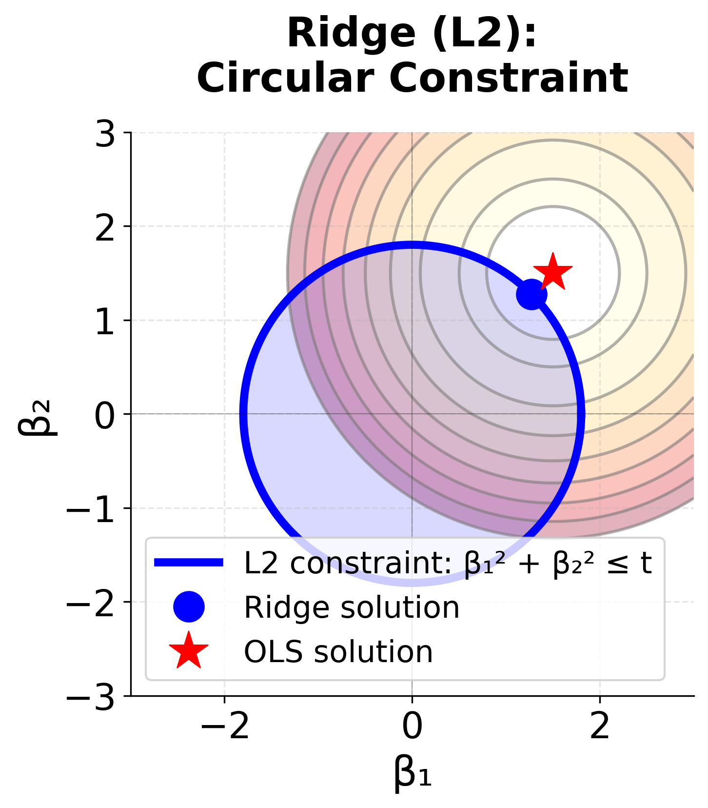
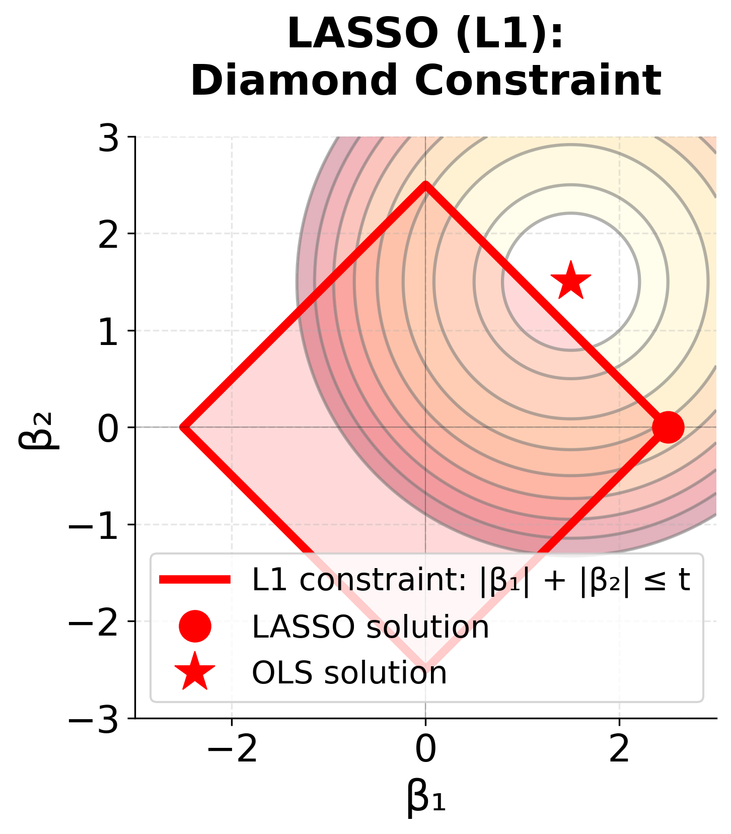
The geometric interpretation reveals why Ridge and LASSO behave differently. The contour lines (ellipses) represent the error surface—points closer to the red star (OLS solution) have lower error. The constraint regions (blue circle for Ridge, red diamond for LASSO) represent the penalty term. The optimal regularized solution occurs where the error contours first touch the constraint region.

For Ridge, the circular constraint has no corners, so the tangent point typically occurs away from the axes, meaning both β₁ and β₂ remain non-zero. For LASSO, the diamond has sharp corners on the axes, making it much more likely that the error contours will first touch the constraint at a corner, resulting in one coefficient being exactly zero (sparse solution).

Despite its advantages, Ridge regression has some limitations. Unlike LASSO, Ridge does not perform automatic feature selection since it does not drive coefficients exactly to zero, meaning all features remain in the final model. This can make the model less interpretable when dealing with datasets containing many irrelevant features. Additionally, Ridge requires careful tuning of the regularization parameter λ, and the optimal value may not be obvious without cross-validation. The method also assumes that all features are equally important for regularization, which may not be appropriate for datasets where some features are known to be more relevant than others.

The Ridge regression objective function is:

where:

• $\text{SSE}$ = sum of squared errors (measures how well the model fits the data)
• $\lambda$ = regularization parameter (controls the strength of the penalty; larger $\lambda$ means stronger regularization)
• $\beta_j$ = coefficient for feature $j$ (the parameter we're trying to estimate)
• $p$ = number of features (excluding the intercept $\beta_0$)
• $\sum_{j=1}^p \beta_j^2$ = L2 penalty term (sum of squared coefficients)

As for LASSO, we can write the Ridge regression objective function as a summation:

where:

• $y_i$ = actual (observed) value for observation $i$
• $\hat{y}_i = \beta_0 + \beta_1 x_{i1} + \beta_2 x_{i2} + \cdots + \beta_p x_{ip}$ = predicted value for observation $i$
• $\lambda$ = regularization parameter (non-negative; $\lambda \geq 0$)
• $\beta_0$ = intercept term (not penalized in Ridge regression)
• $\beta_j$ = coefficient for feature $j$ (where $j = 1, 2, \ldots, p$)
• $x_{ij}$ = value of feature $j$ for observation $i$
• $n$ = number of observations (sample size)
• $p$ = number of features (predictors)

This notation should look familiar from the previous section on LASSO. Rather than the L1 penalty, we have the L2 penalty, which is the sum of the squared coefficients.

This is the squared L2 norm (also called the L2 norm squared) of the coefficient vector $\boldsymbol{\beta}$, where $\|\boldsymbol{\beta}\|_2 = \sqrt{\sum_{j=1}^p \beta_j^2}$ is the L2 norm itself.

However, because matrix computations are much faster than summation, we can also write the Ridge regression objective function in matrix notation:

where:

• $\mathbf{y}$ = $n \times 1$ vector of target values (observed responses)
• $\mathbf{X}$ = $n \times p$ design matrix of features (each row is an observation, each column is a feature)
• $\boldsymbol{\beta}$ = $p \times 1$ vector of coefficients (parameters to estimate)
• $||\cdot||_2$ = L2 norm (Euclidean norm), defined as $||\mathbf{v}||_2 = \sqrt{\sum_i v_i^2}$
• $||\cdot||_2^2$ = squared L2 norm, defined as $||\mathbf{v}||_2^2 = \sum_i v_i^2$

Because we are not encountering issues of non-differentiability, we can find the closed-form solution for the Ridge regression objective function. Taking the derivative with respect to $\boldsymbol{\beta}$ and setting it to zero:

This yields the Ridge estimator:

where:

• $\hat{\boldsymbol{\beta}}_{Ridge}$ = Ridge regression coefficient estimates
• $\mathbf{X}^T$ = transpose of the design matrix
• $\mathbf{X}^T\mathbf{X}$ = $p \times p$ matrix (sum of squares and cross-products of features)
• $\lambda$ = regularization parameter
• $\mathbf{I}$ = $p \times p$ identity matrix (diagonal matrix with 1s on the diagonal and 0s elsewhere)
• $(\cdot)^{-1}$ = matrix inverse operation

• Bias-Variance Tradeoff: As $\lambda$ increases, bias increases but variance decreases
• Shrinkage: All coefficients are shrunk toward zero. In the special case of orthonormal features (where $\mathbf{X}^T\mathbf{X} = \mathbf{I}$), each coefficient is multiplied by the shrinkage factor $\frac{1}{1+\lambda}$, meaning $\hat{\beta}_{Ridge} = \frac{1}{1+\lambda}\hat{\beta}_{OLS}$
• Stability: The term $\lambda \mathbf{I}$ ensures $(\mathbf{X}^T\mathbf{X} + \lambda \mathbf{I})$ is always invertible, even when $\mathbf{X}^T\mathbf{X}$ is singular (non-invertible)
• Regularization Path: As $\lambda \to 0$, Ridge approaches OLS ($\hat{\boldsymbol{\beta}}_{Ridge} \to \hat{\boldsymbol{\beta}}_{OLS}$); as $\lambda \to \infty$, all coefficients approach zero ($\hat{\boldsymbol{\beta}}_{Ridge} \to \mathbf{0}$)

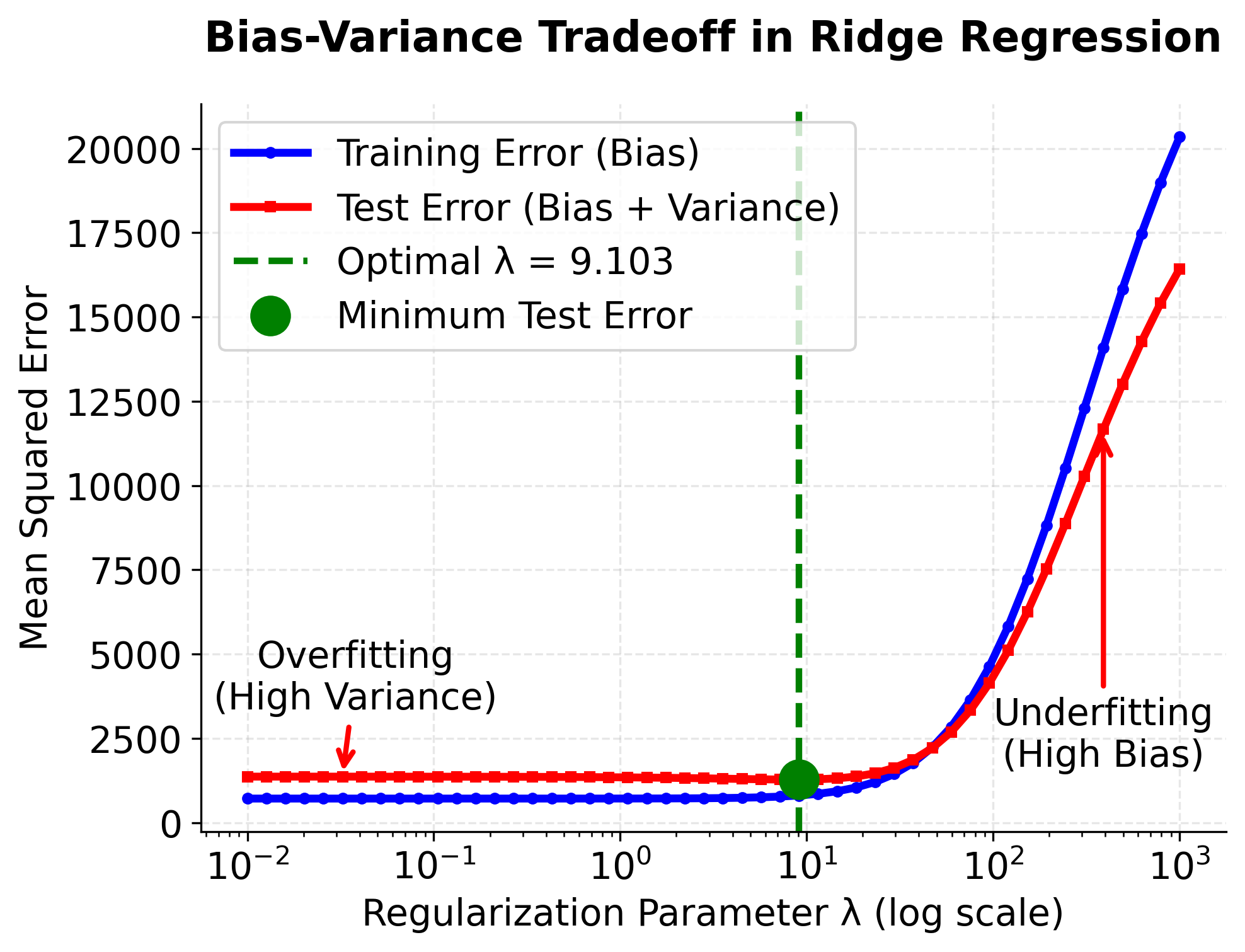
This visualization illustrates the fundamental bias-variance tradeoff in Ridge regression. When λ is very small (left side), the model is close to OLS and may overfit the training data, resulting in low training error but high test error due to high variance. As λ increases, the training error rises because the model becomes more constrained (increased bias), but the test error initially decreases as variance is reduced. The optimal λ (green line) achieves the best balance, minimizing test error. Beyond this point, further increasing λ causes underfitting, where the model becomes too simple and both training and test errors increase due to excessive bias.

We skipped over the derivation of the closed-form solution for Ridge regression, but it is similar to the derivation for LASSO, but easier since we are not encountering issues of non-differentiability, making the math more straightforward.

To better understand how Ridge regression affects multiple coefficients simultaneously, let's visualize the regularization path—how each coefficient changes as we increase λ.

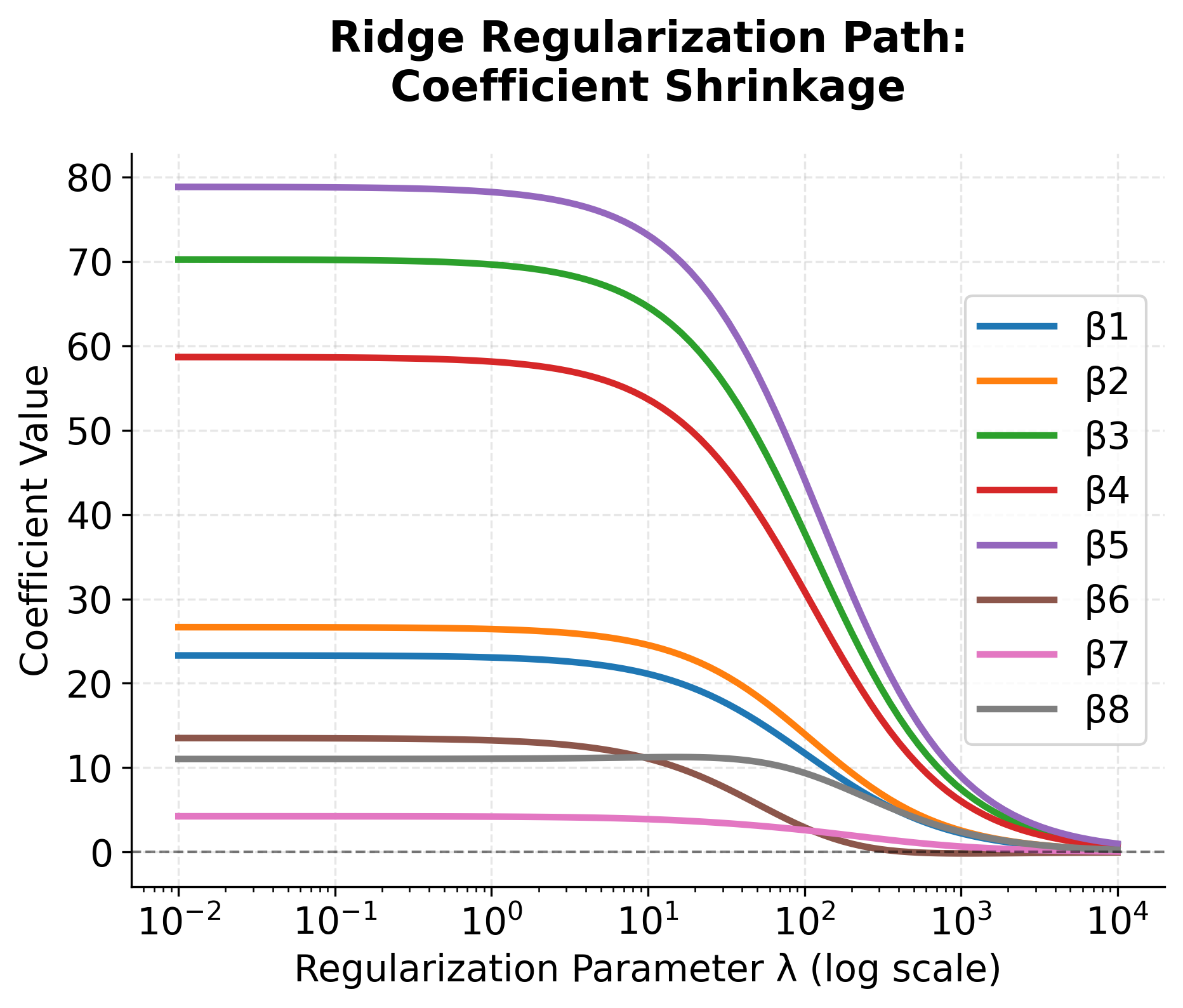
This plot reveals a key characteristic of Ridge regression: as λ increases, all coefficients shrink smoothly and continuously toward zero, but do not reach exactly zero. This is fundamentally different from LASSO, where coefficients can be driven to exactly zero. The smooth shrinkage means Ridge maintains all features in the model, which can be advantageous when all features are believed to be relevant or when dealing with highly correlated features.

Let's visualize Ridge regression by plotting the Ridge regression objective function for different values of $\lambda$.

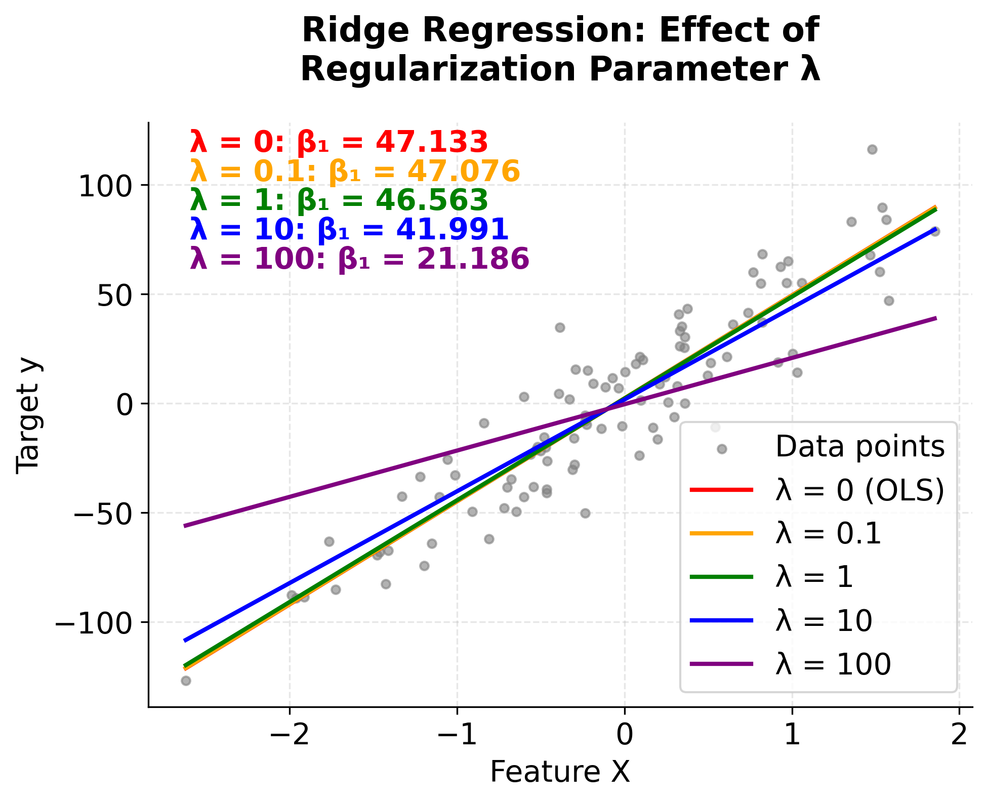
As we increase the regularization parameter λ from 0 to 100, we can see the regression line becoming flatter and the slope coefficient β₁ decreasing. When λ = 0 (red line), we get the standard OLS solution with the steepest slope. As λ increases, the penalty for large coefficients forces the model to use smaller coefficients, resulting in a more conservative fit that's less likely to overfit. The gray data points show the original dataset, and each colored line represents a different level of regularization. Notice how the coefficient values (shown in the text box) decrease as λ increases, demonstrating the shrinkage effect that is the hallmark of Ridge regression.

Let's work through a simple mathematical example to understand how Ridge regression works. We remind ourselves of the ridge estimator:

We'll use a small dataset with 3 observations and 2 features (excluding scaling to make the example easier to follow). Given following data:

• $n = 3$ observations
• $p = 2$ features
• $\lambda = 1$ (regularization parameter)

Let's walk through the Ridge regression calculation step by step.

Step 1: Calculate $\mathbf{X}^T\mathbf{X}$
First, we compute the matrix multiplication of the transpose of $\mathbf{X}$ and $\mathbf{X}$. This gives us the sum of squares and cross-products matrix of the features, which is used in both OLS and Ridge regression.

To verify: The $(1,1)$ element is $1^2 + 2^2 + 3^2 = 1 + 4 + 9 = 14$. The $(1,2)$ element is $1 \cdot 2 + 2 \cdot 3 + 3 \cdot 1 = 2 + 6 + 3 = 11$.

Note: This matrix is symmetric, meaning $X_{ij} = X_{ji}$ for all $i, j$. This is always true for $\mathbf{X}^T\mathbf{X}$.

Step 2: Add regularization term $\lambda \mathbf{I}$
Next, we add the regularization term $\lambda \mathbf{I}$ to the matrix. This penalizes large coefficients and helps prevent overfitting by making the matrix more stable. The resulting matrix is better conditioned, a term from numerical linear algebra that means small changes in input tend to produce small changes in output.

Step 3: Calculate $\mathbf{X}^T\mathbf{y}$
We then compute the product of the transpose of $\mathbf{X}$ and the target vector $\mathbf{y}$. This operation measures how each feature in $\mathbf{X}$ is correlated with the target variable $\mathbf{y}$. It forms the right-hand side of the normal equations used in both OLS and Ridge regression.

To verify: The first element is $1 \cdot 5 + 2 \cdot 8 + 3 \cdot 6 = 5 + 16 + 18 = 39$. The second element is $2 \cdot 5 + 3 \cdot 8 + 1 \cdot 6 = 10 + 24 + 6 = 40$.

Step 4: Find the inverse and solve
Now, we invert the regularized matrix from Step 2. This step is crucial for solving the linear system and finding the coefficients.

Note: In mathematics, the inverse of a $2 \times 2$ matrix $\begin{bmatrix} a & b \\ c & d \end{bmatrix}$ is given by $\frac{1}{ad-bc} \begin{bmatrix} d & -b \\ -c & a \end{bmatrix}$, provided $ad-bc \neq 0$. For larger matrices, the process involves more advanced linear algebra techniques such as Gaussian elimination or using determinants and adjugates.

In practice, when working with code, you can invert matrices using libraries like NumPy. For example, in Python, you can use np.linalg.inv(matrix) to compute the inverse of a matrix. However, for solving systems like Ridge regression, it's often more numerically stable to use np.linalg.solve() or specialized solvers rather than explicitly computing the inverse.

np.linalg.inv(A) explicitly computes the inverse of a matrix and then multiplies it by $b$, which is slower and can amplify numerical errors. In contrast, np.linalg.solve(A, b) directly solves the system $A x = b$ using efficient factorizations without forming the inverse, making it both faster and more numerically stable.

Step 5: Calculate Ridge coefficients
Finally, we multiply the inverse matrix by $\mathbf{X}^T\mathbf{y}$ to obtain the Ridge regression coefficients. These coefficients are shrunk compared to the OLS solution due to the regularization.

To verify the matrix multiplication:

• First element: $15 \cdot 39 + (-11) \cdot 40 = 585 - 440 = 145$
• Second element: $(-11) \cdot 39 + 15 \cdot 40 = -429 + 600 = 171$

Then dividing by 104: $145/104 \approx 1.394$ and $171/104 \approx 1.644$.

If we compare it with OLS which has no regularization ($\lambda = 0$), the OLS solution would be:

Let's calculate this step by step:

First, compute the determinant: $14 \cdot 14 - 11 \cdot 11 = 196 - 121 = 75$

Then multiply by $\mathbf{X}^T\mathbf{y}$:

where $14 \cdot 39 - 11 \cdot 40 = 546 - 440 = 106$ and $-11 \cdot 39 + 14 \cdot 40 = -429 + 560 = 131$.

Comparison:

• Ridge coefficients: $\begin{bmatrix} 1.394 \\ 1.644 \end{bmatrix}$
• OLS coefficients: $\begin{bmatrix} 1.413 \\ 1.747 \end{bmatrix}$

Notice how Ridge shrunk both coefficients toward zero compared to OLS, demonstrating the regularization effect. The first coefficient decreased from 1.413 to 1.394, and the second from 1.747 to 1.644.

Let's walk through a complete example of Ridge regression using scikit-learn. We'll demonstrate proper feature scaling, hyperparameter selection through cross-validation, and model evaluation.

First, we'll create a synthetic dataset and split it into training and test sets:

We've created a dataset with 1,000 samples and 10 features, splitting it 80/20 for training and testing. This gives us enough data to reliably evaluate the model's performance on unseen data.

Ridge regression's performance depends heavily on the regularization parameter α (lambda). We'll use cross-validation to find the best value:

The cross-validation results show how different regularization strengths affect model performance. The optimal α balances fitting the training data with preventing overfitting. Values that are too small (like 0.001) provide minimal regularization and may overfit, while values that are too large (like 100.0) over-regularize and underfit. Our cross-validation identified the sweet spot that minimizes prediction error on held-out data.

Now we'll train the final model using the optimal α and evaluate its performance on the test set:

The R² score indicates that our Ridge model explains approximately 99% of the variance in the target variable, demonstrating excellent predictive performance. The RMSE of around 50 represents the typical prediction error, which is reasonable given the noise level we introduced (50.0) when generating the data. This shows that Ridge regression successfully learned the underlying patterns while avoiding overfitting.

Let's look at the learned coefficients to understand how Ridge regularization affected them:

The coefficients show how each feature contributes to the prediction. Ridge regularization has shrunk these coefficients compared to what ordinary least squares would produce, helping prevent overfitting. None of the coefficients are exactly zero (unlike LASSO), which means all features remain in the model. The magnitude of each coefficient reflects both the feature's importance and the effect of regularization.

To see the effect of regularization, let's compare Ridge with unregularized OLS (α = 0):

The comparison reveals Ridge's regularization effect. While both models achieve similar R² scores on this dataset, Ridge's coefficients are smaller in magnitude than OLS coefficients, demonstrating the shrinkage effect. This shrinkage helps Ridge generalize better to new data, especially when dealing with multicollinearity or when the number of features is large relative to the number of observations. In practice, Ridge often provides more stable predictions than OLS, particularly on datasets with correlated features.

Below are the main parameters that control how Ridge regression works and performs.

• alpha: Regularization strength (λ in the mathematical formulation). Must be a positive float. Larger values specify stronger regularization, shrinking coefficients more toward zero. Default is 1.0. Use cross-validation to find the optimal value for your dataset.

• fit_intercept: Whether to calculate the intercept term (default: True). When True, the model learns a bias term β₀. When False, the model is forced to pass through the origin. Generally, keep this as True unless you have a specific reason to exclude the intercept.

• solver: Algorithm to use for optimization (default: 'auto'). Options include 'auto', 'svd', 'cholesky', 'lsqr', 'sparse_cg', 'sag', and 'saga'. The 'auto' option automatically selects the best solver based on the data type. For most cases, the default works well.

• max_iter: Maximum number of iterations for iterative solvers (default: None). Only used for 'sparse_cg', 'lsqr', 'sag', and 'saga' solvers. Increase if the solver doesn't converge.

• tol: Tolerance for stopping criteria (default: 1e-4). Smaller values mean more precise solutions but longer computation time. The default is usually sufficient.

• random_state: Seed for reproducibility when using stochastic solvers like 'sag' or 'saga' (default: None). Set to an integer to ensure consistent results across runs.

The following are the most commonly used methods for working with Ridge regression models.

• fit(X, y): Trains the Ridge regression model on the training data X and target values y. Returns the fitted model.

• predict(X): Returns predicted values for input data X using the trained model.

• score(X, y): Returns the R² score (coefficient of determination) on the given test data. Values closer to 1.0 indicate better fit.

• get_params(): Returns the model's hyperparameters as a dictionary. Useful for inspecting or saving model configuration.

• set_params(**params): Sets the model's hyperparameters. Useful for updating parameters without creating a new model instance.

Ridge regression is particularly valuable in scenarios where multicollinearity is present or when the number of features is large relative to the number of observations. In financial modeling and risk assessment, Ridge excels because financial variables are often highly correlated (such as different market indices or economic indicators), and Ridge provides stable coefficient estimates despite these correlations. The method is also highly effective when all features are believed to be relevant to the outcome, as Ridge maintains all features in the model rather than eliminating them.

The algorithm is especially useful in predictive modeling applications where generalization performance is more important than feature selection. Since Ridge shrinks coefficients smoothly without driving them to zero, it often provides better predictive accuracy than LASSO when most features contribute to the outcome. This makes it particularly valuable in domains like genomics, where thousands of genes may each have small effects on a phenotype, or in marketing analytics, where multiple customer attributes collectively influence behavior.

In high-dimensional settings where the number of features approaches or exceeds the number of observations, Ridge regression provides a stable solution where ordinary least squares would fail. The regularization term ensures that the matrix inversion remains numerically stable, making Ridge a reliable choice for problems with many correlated predictors. This stability is crucial in applications like image processing, text analysis, and sensor data modeling where feature dimensionality is naturally high.

The regularization parameter α (lambda) should be selected through cross-validation rather than arbitrary choice. Test a range of values on a logarithmic scale (such as 0.001, 0.01, 0.1, 1.0, 10.0, 100.0) and select the value that minimizes cross-validation error. For most datasets, the optimal α falls between 0.1 and 10.0, but this varies significantly depending on your data. Use at least 5-fold cross-validation to ensure robust parameter selection, and consider using RidgeCV from scikit-learn for efficient automated tuning.

When evaluating Ridge regression performance, use multiple metrics rather than relying on a single measure. The R² score indicates overall fit quality, while mean squared error and mean absolute error provide complementary information about prediction accuracy. Compare Ridge performance against both ordinary least squares (to assess the benefit of regularization) and LASSO (to determine whether feature selection would be beneficial). If Ridge and OLS perform similarly, your data may not require regularization, while large performance differences suggest that regularization is preventing overfitting.

Apply scaling within a pipeline to prevent data leakage between training and test sets. This ensures that scaling parameters (mean and standard deviation for StandardScaler, or min and max for MinMaxScaler) are computed only on training data and then applied to test data.

Ridge regression requires continuous target variables and works with both continuous and properly encoded categorical features. The method assumes linear relationships between features and the target, so examine your data for non-linear patterns before modeling. If non-linear relationships are present, consider polynomial feature expansion or interaction terms, though be aware that this increases dimensionality and may require stronger regularization.

Missing values must be handled before applying Ridge regression, as the algorithm cannot process incomplete observations. Use imputation strategies appropriate for your data type and missingness pattern. For numerical features, mean or median imputation often works well, while for categorical features, mode imputation or creating a separate "missing" category may be more appropriate. Outliers can influence Ridge estimates, though less severely than ordinary least squares due to the regularization penalty. Consider robust outlier detection methods and decide whether to remove, transform, or retain outliers based on domain knowledge.

Categorical variables require proper encoding before use with Ridge regression. Use one-hot encoding for nominal variables, which creates binary indicators for each category. For ordinal variables with meaningful order, label encoding may be appropriate. Be cautious with high-cardinality categorical variables, as one-hot encoding can create many features and increase computational requirements. In such cases, consider target encoding, frequency encoding, or grouping rare categories together.

One frequent mistake is applying Ridge regression without standardizing features, which causes features with larger scales to be penalized more heavily than features with smaller scales. This leads to biased coefficient estimates where the regularization effect varies across features based on their measurement units rather than their actual importance.

Another common issue is selecting the regularization parameter α without proper cross-validation. Choosing α based on training set performance or using an arbitrary value can lead to poor generalization. Values that are too small provide insufficient regularization and may not prevent overfitting, while values that are too large over-regularize the model and underfit the data.

Failing to compare Ridge with alternative methods can result in suboptimal model selection. While Ridge is effective for many problems, LASSO may be preferable when feature selection is desired, and elastic net (which combines L1 and L2 penalties) may perform better when you want both regularization and sparsity. Benchmark Ridge against these alternatives to ensure you're using the most appropriate method for your specific problem. Additionally, while Ridge maintains all features, the shrunken coefficients may be harder to interpret than unregularized estimates, especially when explaining models to non-technical stakeholders.

Ridge regression has O(np²) computational complexity for the closed-form solution, where n is the number of observations and p is the number of features. This makes it very efficient for most practical applications, typically completing in milliseconds for datasets with thousands of observations and hundreds of features. The closed-form solution is generally faster than iterative optimization methods used by LASSO, making Ridge a good choice when computational efficiency is important.

For large datasets (typically >100,000 observations) or high-dimensional data (p > 1,000), memory requirements can become substantial due to the need to compute and store the X^T X matrix. In such cases, consider using iterative solvers like stochastic gradient descent, which process data in batches and have lower memory requirements. The solver parameter in scikit-learn's Ridge implementation offers several options, with 'auto' automatically selecting the most appropriate solver based on your data characteristics.

When dealing with very high-dimensional data where p approaches or exceeds n, Ridge regression remains stable and computationally feasible, unlike ordinary least squares which becomes numerically unstable. The regularization term ensures that the matrix inversion is well-conditioned, making Ridge a reliable choice for high-dimensional problems. However, for extremely large feature spaces (p > 10,000), consider dimensionality reduction techniques like principal component analysis before applying Ridge to reduce computational requirements while maintaining predictive performance.

Ridge regression performance is typically evaluated using R², adjusted R², mean squared error (MSE), and root mean squared error (RMSE). Good performance indicators include R² values above 0.7 for most applications, though acceptable values vary significantly by domain. Cross-validation scores should be close to training scores to indicate good generalization—large differences suggest overfitting despite regularization, which may indicate that α is too small or that the linear assumption is violated.

When comparing Ridge to ordinary least squares, look for improvements in test set performance even if training performance is slightly worse. This indicates that regularization is successfully preventing overfitting. If Ridge and OLS perform similarly on test data, your problem may not require regularization, suggesting that the number of features is small relative to observations or that multicollinearity is not severe. Conversely, large performance improvements suggest that regularization is providing substantial value.

For deployment, Ridge regression's closed-form solution makes it highly scalable and suitable for real-time prediction systems. The linear nature of predictions allows for efficient computation even with large feature sets, and the model can be easily serialized and deployed across different platforms. However, the model requires that new data be scaled using the same parameters (mean and standard deviation) as the training data, so these scaling parameters must be saved and applied consistently in production. Monitor model performance over time, as the optimal α may change if the underlying data distribution shifts, requiring periodic retraining and hyperparameter tuning to maintain optimal performance.

Ridge regression (L2 regularization) is a technique that prevents overfitting by adding a penalty term proportional to the sum of squared coefficients. Unlike LASSO, Ridge shrinks coefficients toward zero but does not eliminate features entirely, making it well-suited for datasets with multicollinear features where all variables may be relevant. The method provides stable solutions even when the number of features exceeds the number of observations, and its closed-form solution makes it computationally efficient. However, Ridge requires careful feature scaling and parameter tuning to achieve optimal performance. It is particularly valuable in high-dimensional settings where maintaining all features while controlling overfitting is important.

Ready to test your understanding of Ridge regularization? Take this quiz to reinforce what you've learned about L2 regularization for regression.