

A comprehensive guide to Generalized Linear Models (GLMs), covering logistic regression, Poisson regression, and maximum likelihood estimation. Learn how to model binary outcomes, count data, and non-normal distributions with practical Python examples.

This article is part of the free-to-read Machine Learning from Scratch
Choose your expertise level to adjust how many terms are explained. Beginners see more tooltips, experts see fewer to maintain reading flow. Hover over underlined terms for instant definitions.
Generalized Linear Models (GLMs)
Generalized Linear Models (GLMs) are a flexible extension of ordinary linear regression that allows for modeling relationships between variables when the target variable doesn't follow a normal distribution or when the relationship isn't linear. In standard linear regression, we assume that the target variable is normally distributed and that the relationship between features and target is linear. However, many real-world problems involve different types of data—such as counts, binary outcomes, or categorical responses—that don't meet these assumptions.
GLMs address this by introducing two key components: a link function that connects the linear predictor to the expected value of the target, and an exponential family distribution that describes the probability distribution of the target variable. This framework allows us to model various types of data while maintaining the interpretability and computational efficiency of linear models.
In simple terms, GLMs are like a "smart adapter" that lets you use the power of linear regression even when your data doesn't follow the usual rules. Instead of forcing your data to fit a straight line, GLMs transform the data in clever ways so that linear regression techniques can still work effectively.
Models that you might have heard of that are GLMs are:
- Logistic Regression
- Poisson Regression
- Negative Binomial Regression
- Gamma Regression
- Inverse Gaussian Regression
- Tweedie Regression
- ...
Advantages
GLMs offer several key advantages over traditional linear regression. First, they provide a unified framework for modeling different types of response variables—binary, count, continuous, and categorical—without requiring entirely different methodologies. This makes GLMs particularly valuable when dealing with diverse datasets or when the nature of your target variable changes over time. GLMs also maintain the interpretability of linear models while being more flexible about the underlying data distribution. The link function provides a clear connection between the linear predictor and the expected response, making it easy to understand how changes in features affect the outcome. Additionally, GLMs are computationally efficient and have well-established statistical properties, including maximum likelihood estimation and hypothesis testing procedures.
Disadvantages
Despite their flexibility, GLMs have some limitations. The method assumes that the response variable follows a specific exponential family distribution, which may not always be appropriate for your data. If the chosen distribution doesn't match the true data generating process, the model may provide poor fits or misleading inferences. GLMs also assume that observations are independent, which can be problematic for time series data, clustered data, or other situations with dependencies. Additionally, while GLMs are more flexible than linear regression, they still assume a specific functional form through the link function, which may not capture complex nonlinear relationships present in the data. Finally, GLMs can be sensitive to outliers and may require careful model diagnostics to ensure assumptions are met.
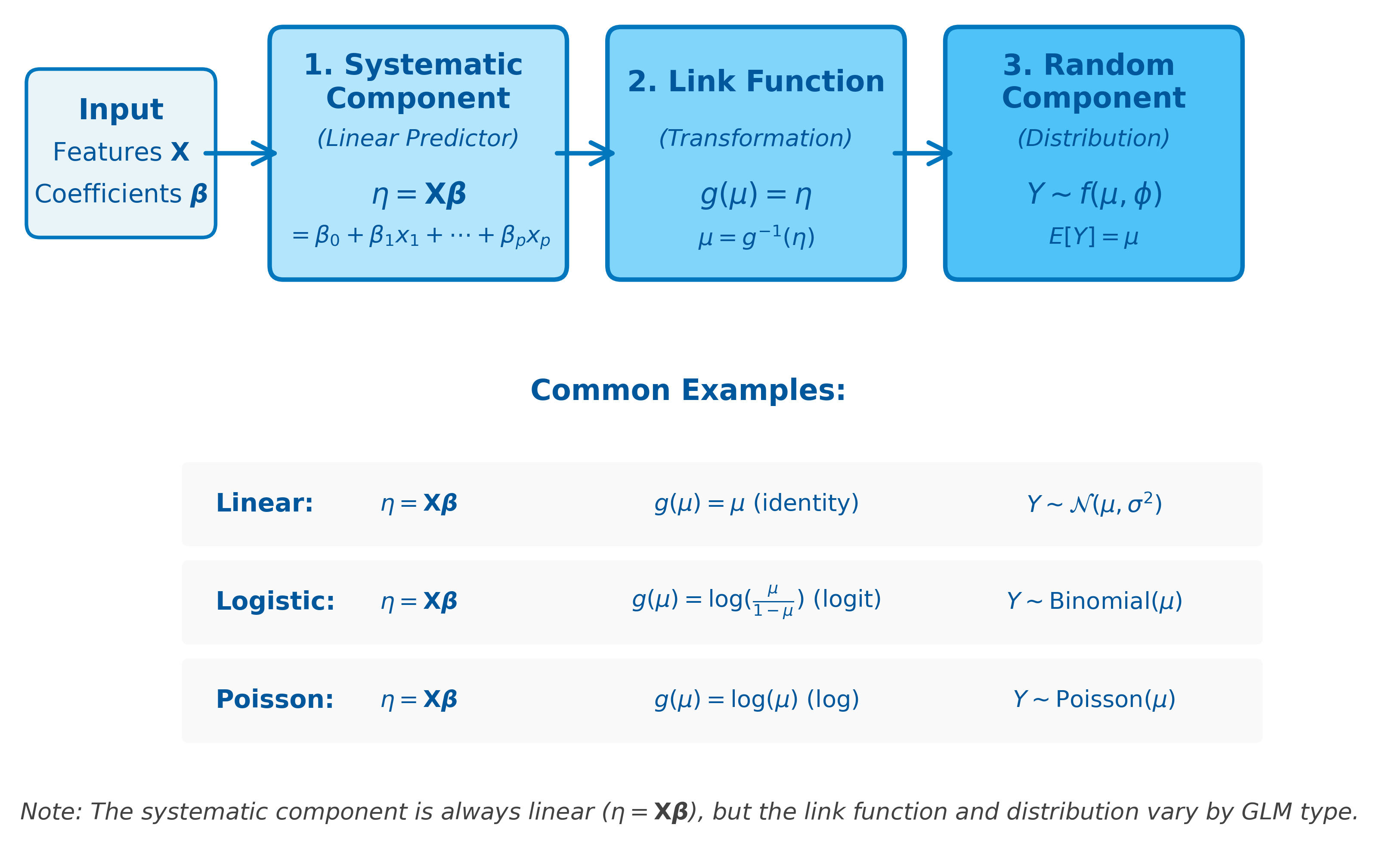
Components of GLMs
A Generalized Linear Model consists of three main components:
1. Random Component (Distribution)
The random component specifies the probability distribution of the response variable . GLMs assume that follows a distribution from the exponential family, which includes:
- Normal (Gaussian): For continuous data
- Binomial: For binary data (success/failure)
- Poisson: For count data
- Gamma: For positive continuous data
- Inverse Gaussian: For positive continuous data with specific variance properties
2. Systematic Component (Linear Predictor)
The systematic component is the linear combination of features:
where:
- is the linear predictor (a scalar value for a single observation, or a vector for multiple observations)
- is the intercept term (the expected response when all features equal zero)
- are the regression coefficients for each feature (quantify the effect of each feature on the linear predictor)
- are the feature values (predictor variables for a single observation)
- is the number of features (total count of predictor variables in the model)
This is identical to the linear predictor in ordinary linear regression.
3. Link Function
The link function connects the linear predictor to the expected value of the response :
where:
- is the link function (a monotonic, differentiable transformation that maps the mean response to the linear predictor scale)
- is the expected value (mean) of the response variable (the parameter we're modeling)
- is the linear predictor from the systematic component (the right-hand side of the equation: )
The link function transforms the expected response so that it can be modeled linearly. Different GLM families use different link functions appropriate for their response distributions.
Common GLM Types
Before diving into the specifics of each GLM type, it's important to understand that the choice of link function and probability distribution is what defines each model. The link function acts as a bridge between the linear predictor (the weighted sum of your features) and the expected value of the response variable. By selecting an appropriate link function and distribution, GLMs allow us to model a wide variety of data types using a unified framework.
In the following sections, we'll briefly introduce the most common GLM types—linear, logistic, and Poisson regression—to illustrate how the link function and model structure work together. Each of these models is covered in greater detail in its own dedicated chapter, where you'll find deeper mathematical explanations, practical examples, and implementation guidance. For now, consider this a high-level overview to set the stage for those more in-depth explorations.
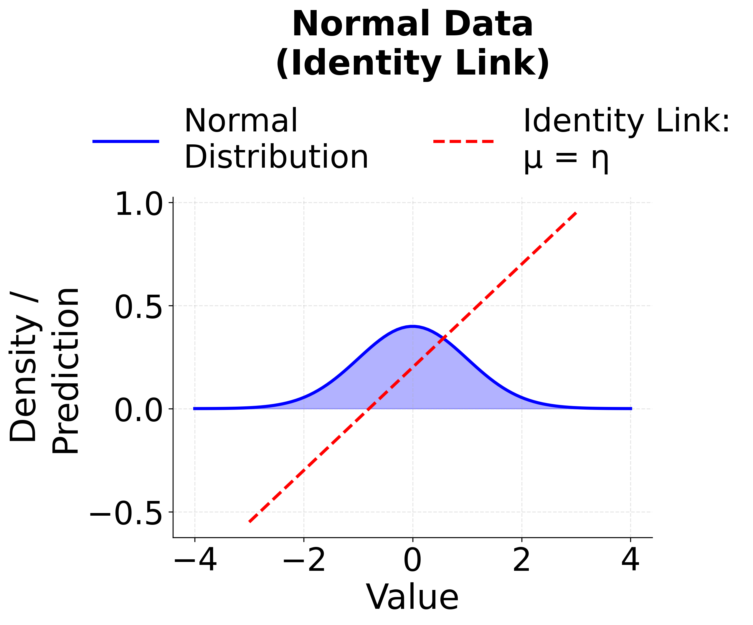
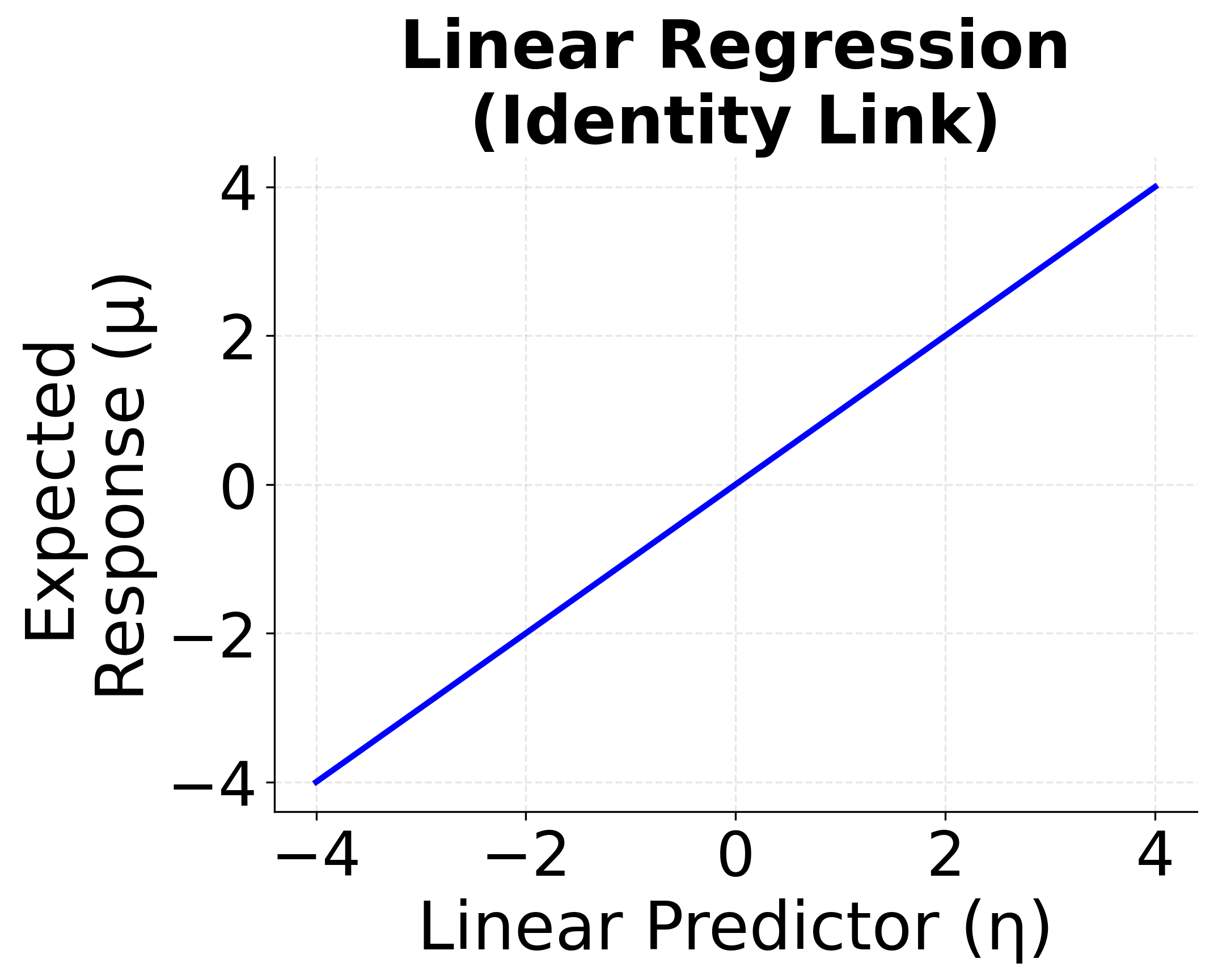
Linear Regression (Identity Link)
When the response variable is continuous and normally distributed, and the relationship between the predictors and the response is assumed to be linear, we use the identity link function. This is the classic linear regression model.
- Distribution: Normal (Gaussian)
- Link function: (identity)
- Model:
where:
- is the expected value of the response variable given the predictors (the conditional mean we're modeling)
- is the intercept (the expected response when all predictors equal zero)
- are the regression coefficients (quantify the linear effect of each predictor)
- are the predictor variables (the feature values)
- is the number of predictors
The identity link means that the expected response is modeled directly as a linear function of the features. This is the standard linear regression we've covered in previous sections, and it serves as the foundation for all GLMs.
When to use: Use linear regression when your outcome is continuous, unbounded, and approximately normally distributed. Examples include predicting house prices, heights, or temperatures.
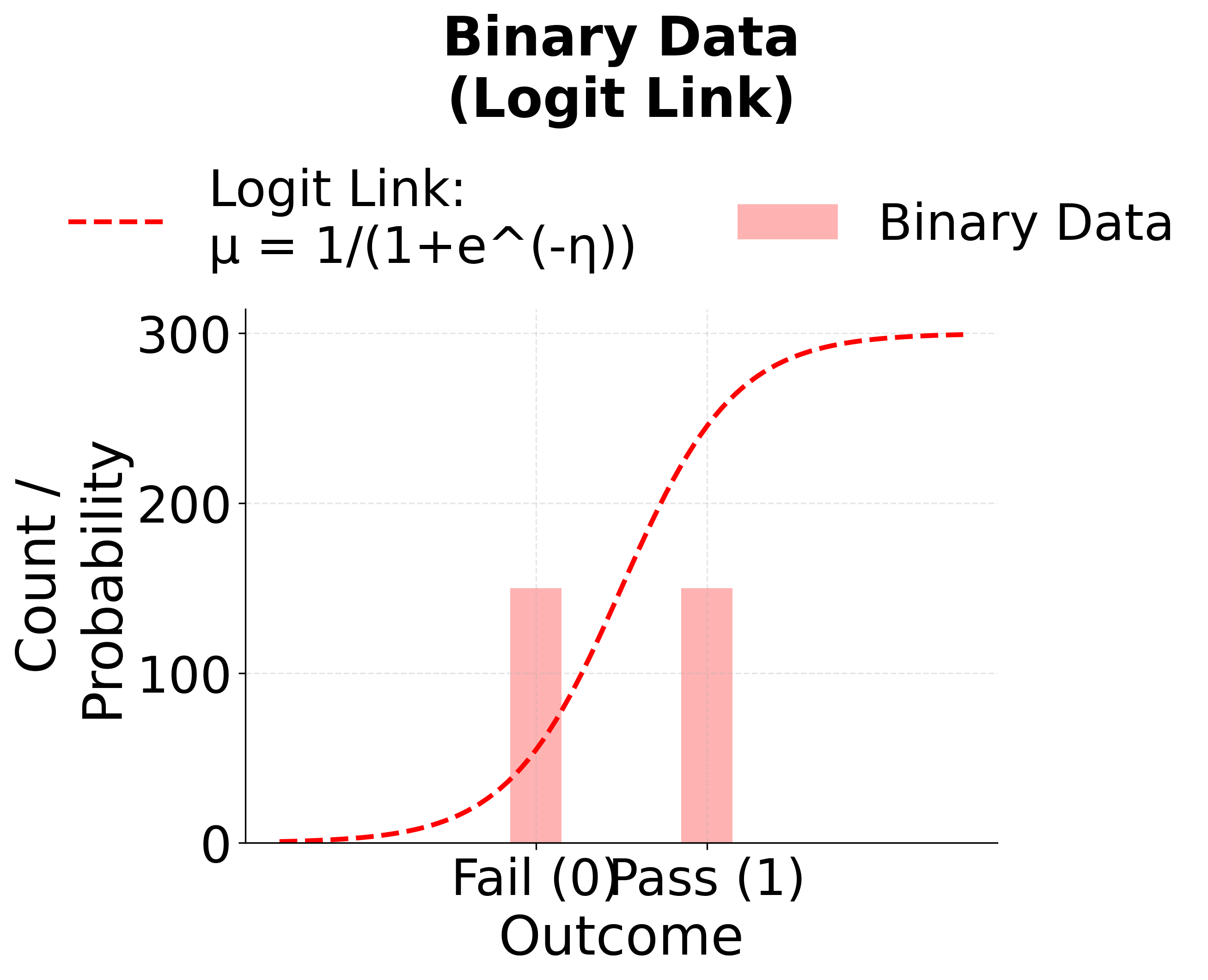
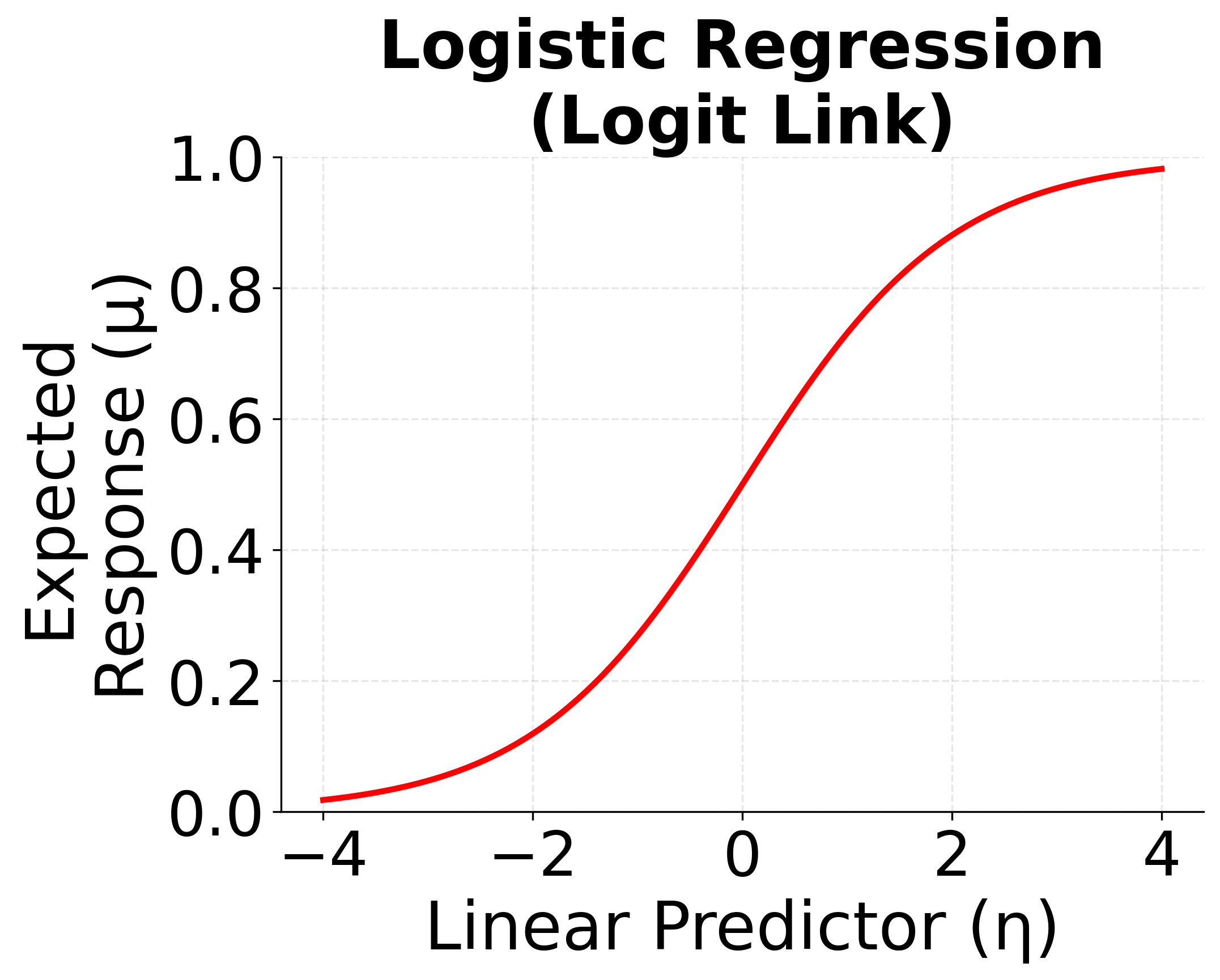
Logistic Regression (Logit Link)
When the response variable is binary (e.g., success/failure, yes/no, 0/1), logistic regression is the appropriate GLM. It uses the logit link function to model the probability of success.
- Distribution: Binomial
- Link function: (logit)
- Model:
where:
- is the probability that the response variable equals 1 (success) given predictors (the parameter we're modeling)
- is the odds of success (the ratio of the probability of success to the probability of failure)
- is the log-odds or logit (the natural logarithm of the odds)
- is the intercept (the log-odds when all predictors equal zero)
- are the regression coefficients (represent the change in log-odds for a one-unit increase in each predictor)
- are the predictor variables (the feature values)
The logit link transforms probabilities (which are constrained to be between 0 and 1) to the entire real line, allowing us to model them with a linear predictor.
When to use: Use logistic regression for binary classification tasks, such as predicting whether a customer will buy a product (yes/no), or whether an email is spam (spam/not spam).
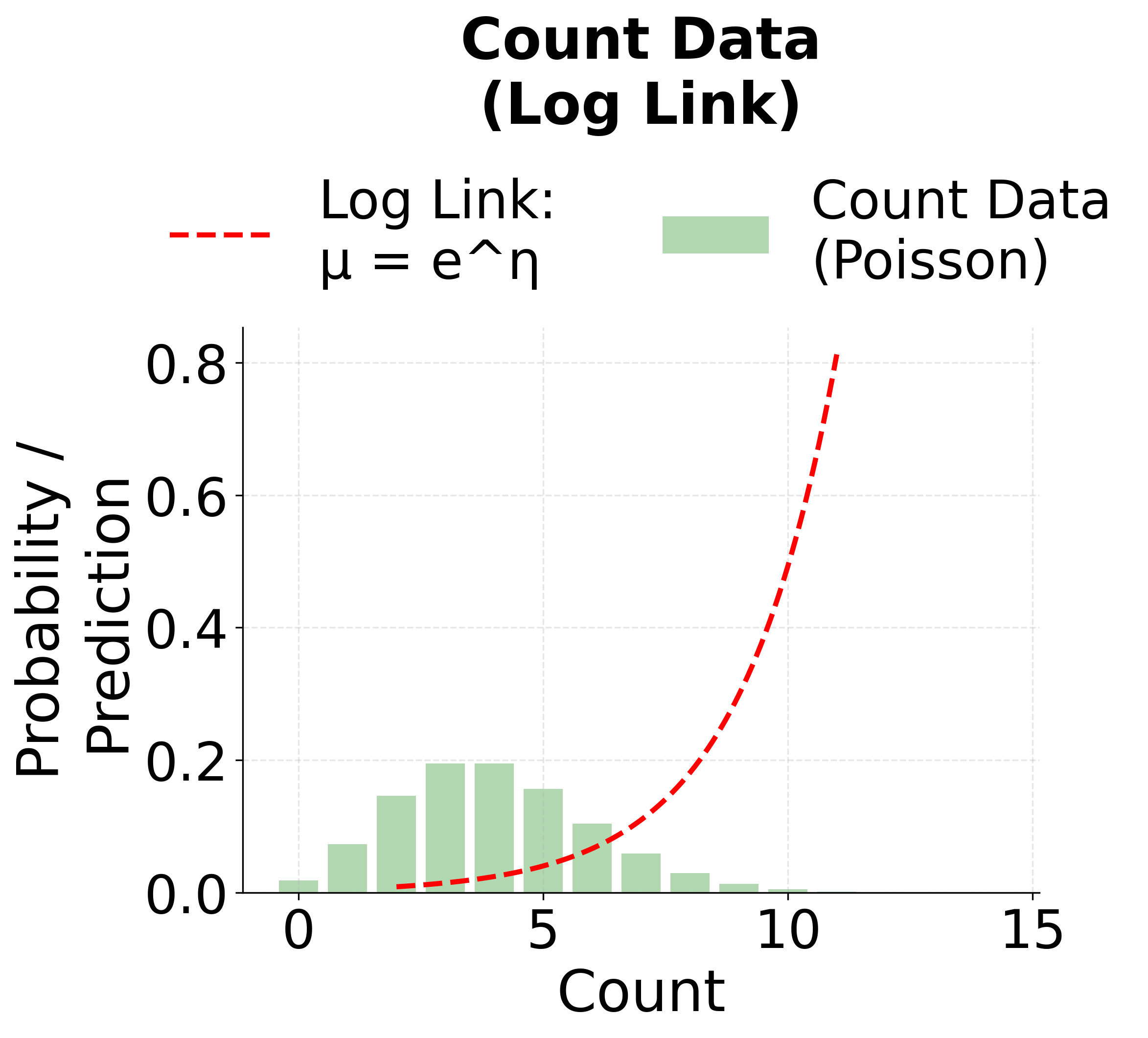
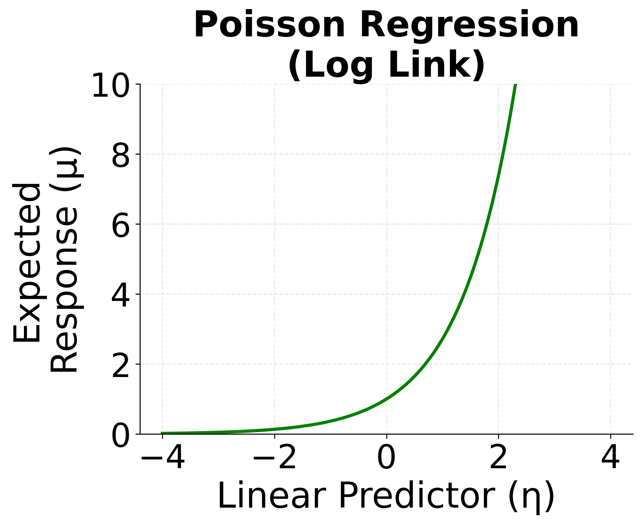
Poisson Regression (Log Link)
For modeling count data—where the response variable represents the number of times an event occurs—Poisson regression is used. It employs the log link function to ensure that the predicted counts are non-negative.
- Distribution: Poisson
- Link function: (log)
- Model:
where:
- is the expected count (mean of the Poisson distribution) given predictors (the rate parameter we're modeling)
- is the natural logarithm of the expected count (the link function applied to the mean)
- is the intercept (the log of the expected count when all predictors equal zero)
- are the regression coefficients (represent the change in log-count for a one-unit increase in each predictor)
- are the predictor variables (the feature values)
The log link ensures that the predicted mean is positive. By inverting the log link, we get:
where:
- is Euler's number (approximately 2.718)
- The exponential function is positive for any real value
- This ensures , which is necessary for count data (counts cannot be negative)
When to use: Use Poisson regression when your outcome is a count (e.g., number of customer visits, number of accidents, number of emails received in an hour), and the counts are non-negative integers.
These three models—linear, logistic, and Poisson regression—are the most common and foundational examples of GLMs. Each is defined by its choice of distribution and link function, allowing you to tailor the model to the nature of your response variable.
The models and link functions described above are all classic examples of Generalized Linear Models (GLMs). While this list is not exhaustive, these are among the most commonly used GLM types in practice. Rest assured, the model forms and link functions presented here are correct; we will explore the mathematical details and reasoning behind the most popular ones in the following sections.
Formula
The general GLM formula can be written as:
where:
- is the expected value of the response variable given the features (the conditional mean)
- is the link function (transforms the expected response to the linear predictor scale)
- is the intercept term
- are the regression coefficients (one for each feature)
- are the feature values (predictor variables)
- is the number of features
This reads as: "The link function applied to the expected value of the response equals the linear combination of features with their coefficients."
Matrix Notation
In matrix form, the GLM can be written as:
where:
- is the vector of expected responses (one element per observation, where and )
- is the design matrix of features (each row is one observation, each column is one feature, with the first column typically being all 1s for the intercept)
- is the vector of coefficients ()
- is applied element-wise to (producing a vector where each element is )
- is the number of observations
How GLM Components Work Together
The following diagram illustrates how the three components of a GLM connect to transform input features into predictions:
Maximum Likelihood Estimation
Unlike linear regression, GLMs typically don't have closed-form solutions and require iterative optimization to find the maximum likelihood estimates of the parameters. The likelihood function for a GLM is:
where:
- is the likelihood function (the probability of observing the data given the parameters)
- is the vector of regression coefficients ()
- is the number of observations in the dataset
- is the probability density function (for continuous responses) or probability mass function (for discrete responses) of the chosen distribution for observation
- is the observed response value for observation
- is the vector of predictor values for observation (i.e., where the first element is 1 for the intercept)
- denotes the product over all observations (reflecting the assumption of independent observations)
The log-likelihood is:
where:
- is the log-likelihood function (the logarithm of the likelihood)
- denotes the natural logarithm
- denotes the sum over all observations
- Taking the logarithm converts the product to a sum, which is computationally more stable and prevents numerical underflow when dealing with many small probabilities
The maximum likelihood estimates are found by solving:
where:
- is the maximum likelihood estimate of the coefficient vector (the value that makes the observed data most probable)
- finds the value of that maximizes the log-likelihood function
This is typically done using Iteratively Reweighted Least Squares (IRLS), which is an iterative algorithm that solves a sequence of weighted least squares problems.
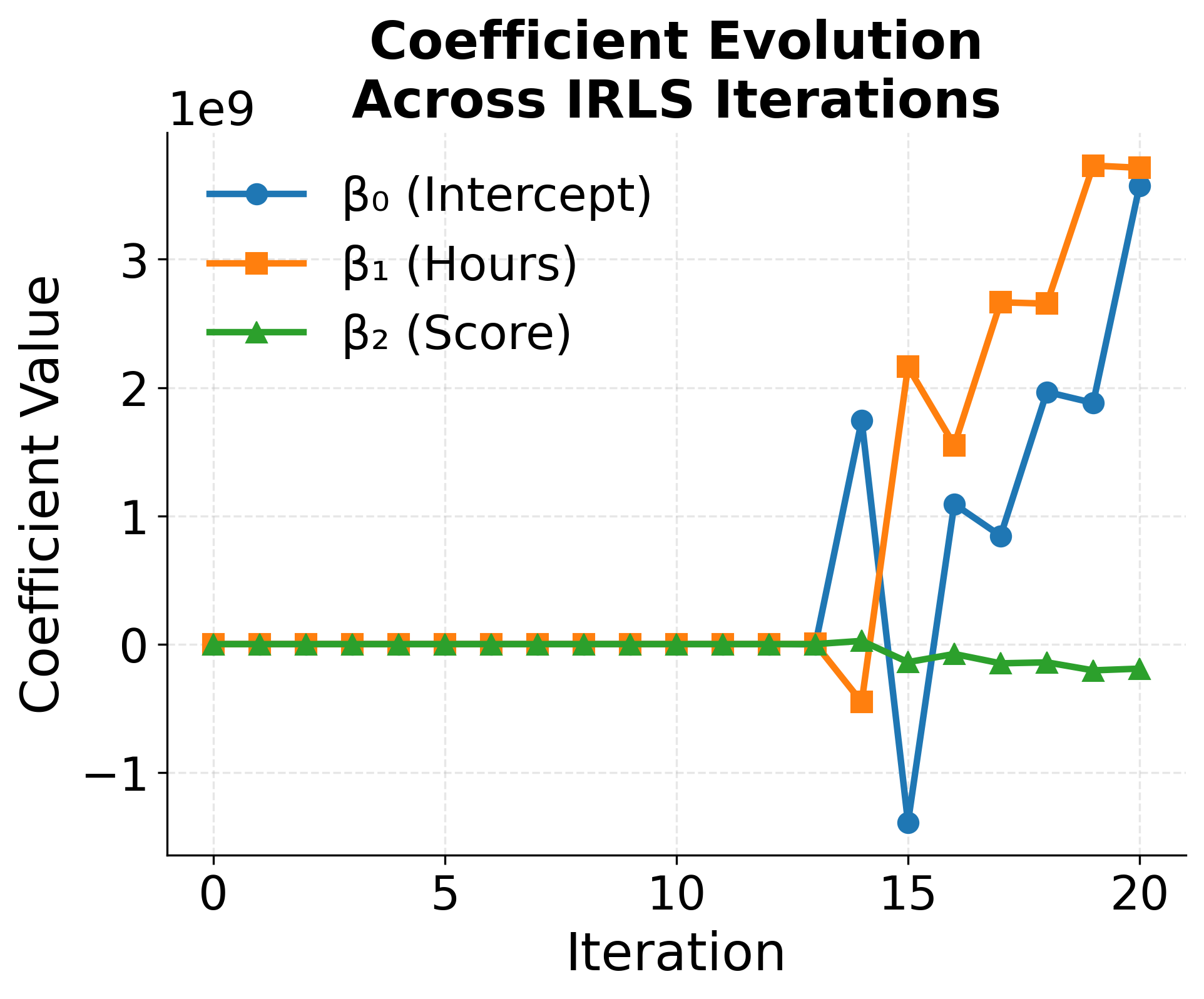
Example: Logistic Regression
Let's work through a detailed example of logistic regression, which is one of the most common GLMs. Suppose we want to predict whether a student will pass an exam based on their study hours and previous test scores.
Data:
- Study hours: [2, 3, 4, 5, 6, 7, 8]
- Previous scores: [60, 65, 70, 75, 80, 85, 90]
- Pass (1) or Fail (0): [0, 0, 1, 1, 1, 1, 1]
This is our model specification:
- Distribution: Binomial
- Link function: Logit
- Model:
Let's solve this step by step.
Step 1: Set up the design matrix
First, we organize our data into a matrix form suitable for regression. Each row of the matrix corresponds to one observation (student), and each column is a feature (including a column of 1s for the intercept). For our example, the features are:
- Intercept (always 1)
- Study hours
- Previous test score
So, for our 7 students, the design matrix looks like:
The corresponding response vector (whether the student passed) is:
Step 2: Initialize coefficients
We start the iterative process by choosing initial values for the coefficients (the parameters). A common choice is to set all coefficients to zero:
This means our initial model predicts the same probability for all students, regardless of their features.
Step 3: IRLS (Iteratively Reweighted Least Squares) Iteration
The IRLS algorithm updates the coefficients in a series of steps, using the current estimate to improve the next one. For each iteration :
Note: The following steps are a detailed explanation of the IRLS algorithm to demonstrate the process. We will not go into the very specific details of the algorithm in this section. In reality, you would not compute the IRLS algorithm by hand. Modern statistical and machine learning libraries (like NumPy, scikit-learn, R, and others) implement this algorithm efficiently.
-
Calculate the linear predictor:
Compute .where:
- is the vector of linear predictors at iteration (one entry per observation)
- is the design matrix (each row is one observation)
- is the coefficient vector at iteration
- For the first iteration with , all entries in equal 0
-
Calculate fitted values (predicted probabilities):
Apply the inverse link function (the logistic sigmoid for logistic regression) to get the predicted probability of passing for each student:where:
- is the vector of fitted values (predicted probabilities) at iteration
- is the inverse link function (for logistic regression, this is the logistic sigmoid function)
- The formula is applied element-wise: for each observation
- For the first iteration with , all predicted probabilities equal 0.5 (since )
-
Calculate the working response:
This step creates a "pseudo-response" that allows us to use weighted least squares:where:
- is the vector of working responses at iteration (adjusted target values for the weighted least squares step)
- is the vector of observed responses (actual outcomes: 0 or 1 for each observation)
- is the residual vector (difference between actual and predicted values)
- is computed element-wise and represents the variance of the Bernoulli distribution for each observation (i.e., )
- Division is performed element-wise
-
Calculate the weights:
The weights for each observation are based on the variance of the predicted probability:where:
- is an diagonal weight matrix at iteration
- creates a diagonal matrix with the elements of vector on the diagonal
- The diagonal entries are , which is the variance of the Bernoulli distribution for observation
- Observations with predicted probabilities near 0.5 receive higher weights (maximum variance of 0.25), while those near 0 or 1 receive lower weights
-
Update the coefficients:
Solve the weighted least squares problem to get the new coefficient estimates:where:
- is the updated coefficient vector for iteration
- is the transpose of the design matrix
- is the inverse of the weighted cross-product matrix (analogous to in ordinary least squares)
- This formula is the solution to the weighted least squares problem: minimize
Step 4: Check for convergence
After each iteration, check if the coefficients have stabilized:
where:
- is the Euclidean norm (also called the L2 norm), which measures the magnitude of a vector:
- is the coefficient vector at iteration (the newly updated coefficients)
- is the coefficient vector at iteration (the previous coefficients)
- is the change in coefficients between iterations
- is a small tolerance threshold (e.g., ), which defines how close to convergence we need to be
If the change is smaller than , the algorithm has converged. Otherwise, repeat the steps above with the new coefficients. The process continues until the change in coefficients is very small, indicating that we've found the maximum likelihood estimates.
Summary of what happens
- We start with all coefficients at zero (no effect from features).
- At each step, we use the current model to predict probabilities, then adjust the coefficients to better fit the observed outcomes, giving more weight to observations where the model is less certain.
- This process repeats, gradually improving the fit, until the coefficients stop changing significantly.
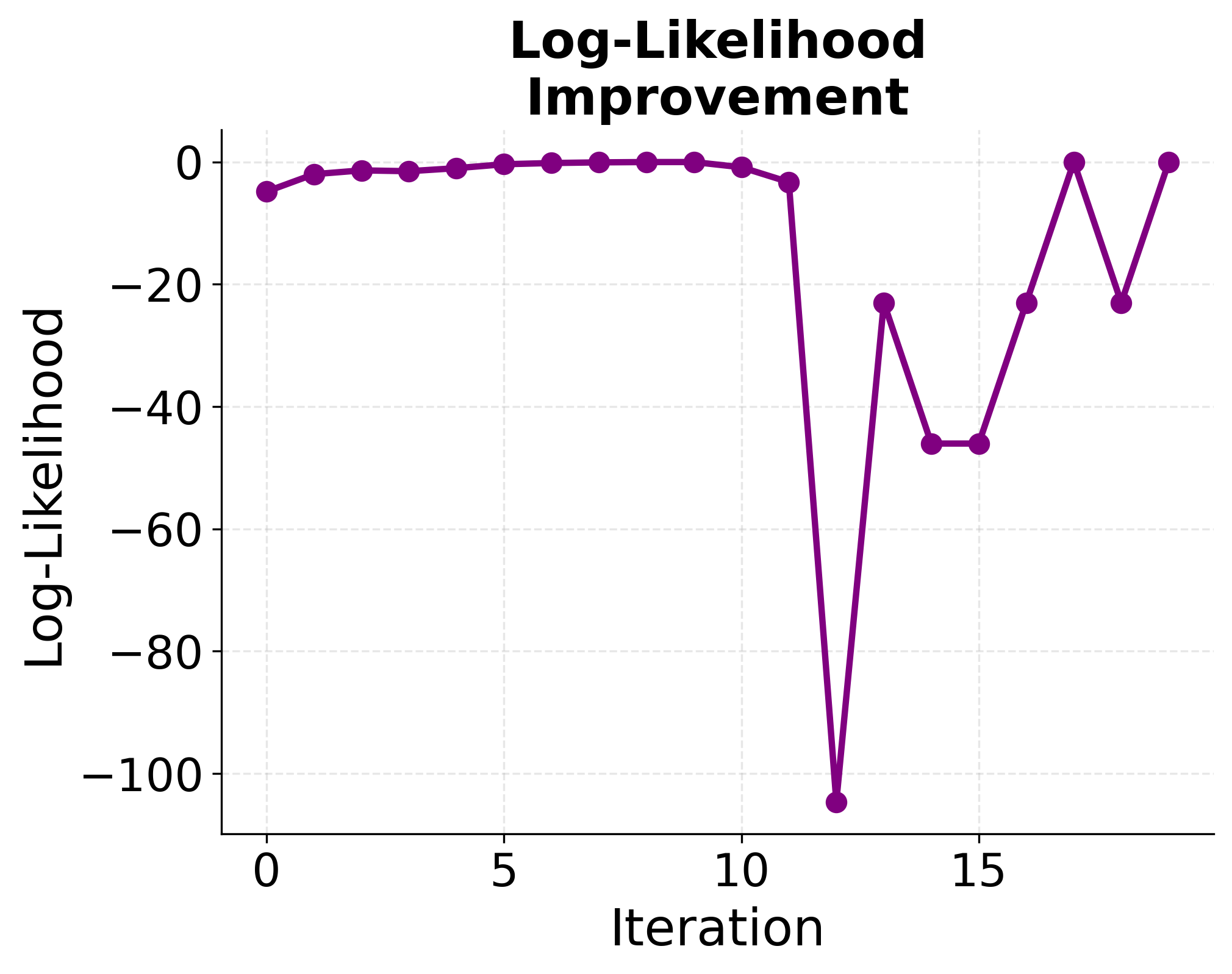
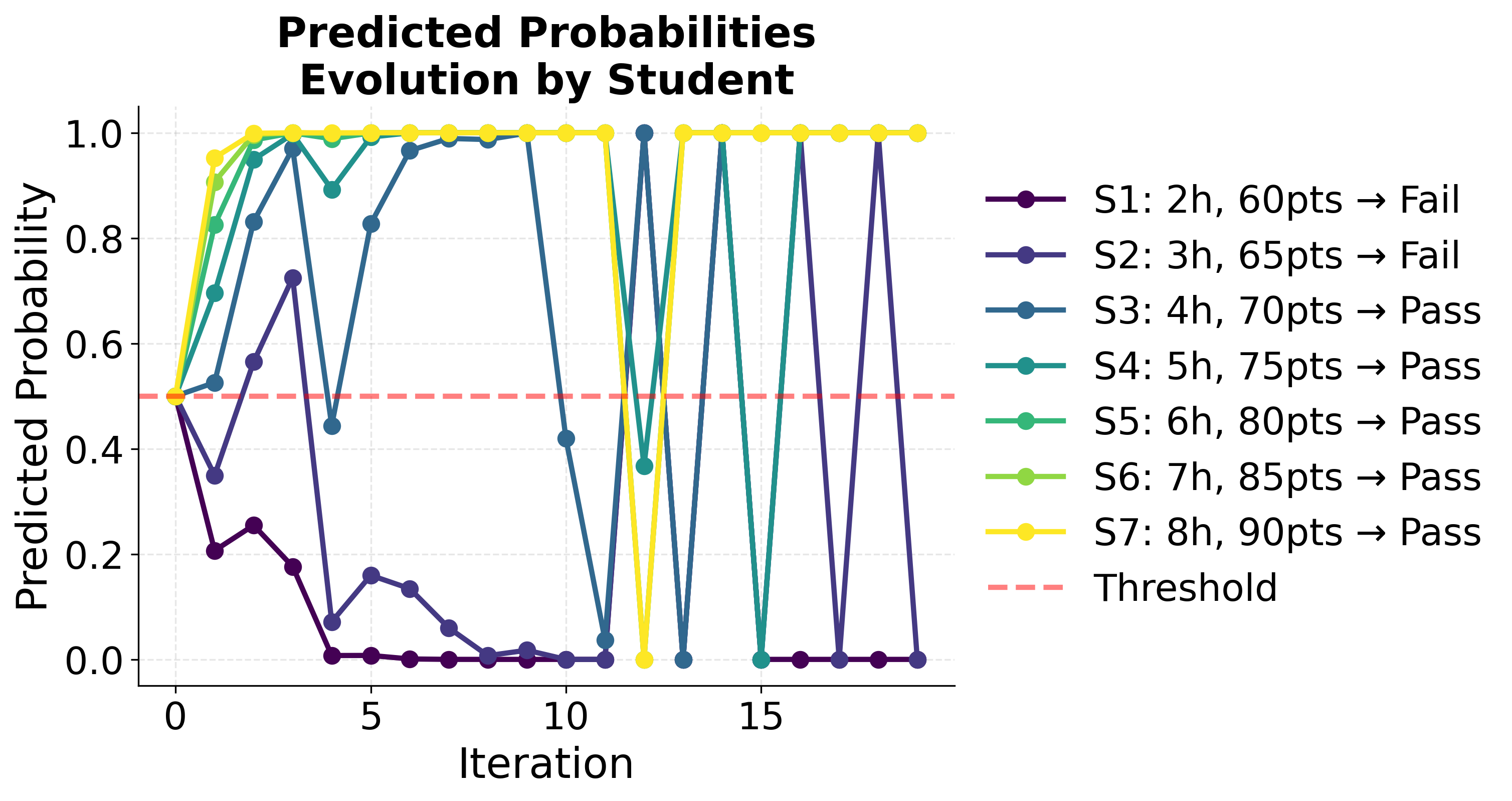
Final Results
After convergence (typically after 5-10 iterations), we obtain the maximum likelihood estimates:
where:
- is the estimated intercept
- is the estimated coefficient for study hours
- is the estimated coefficient for previous scores
So the fitted model is:
Interpretation
The coefficients in a logistic regression model represent the change in log-odds for a one-unit increase in the predictor variable, holding all other variables constant.
- For each additional hour of study, the log-odds of passing increase by 0.8
- For each additional point on previous scores, the log-odds of passing increase by 0.1
Example calculation: To find the probability of passing for a student with 5 hours of study and a previous score of 75, we substitute these values into the fitted model.
Step 1: Calculate the linear predictor (log-odds)
where:
- is the linear predictor (the log-odds of passing)
- is the intercept (baseline log-odds when all features are zero)
- is the contribution from study hours (each hour adds 0.8 to the log-odds)
- is the contribution from previous scores (each point adds 0.1 to the log-odds)
- The sum is the total log-odds for this student
Step 2: Convert log-odds to probability
Then, we apply the inverse logit function (logistic sigmoid) to convert log-odds to probability:
where:
- is the predicted probability of passing (the outcome we want)
- is the exponential of the negative linear predictor
- (computed using a calculator or computer)
- The denominator represents the normalization factor
- The final probability or 2.4%, indicating this student is very unlikely to pass
Interpretation: With only 5 hours of study and a previous score of 75, the model predicts a 2.4% chance of passing. This low probability suggests that either more study hours or a higher previous score (or both) would be needed for a reasonable chance of success.
One of the major advantages of GLMs is that, despite their flexibility, they retain many of the familiar tools and interpretability of linear regression. This means we can perform hypothesis testing, construct confidence intervals, and assess the significance and impact of each feature in the model—just as we do in ordinary linear regression. As a result, GLMs provide both statistical rigor and insight into how each predictor influences the outcome.
Visualizing GLMs
The following visualizations demonstrate how different link functions transform the linear predictor to produce the expected response. Each GLM type uses a specific link function that is mathematically appropriate for its target distribution. The identity link maintains linearity for continuous normal data, the logit link produces S-shaped probabilities for binary outcomes, and the log link ensures positive predictions for count data.
Implementation
In this section, we'll demonstrate how to implement Generalized Linear Models in Python using scikit-learn. We'll work through practical examples of logistic regression (for binary classification) and Poisson regression (for count data), showing how to train models, evaluate performance, and interpret results.
Logistic Regression for Binary Classification
Let's start with a logistic regression example using the breast cancer dataset. This demonstrates how to use a GLM with a binomial distribution and logit link for binary classification.
Data Preparation
We'll start by loading the breast cancer dataset and preparing it for modeling. This dataset contains features computed from digitized images of breast mass, and our goal is to predict whether a tumor is malignant or benign.
The dataset is split into 80% training and 20% testing data using stratified sampling to maintain the class distribution. Feature standardization transforms all variables to have zero mean and unit variance, which is crucial for logistic regression because it helps the optimization algorithm converge faster and produces more stable coefficient estimates. Without standardization, features with larger scales would dominate the model.
Model Training
Now we'll train a logistic regression model using L2 regularization (ridge penalty) with the L-BFGS solver, which is efficient for this dataset size:
Model Performance
Let's examine the model's performance on the test set:
With an accuracy above 95% and a ROC AUC score close to 1.0, the model demonstrates excellent performance in distinguishing between malignant and benign tumors. The ROC AUC score near 1.0 is particularly important—it indicates that the model can effectively rank predictions, placing malignant cases higher than benign ones across different probability thresholds. The convergence in a reasonable number of iterations confirms that the optimization process was stable and the model parameters are reliable.
The classification report reveals balanced performance across both tumor types. Precision values above 0.95 indicate that when the model predicts a tumor is malignant (or benign), it's correct more than 95% of the time. Similarly, recall values above 0.95 show that the model successfully identifies more than 95% of actual malignant (and benign) cases. The F1-scores, which balance precision and recall, exceed 0.95 for both classes, confirming that the model doesn't favor one class over the other—a crucial property for medical diagnosis applications.
The confusion matrix provides a clear picture of where the model succeeds and where it occasionally errs. The diagonal elements (true negatives and true positives) are substantially larger than the off-diagonal elements (false positives and false negatives), indicating that most predictions are correct. In medical contexts, false negatives (predicting benign when actually malignant) are particularly concerning because they could delay treatment. The very low count of false negatives demonstrates that the model is reliable for clinical screening purposes.
Coefficient Interpretation
Let's examine the most influential features:
Each coefficient represents how much the log-odds of malignancy change when that feature increases by one standard deviation (since we standardized the features). Positive coefficients push predictions toward malignancy, while negative coefficients push toward benign. The magnitude of each coefficient indicates its importance: features with larger absolute values exert stronger influence on the final prediction. For instance, if "worst concave points" has a large positive coefficient, it means that higher values of this feature strongly suggest malignancy.
Poisson Regression for Count Data
Now let's demonstrate Poisson regression, which is appropriate for modeling count data. We'll create a synthetic dataset representing the number of customer visits to a store based on various factors.
Data Generation
This synthetic dataset simulates a realistic scenario where customer visits follow a Poisson distribution—a natural choice for count data. We've embedded a known relationship between visits and three factors: advertising spend, temperature, and weekend status. The goal is to see if our Poisson regression model can recover these true relationships from the data, demonstrating how the method works in practice.
Model Training
Model Performance
The low MAE (Mean Absolute Error) and RMSE (Root Mean Squared Error) indicate that predictions are typically within a few visits of the actual counts—excellent performance for this type of problem. More importantly, the mean predicted visits closely match the mean actual visits, showing that the model has correctly learned both the overall scale and the relative patterns in the data. This suggests the model has successfully recovered the underlying Poisson process that generated the data.
Coefficient Analysis
In Poisson regression, coefficients represent the change in log-count for a one-unit increase in the predictor, holding all other variables constant. To interpret the practical effect:
- Coefficient (): The change in for a one-unit increase in the predictor
- Exponentiated coefficient (): The multiplicative effect on the expected count
- Percentage change: gives the percentage change in expected count
For example, if and , this means a one-unit increase in the predictor multiplies the expected count by 1.0202, which is a 2.02% increase. The weekend effect shows a substantial increase in expected visits, as designed in our data generation process.
Prediction Example
Let's make predictions for specific scenarios:
These scenario-based predictions illustrate how the model integrates multiple factors to produce realistic visit estimates. Comparing scenarios 1 and 2 (which differ only in weekend status) reveals the substantial weekend effect—visits increase significantly on weekends even with identical advertising and temperature. Similarly, comparing scenarios 1 and 3 shows how increased advertising spend and warmer temperature boost predicted visits. These patterns align perfectly with the coefficients we examined earlier, confirming that the model has learned interpretable and actionable relationships.
Key Parameters
Below are the main parameters that affect how GLMs work and perform in scikit-learn.
LogisticRegression Parameters
penalty: Type of regularization applied to prevent overfitting (default: 'l2'). Options include 'l1' (lasso), 'l2' (ridge), 'elasticnet', or 'none'. L2 regularization works well for most cases and is computationally efficient. L1 can perform feature selection by driving some coefficients to exactly zero.C: Inverse of regularization strength (default: 1.0). Smaller values (e.g., 0.01-0.1) apply stronger regularization and help prevent overfitting, while larger values (e.g., 10-100) reduce regularization. Start with 1.0 and adjust based on validation performance.solver: Optimization algorithm (default: 'lbfgs'). Options include 'lbfgs', 'liblinear', 'newton-cg', 'sag', and 'saga'. Use 'lbfgs' for most problems with L2 penalty, 'liblinear' for small datasets, and 'saga' for large datasets or when using L1/elasticnet penalties.max_iter: Maximum number of iterations for convergence (default: 100). Increase to 1000 or higher if you encounter convergence warnings. More iterations allow the optimizer more time to find the optimal solution.class_weight: Weights assigned to each class (default: None). Set to 'balanced' for imbalanced datasets to automatically adjust weights inversely proportional to class frequencies. This helps the model pay more attention to minority classes.random_state: Random seed for reproducibility (default: None). Set to an integer (e.g., 42) when using solvers with randomness ('sag', 'saga') to ensure consistent results across runs.
PoissonRegressor Parameters
alpha: L2 regularization strength (default: 1.0). Controls the penalty on coefficient magnitudes. Smaller values (0.01-0.1) reduce regularization for complex patterns, while larger values (10-100) increase regularization to prevent overfitting. Start with 1.0 and tune based on validation performance.max_iter: Maximum number of iterations (default: 100). Increase if the model doesn't converge within the default limit. Convergence warnings indicate the optimizer needs more iterations to find the optimal solution.tol: Convergence tolerance (default: 1e-4). The optimization stops when the change in parameters falls below this threshold. Smaller values (e.g., 1e-6) require more precise convergence but take longer to train.warm_start: Whether to reuse the previous solution as initialization (default: False). Set to True when fitting multiple times with different parameters (e.g., during hyperparameter tuning) to speed up convergence.
Key Methods
The following are the most commonly used methods for interacting with GLM models in scikit-learn.
fit(X, y): Trains the model on feature matrix X and target vector y using iteratively reweighted least squares (IRLS) to find maximum likelihood estimates. This method learns the optimal coefficients that best explain the relationship between features and the target.predict(X): Returns predicted class labels for classification (0 or 1) or predicted counts/values for regression. For logistic regression, predictions are based on whether the probability exceeds 0.5. For Poisson regression, returns the expected count for each observation.predict_proba(X): Returns probability estimates for each class (classification only). The output is a 2D array where each row sums to 1.0, with columns representing the probability of each class. Useful for setting custom decision thresholds or performing probability calibration.predict_log_proba(X): Returns natural logarithm of probability estimates (classification only). More numerically stable thanpredict_probawhen dealing with very small probabilities, which is important for avoiding underflow in downstream calculations.score(X, y): Returns the mean accuracy for classification (proportion of correct predictions) or the D² score for Poisson regression (deviance-based R² analog). Higher scores indicate better model performance on the given test data.decision_function(X): Returns the linear predictor values (η = Xβ) before applying the link function. For logistic regression, these are the log-odds. Useful for understanding model confidence and for custom threshold selection.
Model Diagnostics
Generalized Linear Models (GLMs) are highly flexible and powerful tools, but their effectiveness depends on how well they fit the data and whether their underlying assumptions hold. Conducting thorough model diagnostics is crucial for evaluating the adequacy of a GLM, uncovering potential issues, and guiding improvements.
In traditional statistical modeling, diagnostics such as AIC/BIC, deviance residuals, and goodness-of-fit tests are used to assess model fit and to better understand the data-generating process. However, in many practical machine learning applications, our primary concern is predictive performance rather than detailed statistical inference. As a result, we often focus on how well the model generalizes to new, unseen data.
Note: This section provides only a high-level overview and does not cover the statistical inference aspects of GLMs, such as constructing confidence intervals or hypothesis testing, in detail. The focus is on practical model evaluation rather than formal statistical inference.
To evaluate predictive performance, we rely on common machine learning metrics such as F1 score, ROC AUC, log-loss, and calibration curves. These metrics help answer the most important question in applied settings: does the model make accurate and reliable predictions on data it hasn't seen before?
That said, if your goal is to gain deeper insights into the data or to understand the mechanisms behind the predictions, it is valuable to perform more advanced statistical diagnostics. This can include examining residuals, checking for outliers or influential points, and assessing the distribution of errors and standard errors of the estimates. These techniques can reveal model misspecification, violations of assumptions, or areas where the model could be improved.
The choice of diagnostics should be guided by your modeling goals: prioritize predictive metrics for practical applications, and use statistical diagnostics when interpretability and understanding of the data-generating process are important.
Practical Applications
Practical Implications
GLMs are particularly effective when response variables don't follow normal distributions or when relationships aren't linear on the original scale. In healthcare and medical research, logistic regression enables diagnostic prediction and risk assessment where the outcome is binary (disease present/absent, treatment success/failure). The coefficients can be interpreted as odds ratios, providing clinicians with quantifiable measures of how risk factors influence outcomes—a crucial feature when communicating results to medical professionals and patients.
Marketing and customer analytics benefit from GLMs' ability to model different response types naturally occurring in business data. Logistic regression handles conversion events (purchase/no purchase), Poisson regression models event frequencies (website visits, transaction counts), and negative binomial regression addresses overdispersed counts where variance exceeds the mean. This flexibility allows analysts to choose distributions matching the data-generating process rather than forcing transformations that obscure interpretation.
Insurance and actuarial applications leverage specialized GLM variants: gamma regression for right-skewed claim amounts, Tweedie regression for datasets with many zeros and continuous positive values, and zero-inflated models when zeros arise from distinct processes. Similarly, ecological studies use Poisson and negative binomial regression for species counts and occurrence data. The key advantage across these domains is matching the statistical model to the data structure, which often yields better predictions and more interpretable parameters than forcing data into linear regression assumptions.
Best Practices
Start by selecting the distribution and link function that matches your response variable. For binary outcomes, use logistic regression with the logit link. For count data, begin with Poisson regression (assuming variance equals mean) and switch to negative binomial if overdispersion is detected (variance exceeds mean by a factor of 2 or more). For continuous positive data with right skew, gamma regression often works well. If initial diagnostics reveal poor fit—check deviance residuals and dispersion parameters—consider alternative distributions. The deviance divided by degrees of freedom should be close to 1.0; values above 1.5 suggest overdispersion.
For regularization, start with C=1.0 in LogisticRegression (inverse regularization strength) and adjust based on cross-validation. Smaller values like C=0.1 increase regularization for high-dimensional data or when overfitting is suspected, while larger values like C=10 reduce regularization when underfitting occurs. Use solver='lbfgs' for most problems with L2 penalty, but switch to solver='saga' for datasets larger than 100,000 observations or when using L1/elasticnet penalties. Set max_iter=1000 initially to avoid convergence warnings; increase to 5000 if needed. Set random_state=42 (or any integer) for reproducibility when using stochastic solvers.
Model evaluation requires multiple perspectives. For classification, examine both discrimination (ROC AUC > 0.8 indicates good separation) and calibration (calibration plots should follow the diagonal). Don't rely solely on accuracy, especially with imbalanced classes—use F1-score or balanced accuracy instead. For count models, compare predicted versus observed mean and variance; large discrepancies suggest model misspecification. Use 5-fold or 10-fold cross-validation for robust performance estimates, and inspect residual plots for systematic patterns. When comparing models, prefer AIC over BIC if prediction is the goal (BIC penalizes complexity more heavily and favors simpler models).
Data Requirements and Preprocessing
GLMs require complete observations in the response variable—missing outcomes must be excluded or imputed before fitting. Sample size requirements depend on model complexity: aim for at least 10-15 observations per predictor for stable estimates. Binary outcome models need larger samples, particularly when event rates are below 10%, to avoid separation issues where predictors perfectly separate classes. For rare events (e.g., fraud detection with 2-5% positive cases), use class_weight='balanced' in LogisticRegression or apply SMOTE oversampling to balance classes during training.
Feature scaling affects convergence and coefficient interpretation. Standardization (zero mean, unit variance) is preferred over min-max scaling because it preserves outlier information and works better with regularization. Use StandardScaler from scikit-learn, fitting only on training data to avoid data leakage. For categorical predictors, one-hot encode nominal variables (e.g., country, product type) and drop one category to prevent multicollinearity. Ordinal variables (e.g., education level: high school < bachelor's < master's) can be encoded numerically if the spacing between levels is meaningful. High-cardinality features (>10 categories) may benefit from grouping rare categories (appearing in <5% of observations) into an "other" category.
Response variable distribution determines the appropriate GLM family. Create histograms and calculate summary statistics before modeling. For count data, compute the variance-to-mean ratio: values near 1.0 suggest Poisson, while ratios above 2.0 indicate overdispersion requiring negative binomial. For continuous positive outcomes, right-skewed distributions (median < mean) often work well with gamma regression. Check for outliers using box plots or z-scores; values beyond 3 standard deviations warrant investigation. Extreme values may indicate data errors, rare but valid observations, or the need for robust regression methods.
Common Pitfalls
Using Poisson regression for overdispersed count data is a frequent error. When variance exceeds the mean by a factor of 2 or more, Poisson assumptions are violated, leading to underestimated standard errors and inflated significance. Check the dispersion parameter (deviance / degrees of freedom): values above 1.5 indicate overdispersion. Switch to negative binomial regression or use quasi-Poisson models that don't assume variance equals mean. Similarly, perfect separation in logistic regression—where a predictor perfectly predicts the outcome—causes convergence failures and coefficient estimates approaching infinity. This occurs most often with small samples or rare events. Solutions include penalized methods (Firth's logistic regression), collecting more data, or removing the perfectly predictive feature if it won't be available at prediction time.
Coefficient misinterpretation is common in logistic and Poisson regression. A coefficient of 0.5 in logistic regression doesn't mean "0.5 unit increase in probability"—it represents the change in log-odds. Exponentiate to get odds ratios: exp(0.5) ≈ 1.65 means a 65% increase in odds. For Poisson regression, exp(0.5) ≈ 1.65 means a 65% increase in the expected count. Forgetting that these are multiplicative effects (not additive) leads to incorrect interpretations. Additionally, omitting confounding variables biases coefficient estimates. If age affects both treatment choice and outcome, failing to include age will attribute age effects to treatment. Use domain knowledge to identify potential confounders and include them as covariates.
Skipping model diagnostics undermines reliability. Residual plots revealing systematic patterns (e.g., U-shaped curves) indicate misspecification—possibly missing quadratic terms or incorrect link function. For classification, high ROC AUC doesn't guarantee well-calibrated probabilities. Plot predicted probabilities versus observed frequencies: if the curve deviates substantially from the diagonal, predictions need recalibration using methods like Platt scaling or isotonic regression. Relying on training set performance without cross-validation produces overoptimistic estimates. Use 5-fold or 10-fold cross-validation to assess generalization. Finally, check for influential points using Cook's distance; observations with values above 4/n (where n is sample size) may disproportionately affect results and warrant investigation.
Computational Considerations
GLMs scale efficiently with data size. Training time is approximately O(n·p·k) where n is observations, p is features, and k is iterations to convergence (typically 10-50). For datasets under 50,000 observations with fewer than 1,000 features, L-BFGS solver completes training in seconds to minutes on modern hardware. Beyond 100,000 observations, switch to stochastic solvers (SAG or SAGA) that process mini-batches; these can be 2-5× faster on large datasets while achieving similar accuracy. With regularization, convergence is faster—expect 5-20 iterations instead of 20-50 for unregularized models.
Memory requirements are modest: approximately 8·n·p bytes for the design matrix (assuming 64-bit floats) plus overhead for working weights and gradients. A dataset with 100,000 observations and 100 features requires roughly 80 MB. For datasets exceeding available RAM (typically when n·p > 10 million), use sparse matrix formats if >50% of values are zero, reducing memory by 5-10×. Alternatively, sample 50-70% of data for initial model development, then validate on the full dataset. Stratified sampling maintains class distributions for classification; random sampling works for regression. For production systems processing millions of records, consider distributed frameworks like Spark MLlib or Dask-ML that partition data across machines.
Regularization adds 10-20% computational overhead but improves convergence. L2 regularization is faster than L1 because it has closed-form updates at each iteration, while L1 requires iterative soft-thresholding. For feature selection, use L1 despite the cost; for pure prediction, L2 suffices. At inference time, GLMs are extremely efficient: prediction requires one matrix multiplication (O(p) per observation) plus applying the link function. Typical latency is <1 millisecond per prediction on standard hardware, making GLMs suitable for real-time applications requiring sub-10ms response times. The simple prediction formula also enables deployment in resource-constrained environments (mobile devices, embedded systems) without specialized libraries.
Performance and Deployment Considerations
Performance evaluation depends on the problem type and business context. For binary classification, ROC AUC above 0.8 indicates good discrimination, but also check calibration—predicted probabilities should match observed frequencies. Use calibration plots: if the curve deviates from the diagonal by more than 0.1 at any point, apply recalibration methods. In medical applications, prioritize recall (sensitivity > 0.9) to catch most positive cases, accepting lower precision. For fraud detection, prioritize precision (>0.7) to avoid false alarms that waste investigation resources. For count models, MAE below 20% of the mean and RMSE below 30% of the mean suggest reasonable fit. Also compare predicted versus observed variance: ratios between 0.8-1.2 indicate the model captures dispersion correctly.
Use 5-fold or 10-fold cross-validation for datasets under 10,000 observations; single train-test splits (80/20) suffice for larger datasets. For classification with imbalanced classes, use stratified splitting to maintain class proportions. For time series, use time-based splits where training data precedes test data—avoid shuffling temporal data to prevent data leakage. When comparing models, AIC and BIC provide relative rankings: differences of 2-3 points are marginal, differences above 10 are substantial. AIC favors prediction (penalizes complexity less), while BIC favors parsimony (penalizes complexity more). For production decisions, combine information criteria with cross-validated performance on business-relevant metrics.
Deploy GLMs using pickle or joblib for Python environments, or export to PMML/ONNX for cross-platform compatibility. Typical inference latency is <1ms per prediction, suitable for real-time APIs requiring <100ms end-to-end response. Monitor deployed models weekly: track prediction distribution shifts (compare current week to training distribution using KL divergence; values >0.1 suggest drift), calibration metrics (Brier score increasing by >0.05 indicates degradation), and business metrics (conversion rates, false positive rates). Retrain when performance drops below acceptable thresholds—for example, if ROC AUC decreases by >0.05 or business KPIs decline by >10%. Maintain model versioning (using MLflow or similar) to enable rollback if new versions underperform. For high-stakes applications, implement A/B testing when deploying model updates, gradually shifting traffic from old to new versions while monitoring metrics.
Summary
Generalized Linear Models provide a powerful and flexible framework for modeling relationships between features and response variables that don't follow the assumptions of ordinary linear regression. By introducing link functions and allowing for different exponential family distributions, GLMs can handle binary outcomes, count data, categorical responses, and other non-normal data types while maintaining the interpretability and computational efficiency of linear models.
The key insight is that GLMs transform the expected response through a link function so that it can be modeled as a linear combination of features. This transformation allows us to use familiar linear regression techniques while accommodating the specific characteristics of different data types. Whether you're predicting probabilities with logistic regression, modeling counts with Poisson regression, or handling other non-normal responses, GLMs provide a unified and statistically principled approach to regression modeling.
The iterative maximum likelihood estimation process ensures that GLMs provide optimal parameter estimates under the chosen distributional assumptions, while the well-established diagnostic procedures help verify that these assumptions are appropriate for your data. This combination of flexibility, interpretability, and statistical rigor makes GLMs a valuable tool in the data scientist's toolkit.
Quiz
Ready to test your understanding of Generalized Linear Models? Take this quiz to reinforce what you've learned about this flexible framework for regression modeling.

Comments