InteractiveLogistic Regression: Complete Guide with Mathematical Foundations & Python Implementation

Logistic Regression

Logistic regression is a fundamental classification algorithm that models the probability of a binary outcome using a logistic function. Unlike linear regression, which predicts continuous values, logistic regression predicts probabilities that are bounded between 0 and 1, making it well-suited for binary classification problems such as predicting whether a customer will purchase a product, whether an email is spam, or whether a patient has a disease.

The key insight behind logistic regression is that it uses the logistic function (also called the sigmoid function) to transform a linear combination of features into a probability. This transformation ensures that predictions fall within the valid probability range [0, 1], regardless of the input values. The logistic function creates an S-shaped curve that smoothly transitions from 0 to 1, making it well-suited for modeling binary outcomes.

In simple terms, logistic regression is like asking "What's the probability that something will happen?" and then using a mathematical transformation to ensure that probability remains valid—bounded between 0 and 1, and smoothly changing based on the input features.

Advantages

Logistic regression offers several advantages that make it a popular choice for binary classification problems. First, it provides interpretable results through probability outputs, allowing you to understand not just the predicted class but also the confidence in that prediction. The coefficients in logistic regression have a clear interpretation: they represent the change in log-odds for a one-unit increase in the corresponding feature. This makes it easier to understand which features are most important for the prediction and how they influence the outcome.

Additionally, logistic regression is computationally efficient, requiring relatively little computational power compared to more complex algorithms, and it doesn't require feature scaling in most cases (though scaling is recommended for numerical stability). The method often provides well-calibrated probability estimates, meaning the predicted probabilities can be reliable and used directly for decision-making. Logistic regression is also less prone to overfitting than more complex models, especially when working with limited data.

Disadvantages

Despite its strengths, logistic regression has some limitations that are important to consider. The method assumes a linear relationship between the features and the log-odds of the outcome, which may not hold in all real-world scenarios. This linearity assumption means that logistic regression cannot capture complex nonlinear relationships or interactions between features without explicit feature engineering.

Additionally, logistic regression is sensitive to outliers, as extreme values in the features can disproportionately influence the model's predictions. The method also assumes that observations are independent, which can be problematic for time series data or clustered observations.

Furthermore, logistic regression can struggle with imbalanced datasets where one class is much more frequent than the other, potentially leading to biased predictions toward the majority class. Finally, while the linear decision boundary works well for many problems, it may not be optimal for datasets with complex, non-linear class separations.

Formula

The core formula behind logistic regression involves transforming a linear combination of features into a probability using the logistic function. Let's break this down step by step.

The Linear Predictor

First, we start with a linear combination of features, just like in linear regression:

$\eta = \beta_0 + \beta_1 x_1 + \beta_2 x_2 + \cdots + \beta_p x_p$

where:

• $\eta$ is the linear predictor (a scalar value for a single observation that can take any real value from $-\infty$ to $+\infty$)
• $\beta_0$ is the intercept (the baseline log-odds when all features equal zero)
• $\beta_1, \beta_2, \ldots, \beta_p$ are the regression coefficients for each feature (quantify the effect of each feature on the log-odds)
• $x_1, x_2, \ldots, x_p$ are the feature values (predictor variables for a single observation)
• $p$ is the number of features (total count of predictor variables in the model)

This linear predictor can take any real value from $-\infty$ to $+\infty$.

The Logistic Function

The key innovation of logistic regression is the logistic function (also called the sigmoid function), which transforms the linear predictor into a probability:

$p = \frac{1}{1 + e^{-\eta}} = \frac{e^{\eta}}{1 + e^{\eta}}$

where:

• $p$ is the predicted probability (bounded between 0 and 1, representing the probability that $Y = 1$)
• $e$ is Euler's number (approximately 2.718, the base of the natural logarithm)
• $\eta$ is the linear predictor from above (the linear combination $\beta_0 + \beta_1 x_1 + \cdots + \beta_p x_p$)

Let's understand why this transformation works:

When $\eta$ is very large (positive):

• $e^{-\eta}$ becomes very small (close to 0)
• $1 + e^{-\eta}$ becomes close to 1
• $p = \frac{1}{1 + e^{-\eta}} \approx \frac{1}{1 + 0} = 1$

When $\eta$ is very small (negative):

• $e^{-\eta}$ becomes very large
• $1 + e^{-\eta}$ becomes very large
• $p = \frac{1}{1 + e^{-\eta}} \approx \frac{1}{\text{very large number}} \approx 0$

When $\eta = 0$:

• $e^{-\eta} = e^0 = 1$
• $p = \frac{1}{1 + 1} = \frac{1}{2} = 0.5$

Let's visualize the logistic function to better understand its behavior:

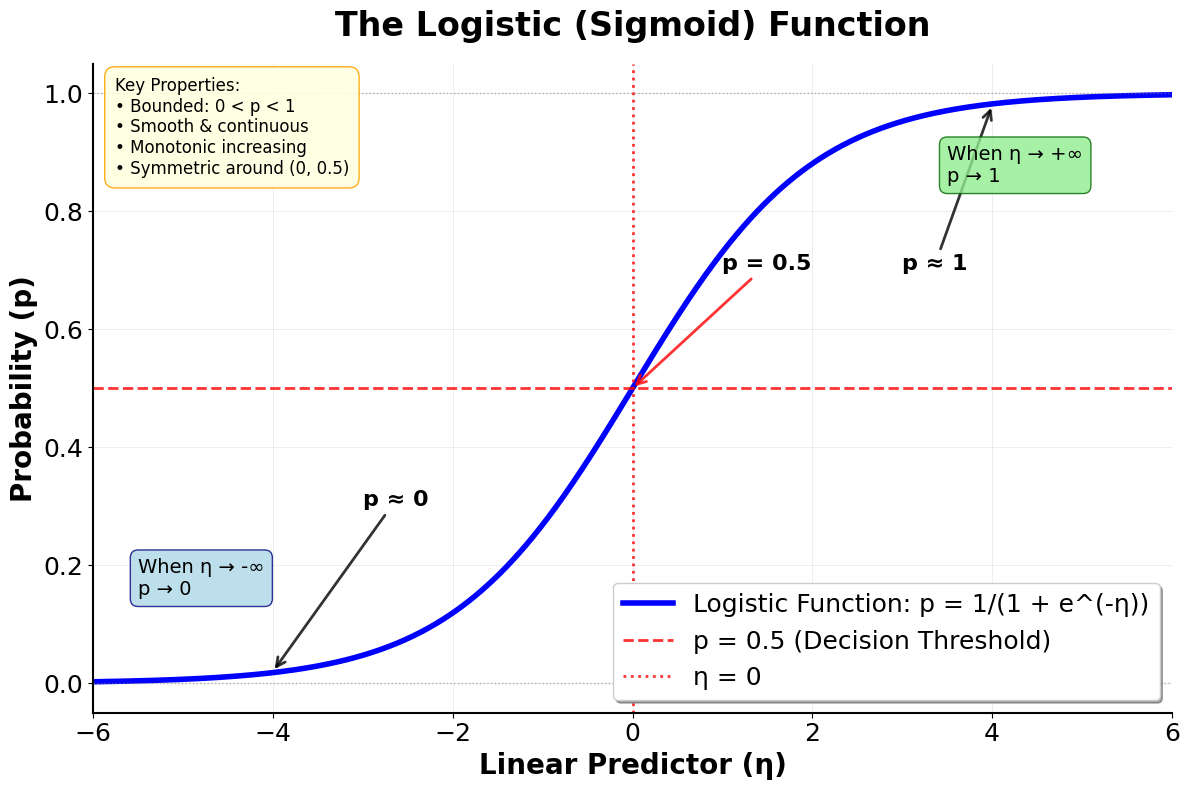
This visualization shows the characteristic S-shaped curve of the logistic function. Notice how:

At η = 0: The probability is exactly 0.5, and the curve is steepest here

As η becomes very negative: The probability approaches 0 asymptotically

As η becomes very positive: The probability approaches 1 asymptotically

The curve is smooth: No sharp corners or discontinuities, making optimization tractable

The curve is symmetric: Around the point (0, 0.5)

The Logit Function (Inverse of Logistic)

The logit function is the inverse of the logistic function and represents the log-odds:

$\text{logit}(p) = \log\left(\frac{p}{1-p}\right) = \eta$

where:

• $\text{logit}(p)$ is the logit function (transforms probabilities to log-odds)
• $p$ is the probability (bounded between 0 and 1)
• $\frac{p}{1-p}$ is the odds (the ratio of the probability of success to the probability of failure)
• $\log(\cdot)$ is the natural logarithm (base $e$)
• $\eta$ is the linear predictor (the right-hand side: $\beta_0 + \beta_1 x_1 + \cdots + \beta_p x_p$)

This equation reads as: "The log-odds of the probability equals the linear predictor."

Let's visualize this relationship to understand why logistic regression models the log-odds as a linear function:

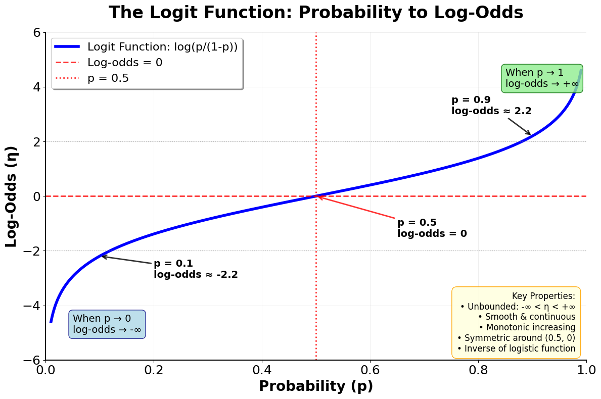
This visualization shows why logistic regression models the log-odds rather than the probability directly. The logit transformation converts probabilities (which are bounded between 0 and 1) into log-odds (which can be any real number from $-\infty$ to $+\infty$). This unbounded range makes it possible to use a linear model:

At p = 0.5: The log-odds are 0, representing equal odds for both outcomes

As p approaches 0: The log-odds approach $-\infty$, representing very low odds

As p approaches 1: The log-odds approach $+\infty$, representing very high odds

The relationship is smooth and monotonic: Higher probabilities correspond to higher log-odds

Complete Logistic Regression Model

Putting it all together, the complete logistic regression model is:

$\log\left(\frac{p}{1-p}\right) = \beta_0 + \beta_1 x_1 + \beta_2 x_2 + \cdots + \beta_p x_p$

where:

• $p = P(Y=1|X)$ is the probability that the response variable equals 1 given predictors $X$ (the parameter we're modeling)
• $\frac{p}{1-p}$ is the odds of success (the ratio of the probability of success to the probability of failure)
• $\log\left(\frac{p}{1-p}\right)$ is the log-odds or logit (the natural logarithm of the odds)
• $\beta_0$ is the intercept (the log-odds when all features equal zero)
• $\beta_1, \beta_2, \ldots, \beta_p$ are the regression coefficients (represent the change in log-odds for a one-unit increase in each feature)
• $x_1, x_2, \ldots, x_p$ are the feature values (predictor variables for a single observation)
• $p$ is the number of features (total count of predictor variables in the model)

This is read as: "The log-odds of the probability equals the linear combination of features."

Matrix Notation

In matrix form, logistic regression can be written as:

$\log\left(\frac{\mathbf{p}}{1-\mathbf{p}}\right) = \mathbf{X}\boldsymbol{\beta}$

where:

• $\mathbf{p}$ is the vector of predicted probabilities (an $n \times 1$ vector where each element is the predicted probability for one observation)
• $\mathbf{X}$ is the design matrix of features (an $n \times (p+1)$ matrix including a column of 1s for the intercept)
• $\boldsymbol{\beta}$ is the vector of coefficients (a $(p+1) \times 1$ vector containing the intercept and all feature coefficients)
• $n$ is the number of observations (rows in the dataset)
• $p$ is the number of features (excluding the intercept)
• The logit function $\log\left(\frac{\mathbf{p}}{1-\mathbf{p}}\right)$ is applied element-wise to $\mathbf{p}$

Mathematical Properties

Bounded Output: The logistic function ensures probabilities remain between 0 and 1

Smooth and Continuous: The function is differentiable everywhere, making optimization tractable

Symmetric: The function is symmetric around 0.5 when $\eta = 0$ (i.e., $p(0) = 0.5$)

Monotonic: As the linear predictor increases, the probability increases monotonically

Asymptotic: The function approaches 0 and 1 asymptotically without reaching them

Convex Log-likelihood: The negative log-likelihood is convex, ensuring a unique global maximum

Visualizing Logistic Regression

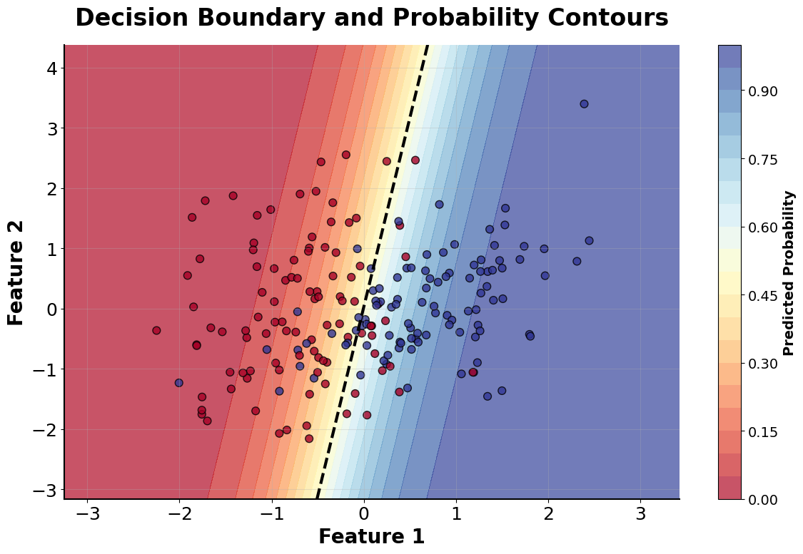
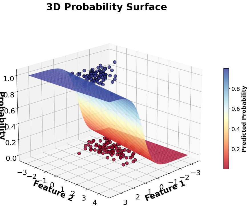
Let's create visualizations that show the key components of logistic regression. We'll start with the fundamental mathematical concepts and then explore the decision-making process.

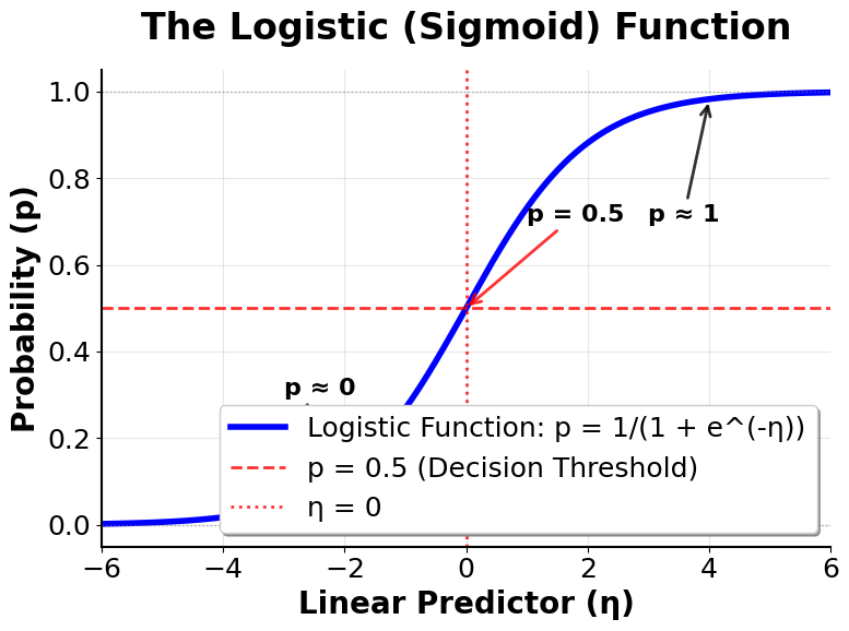
Now let's explore how logistic regression makes decisions in practice:

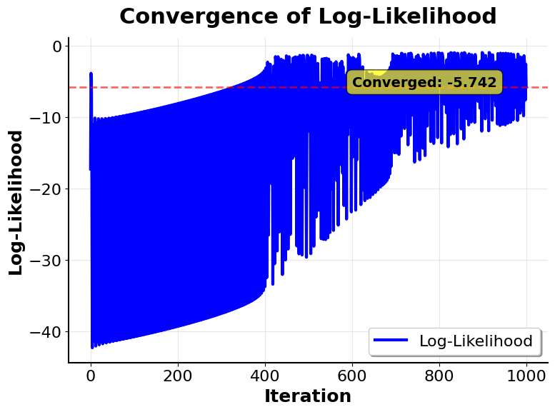
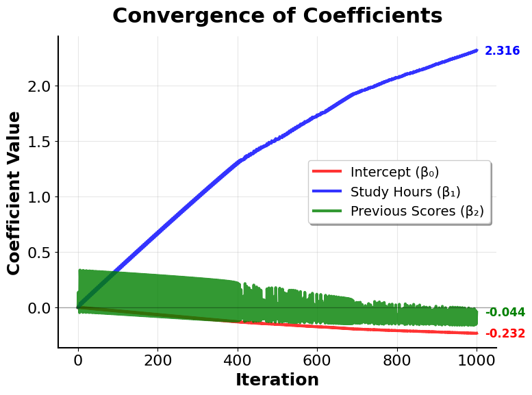
These visualizations demonstrate the iterative nature of logistic regression optimization:

Log-Likelihood Convergence: Shows how the model improves with each iteration, with rapid initial progress that gradually slows as it approaches the optimal solution. The log-likelihood is maximized (becomes less negative) as the model learns better parameters.

Coefficient Convergence: Illustrates how each coefficient evolves from its initial value to its final estimate. Different coefficients may converge at different rates depending on the data and feature scales. The convergence pattern shows that the optimization is working correctly: coefficients stabilize rather than oscillating or diverging.

Step 9: Final model interpretation

The fitted logistic regression model is:

$\log\left(\frac{p}{1-p}\right) = -15.2 + 0.8 \cdot \text{hours} + 0.1 \cdot \text{scores}$

where:

• $p$ is the probability of passing the exam (the outcome we're predicting)
• $\text{hours}$ is the number of study hours (feature $x_1$)
• $\text{scores}$ is the previous test score (feature $x_2$)

Interpretation:

Intercept ($\hat{\beta}_0 = -15.2$): When both study hours and previous scores are 0, the log-odds are -15.2, corresponding to a very low probability of passing

Study hours coefficient ($\hat{\beta}_1 = 0.8$): For each additional hour of study, the log-odds of passing increase by 0.8, holding previous scores constant

Previous scores coefficient ($\hat{\beta}_2 = 0.1$): For each additional point on previous scores, the log-odds of passing increase by 0.1, holding study hours constant

Step 10: Make predictions

For a student with 5 hours of study and a previous score of 75:

First, calculate the linear predictor:

$\eta = \hat{\beta}_0 + \hat{\beta}_1 \cdot \text{hours} + \hat{\beta}_2 \cdot \text{scores}$ $= -15.2 + 0.8 \cdot 5 + 0.1 \cdot 75$ $= -15.2 + 4.0 + 7.5$ $= -3.7$

Then, apply the logistic function to get the probability:

$p = \frac{1}{1 + e^{-\eta}} = \frac{1}{1 + e^{-(-3.7)}} = \frac{1}{1 + e^{3.7}}$

Since $e^{3.7} \approx 40.45$:

$p = \frac{1}{1 + 40.45} = \frac{1}{41.45} \approx 0.024$

This student has approximately a 2.4% chance of passing.

For a student with 7 hours of study and a previous score of 85:

First, calculate the linear predictor:

$\eta = -15.2 + 0.8 \cdot 7 + 0.1 \cdot 85$ $= -15.2 + 5.6 + 8.5$ $= -1.1$

Then, apply the logistic function:

$p = \frac{1}{1 + e^{-(-1.1)}} = \frac{1}{1 + e^{1.1}}$

Since $e^{1.1} \approx 3.00$:

$p = \frac{1}{1 + 3.00} = \frac{1}{4.00} = 0.25$

This student has a 25% chance of passing.

Implementation

This section demonstrates how to implement logistic regression using scikit-learn with proper preprocessing, evaluation, and interpretation of results.

Basic Implementation

We'll start by creating a synthetic dataset that simulates student exam outcomes based on study hours and previous test scores. This example demonstrates the complete workflow from data preparation through model evaluation.

Now we'll create a pipeline that combines feature scaling with logistic regression. Using a pipeline ensures that preprocessing steps are applied consistently during both training and prediction.

Model Performance

Let's evaluate the model's performance using multiple metrics to get a comprehensive understanding of how well it performs.

The accuracy of approximately 0.81 indicates that the model correctly classifies about 81% of test cases. The ROC AUC score of around 0.88 demonstrates strong discriminative ability—the model effectively separates the two classes across different probability thresholds. An AUC above 0.85 is generally considered good performance, suggesting the model has learned meaningful patterns from the training data.

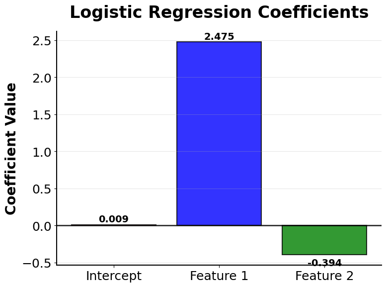
Model Coefficients

The learned coefficients reveal how each feature influences the probability of passing.

The positive coefficients for both study hours and previous scores confirm our intuition—more study time and higher previous scores both increase the probability of passing. Since we standardized the features, these coefficients are directly comparable. The study hours coefficient is larger in magnitude, suggesting it has a stronger influence on the outcome than previous scores in this dataset.

Sample Predictions

Let's examine predictions for a few individual students to see how the model assigns probabilities.

These individual predictions show how the model translates feature values into probabilities. Notice that students with higher study hours and scores receive higher probabilities of passing. The model provides nuanced probability estimates rather than just binary predictions, which is valuable for understanding confidence in each prediction.

Detailed Evaluation Metrics

The classification report provides precision, recall, and F1-scores for each class, giving us deeper insight into model performance.

The classification report shows balanced performance across both classes. Precision indicates how many predicted passes were actually passes, while recall shows how many actual passes were correctly identified. The F1-score balances both metrics. The macro and weighted averages around 0.81 indicate consistent performance across both classes without significant bias toward either.

The confusion matrix shows the breakdown of correct and incorrect predictions. The diagonal elements represent correct predictions (true negatives and true positives), while off-diagonal elements show misclassifications. A well-performing model has most predictions concentrated on the diagonal.

Cross-Validation

Cross-validation provides a more robust estimate of model performance by evaluating on multiple train-test splits.

The cross-validation scores show consistent performance across all five folds, with a mean AUC around 0.88. The small standard deviation indicates that the model's performance is stable and not dependent on a particular train-test split. This consistency suggests the model will generalize well to new data.

Polynomial Features Extension

For datasets with non-linear relationships, we can extend logistic regression by adding polynomial features to capture interactions and curved patterns.

In this example, adding polynomial features does not substantially improve performance because the underlying relationship is already approximately linear. The minimal improvement (less than 1%) likely reflects random variation rather than genuine model enhancement. However, for datasets with true non-linear patterns or important feature interactions, polynomial features can provide significant performance gains. Use cross-validation to determine whether the added complexity is justified by improved generalization.

Key Parameters

Below are the main parameters that control how logistic regression works and performs.

• penalty: Type of regularization to apply (default: 'l2'). Options include 'l1' (Lasso), 'l2' (Ridge), 'elasticnet', or 'none'. L1 performs feature selection, L2 handles multicollinearity, and elasticnet combines both.
• C: Inverse of regularization strength (default: 1.0). Smaller values specify stronger regularization. Values like 0.01 prevent overfitting with many features, while values like 10 or 100 allow closer fitting to training data. Typical range: [0.001, 0.01, 0.1, 1, 10, 100].
• solver: Algorithm for optimization (default: 'lbfgs'). Options include 'lbfgs' (good default), 'liblinear' (for small datasets), 'sag' and 'saga' (for large datasets), and 'newton-cg'. The 'saga' solver supports all penalty types.
• max_iter: Maximum number of iterations for convergence (default: 100). Increase to 1000 or more if you encounter convergence warnings. More iterations allow the optimizer more time to find the optimal solution.
• class_weight: Weights for classes (default: None). Set to 'balanced' to automatically adjust weights inversely proportional to class frequencies, which helps with imbalanced datasets.
• random_state: Seed for reproducibility (default: None). Set to an integer to ensure consistent results across runs, which is important for debugging and comparison.
• n_jobs: Number of CPU cores to use for parallel computation (default: None). Set to -1 to use all available cores, which speeds up cross-validation.

Key Methods

The following are the most commonly used methods for working with logistic regression models.

• fit(X, y): Trains the logistic regression model on training data X and target labels y. This method learns the optimal coefficients through maximum likelihood estimation.
• predict(X): Returns predicted class labels (0 or 1) for input data X using the default 0.5 probability threshold. Use this when you need binary classifications.
• predict_proba(X): Returns probability estimates for each class. The output is an array where each row contains [probability of class 0, probability of class 1]. Use this when you need probability scores or want to apply custom thresholds.
• predict_log_proba(X): Returns log-probabilities for each class, which can be useful for numerical stability in certain applications or when working with log-likelihood calculations.
• score(X, y): Returns the mean accuracy on the given test data and labels. This is a convenience method that combines prediction and accuracy calculation.
• decision_function(X): Returns the signed distance of samples to the decision boundary (the linear predictor η before applying the logistic function). Useful for understanding how confident predictions are.

Practical Applications

Practical Implications

Logistic regression is particularly valuable for binary classification problems where interpretability and computational efficiency are important. In medical diagnosis, logistic regression excels at predicting disease presence based on symptoms and test results because healthcare professionals need to understand which factors contribute most to the diagnosis. The model's coefficients provide clear insights into how each biomarker or symptom influences the probability of disease, making it suitable for clinical decision support systems where transparency is required.

In finance and credit risk assessment, logistic regression is widely used for loan default prediction and credit approval decisions. Financial institutions value the model's interpretability because they need to explain their decisions to regulators and customers. The algorithm's ability to provide probability estimates rather than binary predictions allows for risk-based pricing and decision-making, where different thresholds can be applied based on risk tolerance. Similarly, in fraud detection, logistic regression serves as an effective baseline model that can process transactions in real-time while providing interpretable risk scores.

Marketing applications benefit from logistic regression's probability outputs for customer behavior prediction, such as purchase likelihood, campaign response, or churn prediction. The model's efficiency makes it suitable for scoring large customer databases, while the interpretable coefficients help marketing teams understand which customer attributes drive conversion. In quality control and manufacturing, logistic regression can predict product defects based on manufacturing parameters, helping identify which process variables most strongly influence quality outcomes.

Best Practices

For hyperparameter tuning, focus on the regularization parameter C, which controls the trade-off between model complexity and generalization. Start with the default value of C=1.0 and use cross-validation to explore values in the range [0.001, 0.01, 0.1, 1, 10, 100]. Lower C values (e.g., 0.01) apply stronger regularization and work well when you have many features or suspect overfitting, while higher values (e.g., 10 or 100) allow the model to fit the training data more closely. Choose between L1 regularization (penalty='l1') for automatic feature selection when you have many potentially irrelevant features, or L2 regularization (penalty='l2') for better numerical stability when features are correlated.

Use cross-validation to evaluate model performance rather than relying on a single train-test split, as this provides more robust estimates of generalization performance. Set random_state for reproducibility in both data splitting and model initialization. When evaluating your model, use multiple metrics appropriate to your problem: ROC AUC for overall discriminative ability, precision and recall when false positives and false negatives have different costs, and log-loss when probability calibration is important. For imbalanced datasets, use stratify=y in train_test_split to maintain class proportions, and consider using class_weight='balanced' to automatically adjust for class imbalance during training.

Use pipelines from scikit-learn to combine preprocessing and modeling steps, which prevents data leakage and ensures consistent transformations between training and deployment. This approach also simplifies model deployment by packaging all necessary transformations with the model itself. When working with new data, always apply the same preprocessing steps in the same order to maintain consistency with the training process.

Data Requirements and Preprocessing

Logistic regression requires complete data without missing values, as the algorithm cannot process observations with undefined features. Handle missing data through imputation (mean, median, or mode for numerical features; most frequent category for categorical features), or remove observations with missing values if the missingness is random and you have sufficient data. For systematic missingness patterns, consider creating indicator variables to flag missing values, as the missingness itself may be informative.

Categorical variables need to be converted to numerical format before training. Use one-hot encoding for nominal variables without inherent order (such as product categories or geographic regions), which creates binary indicator variables for each category. For ordinal variables with meaningful order (such as education level or satisfaction ratings), label encoding preserves the ordinal relationship. When dealing with high-cardinality categorical variables (many unique categories), consider target encoding or grouping rare categories to prevent creating too many features. Be cautious with one-hot encoding when categories have very few observations, as this can lead to unstable coefficient estimates.

Feature scaling using StandardScaler improves numerical stability during optimization and makes coefficients directly comparable across features. While logistic regression does not strictly require scaling like distance-based algorithms, standardization is particularly beneficial when features have different units or magnitudes. The algorithm assumes linear relationships between features and log-odds of the outcome, which may not hold for all variables. Examine your features for non-linear patterns using exploratory data analysis and consider applying transformations such as logarithms for right-skewed distributions, square roots for count data, or polynomial features for variables with curved relationships. Create interaction terms when you suspect that the effect of one feature depends on the value of another.

Common Pitfalls

One frequent mistake is neglecting class imbalance in the training data. When one class is much more common than the other (for example, fraud cases representing less than 1% of transactions), the model may achieve high accuracy by simply predicting the majority class for all observations, resulting in poor recall for the minority class. Address this by using class_weight='balanced' to automatically adjust the loss function, or by resampling techniques such as SMOTE for oversampling the minority class or random undersampling of the majority class. Note that stratify=y in train_test_split only maintains class proportions in splits and does not address the underlying imbalance.

Another common issue is using the default 0.5 probability threshold without considering the specific costs of false positives versus false negatives. In many applications, these errors have different consequences. For example, in medical screening, false negatives (missing a disease) may be more costly than false positives (unnecessary follow-up tests). Adjust the decision threshold based on your evaluation metric and business requirements. Use precision-recall curves or ROC curves to identify optimal thresholds, recognizing that the threshold maximizing F1-score often differs from 0.5, especially with imbalanced data.

Failing to regularize the model when you have many features relative to the number of observations can lead to overfitting, where the model memorizes training data patterns that fail to generalize. This is particularly problematic when features are correlated or when using polynomial or interaction features. Apply L1 or L2 regularization and tune the C parameter using cross-validation. Including highly correlated features without regularization can lead to unstable coefficient estimates where small changes in the data produce large changes in coefficients. Use correlation analysis or variance inflation factors (VIF) to identify and remove redundant features, or rely on L2 regularization to handle multicollinearity.

Computational Considerations

Logistic regression has computational complexity of O(n × p) per iteration for n observations and p features, with the number of iterations depending on convergence criteria and optimization algorithm. For typical datasets (up to 100,000 observations and 1,000 features), training completes in seconds on modern hardware. The algorithm scales well to larger datasets because the optimization problem is convex with a unique global optimum, and efficient solvers like L-BFGS or SAG (Stochastic Average Gradient) converge quickly.

For very large datasets (millions of observations), consider using the solver='sag' or solver='saga' options in scikit-learn, which are optimized for large-scale problems and converge faster than the default L-BFGS solver. These solvers use stochastic gradient descent variants that process data in mini-batches, reducing memory requirements. If your dataset doesn't fit in memory, consider using online learning approaches with partial_fit() or sampling strategies to train on representative subsets. When you have many features (tens of thousands), L1 regularization with penalty='l1' and solver='saga' can perform automatic feature selection, reducing both model complexity and prediction time.

Memory requirements are generally modest, as the model only needs to store p coefficients plus the optimization state. Prediction is extremely fast with O(p) complexity per observation, making logistic regression suitable for real-time applications requiring low-latency predictions. For deployment in production systems with high throughput requirements, the model can easily handle thousands of predictions per second on standard hardware. When computational resources are constrained, logistic regression's efficiency makes it preferable to more complex models like gradient boosting or neural networks that require significantly more computation for both training and inference.

Performance and Deployment Considerations

Evaluate logistic regression performance using metrics appropriate to your problem and business objectives. For balanced datasets, accuracy provides a reasonable overall measure, but for imbalanced data, focus on precision, recall, F1-score, and ROC AUC. Precision measures the proportion of positive predictions that are correct, which is important when false positives are costly. Recall measures the proportion of actual positives that are correctly identified, which is important when false negatives are costly. ROC AUC evaluates discriminative ability across all possible thresholds, providing a threshold-independent performance measure. Use log-loss (cross-entropy) when probability calibration is important, as it penalizes confident incorrect predictions more heavily than accuracy.

Calibration of predicted probabilities is important for applications where the probability values themselves are used for decision-making rather than the binary predictions. Check calibration using reliability diagrams (calibration plots) that compare predicted probabilities to observed frequencies. Well-calibrated models have predicted probabilities that match true probabilities—for example, among observations predicted with 70% probability, approximately 70% should belong to the positive class. If calibration is poor, apply calibration techniques such as Platt scaling or isotonic regression using scikit-learn's CalibratedClassifierCV.

For deployment, logistic regression offers advantages due to its simplicity and efficiency. The model serializes easily using pickle or joblib, and the small model size (the coefficient vector) makes it suitable for edge deployment or embedding in applications. Ensure you save the entire pipeline including preprocessing steps, rather than the model alone, to maintain consistency between training and prediction. Monitor model performance in production by tracking prediction distributions, feature distributions, and evaluation metrics over time. Concept drift (where the relationship between features and target changes) can degrade performance, so implement monitoring to detect when retraining is needed. Set up alerts for changes in prediction distribution or feature statistics, and establish a retraining schedule based on how quickly your data patterns evolve.

Summary

Logistic regression is a fundamental and powerful classification algorithm that models the probability of binary outcomes using the logistic function. By transforming a linear combination of features into probabilities bounded between 0 and 1, logistic regression provides both interpretable results and reliable predictions for a wide range of binary classification problems.

The key strength of logistic regression lies in its simplicity and interpretability. The coefficients have clear meanings—they represent the change in log-odds for a one-unit increase in the corresponding feature—making it easy to understand which features are most important and how they influence the outcome. This interpretability, combined with computational efficiency and good performance on many real-world problems, makes logistic regression an important tool in the data scientist's toolkit.

However, logistic regression's linearity assumption can be a limitation when dealing with complex, non-linear relationships in the data. While feature engineering techniques like polynomial features can help address this limitation, there are cases where more complex algorithms might be more appropriate. Additionally, the method's sensitivity to outliers and potential struggles with imbalanced datasets require careful preprocessing and evaluation.

Despite these limitations, logistic regression remains one of the most widely used algorithms in machine learning, serving as an excellent baseline model and often providing surprisingly good results. Its combination of interpretability, efficiency, and effectiveness makes it particularly valuable in applications where understanding the model's decisions is as important as the predictions themselves, such as in healthcare, finance, and other regulated industries.