

Master DBSCAN (Density-Based Spatial Clustering of Applications with Noise), the algorithm that discovers clusters of any shape without requiring predefined cluster counts. Learn core concepts, parameter tuning, and practical implementation.

This article is part of the free-to-read Machine Learning from Scratch
Choose your expertise level to adjust how many terms are explained. Beginners see more tooltips, experts see fewer to maintain reading flow. Hover over underlined terms for instant definitions.
DBSCAN (Density-Based Spatial Clustering of Applications with Noise)
DBSCAN is a density-based clustering algorithm that groups together points that are closely packed together, marking as outliers points that lie alone in low-density regions. Unlike k-means clustering, which assumes spherical clusters and requires us to specify the number of clusters beforehand, DBSCAN automatically determines the number of clusters based on the density of data points and can identify clusters of arbitrary shapes.
The algorithm works by defining a neighborhood around each point and then connecting points that are sufficiently close to each other. If a point has enough neighbors within its neighborhood, it becomes a "core point" and can form a cluster. Points that are reachable from core points but don't have enough neighbors themselves become "border points" of the cluster. Points that are neither core nor border points are classified as "noise" or outliers.
This density-based approach makes DBSCAN particularly effective for datasets with clusters of varying densities and shapes, and it naturally handles noise and outliers without requiring them to be assigned to any cluster. The algorithm is especially valuable in applications where we don't know the number of clusters in advance and where clusters may have irregular, non-spherical shapes.
Advantages
DBSCAN excels at finding clusters of arbitrary shapes, making it much more flexible than centroid-based methods like k-means. While k-means assumes clusters are roughly spherical and similar in size, DBSCAN can discover clusters that are elongated, curved, or have complex geometries. This makes it particularly useful for spatial data analysis, image segmentation, and any domain where clusters don't conform to simple geometric shapes.
The algorithm automatically determines the number of clusters without requiring us to specify this parameter beforehand. This is a significant advantage over methods like k-means, where choosing the wrong number of clusters can lead to poor results. DBSCAN discovers the natural number of clusters based on the density structure of the data, making it more robust for exploratory data analysis.
DBSCAN has built-in noise detection capabilities, automatically identifying and separating outliers from the main clusters. This is particularly valuable in real-world datasets where noise and outliers are common. Unlike other clustering methods that force every point into a cluster, DBSCAN can leave some points unassigned, which often reflects the true structure of the data more accurately.
Disadvantages
DBSCAN struggles with clusters of varying densities within the same dataset. The algorithm uses global parameters (eps and min_samples) that apply uniformly across the entire dataset. If one region of the data has much higher density than another, DBSCAN may either miss the sparse clusters (if eps is too small) or merge distinct dense clusters (if eps is too large). This limitation can be problematic in datasets where clusters naturally have different density characteristics.
The algorithm is sensitive to the choice of its two main parameters: eps (the maximum distance between two samples for one to be considered in the neighborhood of the other) and min_samples (the minimum number of samples in a neighborhood for a point to be considered a core point). Choosing appropriate values for these parameters often requires domain knowledge and experimentation, and poor parameter choices can lead to either too many small clusters or too few large clusters.
DBSCAN can be computationally expensive for large datasets, especially when using the brute-force approach for nearest neighbor searches. While optimized implementations exist, the algorithm's time complexity can still be problematic for very large datasets. Additionally, the algorithm doesn't scale well to high-dimensional data due to the curse of dimensionality, where distance metrics become less meaningful as the number of dimensions increases.
Formula
Traditional clustering algorithms like k-means operate under a comforting but often false assumption: that clusters are roughly spherical and similar in size. These methods place cluster centers and assign each point to the nearest center, drawing clean circular boundaries around groups of data. But real-world data rarely cooperates with such geometric idealism.
Consider the challenge of identifying neighborhoods in a city. Some neighborhoods wind along riverbanks. Others sprawl across irregular terrain. A few cluster tightly around transit hubs while others stretch along major roads. No amount of circular boundaries will capture these organic shapes. We need a fundamentally different approach, one that asks not "where are the centers?" but rather "where are the crowds?"
This shift in perspective, from centers to density, is the foundational insight behind DBSCAN. Instead of imposing geometric constraints, we let the data reveal its own structure by following the natural concentrations of points.
From City Streets to Mathematical Rigor
Imagine wandering through a sprawling city at night, trying to identify distinct neighborhoods based on where people naturally congregate. You notice some areas buzzing with activity: crowded bars, street performers, food trucks. Others remain quiet and sparsely populated. Traditional approaches might simply draw circles around the busiest intersections and call those "neighborhoods," but this misses something fundamental about how real communities form.
What if, instead of assuming neighborhoods are perfectly circular regions around central points, we asked: "Where do people actually gather, and how can we follow the natural paths of activity from one lively spot to another?" This density-based perspective allows us to discover neighborhoods of any conceivable shape, whether winding streets, irregular blocks, or sprawling districts, by tracing the organic flow of human activity.
DBSCAN embodies this intuition mathematically. It doesn't impose artificial geometric constraints on clusters. Instead, it asks the data: "Where are the natural gathering places, and how do they connect?" This approach reveals clusters that match reality rather than forcing reality to fit our preconceptions.
The mathematical framework we're about to construct transforms this intuitive city-walking metaphor into rigorous, executable definitions. We'll build it systematically through four progressive layers:
| Layer | Question Answered | Mathematical Tool |
|---|---|---|
| Proximity | Which points are close to each other? | The ε-neighborhood |
| Density | Which regions are crowded enough to matter? | Core point criterion |
| Reachability | How do dense regions connect? | Density-reachability chains |
| Connectivity | Which points belong to the same cluster? | Density-connectivity |
This progression mirrors how we naturally understand neighborhoods: first we notice proximity, then density, then connection, and finally belonging. Let's embark on this journey together.
The Epsilon-Neighborhood: Defining "Nearby"
Every clustering algorithm must answer a fundamental question: how do we determine which points are "close enough" to potentially belong together? In our city exploration metaphor, this is equivalent to deciding how far you need to walk to consider two locations part of the same neighborhood. The challenge is that "close" means different things in different contexts: a block in Manhattan feels very different from a block in rural Kansas.
DBSCAN's solution is elegantly simple: draw a circle around each point with a fixed radius called eps (epsilon), and consider all points within that circle as "neighbors." This creates a consistent, scale-invariant definition of proximity that works across different datasets and dimensions.
The circular neighborhood captures our intuitive understanding that proximity should be symmetric: if point A is close to point B, then point B should automatically be close to point A. The circle also creates a smooth, continuous definition of closeness that doesn't introduce artificial boundaries or corners. In our city metaphor, it's like asking "who lives within walking distance?" rather than "who lives within these rigid geometric boundaries?"
For any point in our dataset , we define its epsilon-neighborhood as the set of all points within distance eps:
Let's unpack each component of this definition:
- is the neighborhood of point with radius eps, essentially 's "personal space" in the data. The subscript reminds us that this neighborhood depends on our choice of eps.
- is our complete dataset of points, the universe from which we're selecting neighbors.
- represents any candidate point we're testing for membership. The notation means "for each point in the dataset ."
- is our proximity test: the distance between and must not exceed eps.
- denotes set notation. We're collecting all points that pass the proximity test into a single set.
The distance function measures how far apart two points are. While DBSCAN works with any valid distance metric, the most common choice is Euclidean distance:
This is simply the Pythagorean theorem applied to two-dimensional coordinates: the straight-line distance between points and . In higher dimensions, we sum the squared differences across all coordinates before taking the square root.
The eps parameter becomes our first design choice. A larger eps creates bigger neighborhoods, making it easier for points to connect and form larger clusters. A smaller eps creates more selective neighborhoods, leading to tighter, more distinct clusters. This parameter fundamentally controls how "generous" our definition of "nearby" will be in the clustering process.
But here's a crucial insight that separates mere proximity from genuine clustering: just because two points are neighbors doesn't mean they belong to the same cluster. You could stand next to someone on a crowded subway platform during rush hour, but you're not part of the same social group or community. We need a mechanism to distinguish between coincidental proximity and genuine community membership.
This distinction leads us to the core innovation of DBSCAN: density.
Core Points: Identifying Dense Regions
Proximity alone isn't enough. Now we face a second fundamental question: what distinguishes a "genuinely crowded area" from "just a few random points that happen to be nearby"? This distinction is crucial because not every group of nearby points deserves to be called a cluster.
Let's return to our city metaphor. Imagine walking through the city at night and passing through different areas:
- A quiet street corner: Just you and one other person waiting for a bus. This isn't a neighborhood gathering; it's just coincidental proximity.
- A busy restaurant district: Dozens of people at outdoor tables, street performers, pedestrians moving between venues. This feels like a vibrant community hub where activity naturally concentrates.
The difference isn't merely about counting people. It's about density, the concentration of activity in a specific area that creates a genuine social space. The restaurant district has enough people packed together that it becomes a destination in itself. The bus stop? That's just two people who happen to be waiting at the same time.
DBSCAN formalizes this intuition through the concept of a core point: a point that sits at the heart of a sufficiently dense region. Core points become the anchor points around which clusters form, much like popular restaurants or bars that draw crowds and ultimately define neighborhood boundaries.
A core point is a data point that has at least min_samples neighbors (including itself) within its eps-neighborhood. Core points form the "backbone" of clusters, the dense regions from which cluster membership propagates outward.
The "sufficiently dense" criterion is controlled by our second parameter, min_samples. A point becomes a core point if it has at least min_samples neighbors (including itself) within its eps-neighborhood. Think of min_samples as our "crowded enough" threshold, the minimum population needed before we consider an area a genuine social hub rather than random coincidence.
The mathematical definition captures this with elegant simplicity:
This inequality asks a single, decisive question: "Does point have enough neighbors to be considered part of a dense region?" Let's break down each term:
- is the cardinality (count) of the neighborhood. The vertical bars denote "size of," so this gives us the total number of points within eps distance of , including itself. If has three neighbors plus itself, this equals 4.
- is our density threshold parameter, the minimum population required.
- is the inequality test. If the neighborhood size meets or exceeds our threshold, qualifies as a core point.
Why this threshold matters. Without min_samples, any two nearby points would form a cluster, creating meaningless micro-communities everywhere. With min_samples, we ensure that only genuinely dense regions have the power to spawn clusters. This leads to a natural three-way classification:
| Point Type | Criterion | Role in Clustering |
|---|---|---|
| Core point | Forms the dense backbone of clusters | |
| Border point | Has fewer than min_samples neighbors but lies within a core point's neighborhood | Belongs to a cluster but can't expand it |
| Noise point | Too few neighbors AND not reachable from any core point | Doesn't belong to any cluster |
The interplay of parameters. The eps and min_samples parameters work together like dance partners. Changing one affects what the other can accomplish:
| Scenario | Effect on Clustering |
|---|---|
| Large eps, low min_samples | Larger, more inclusive clusters; may merge distinct groups |
| Large eps, high min_samples | Moderate clusters; requires genuinely dense regions |
| Small eps, low min_samples | Many small, tight clusters; sensitive to local structure |
| Small eps, high min_samples | Very restrictive; most points become noise |
Together, these parameters define what we mean by local density: "A region is dense if it contains at least min_samples points within eps distance." This local approach, rather than relying on global statistics, allows DBSCAN to discover clusters even when different regions of the data have different natural densities.
Visualizing Neighborhoods and Core Points
The mathematical definitions become clearer when we see them geometrically. Let's visualize how DBSCAN classifies points based on their neighborhoods:
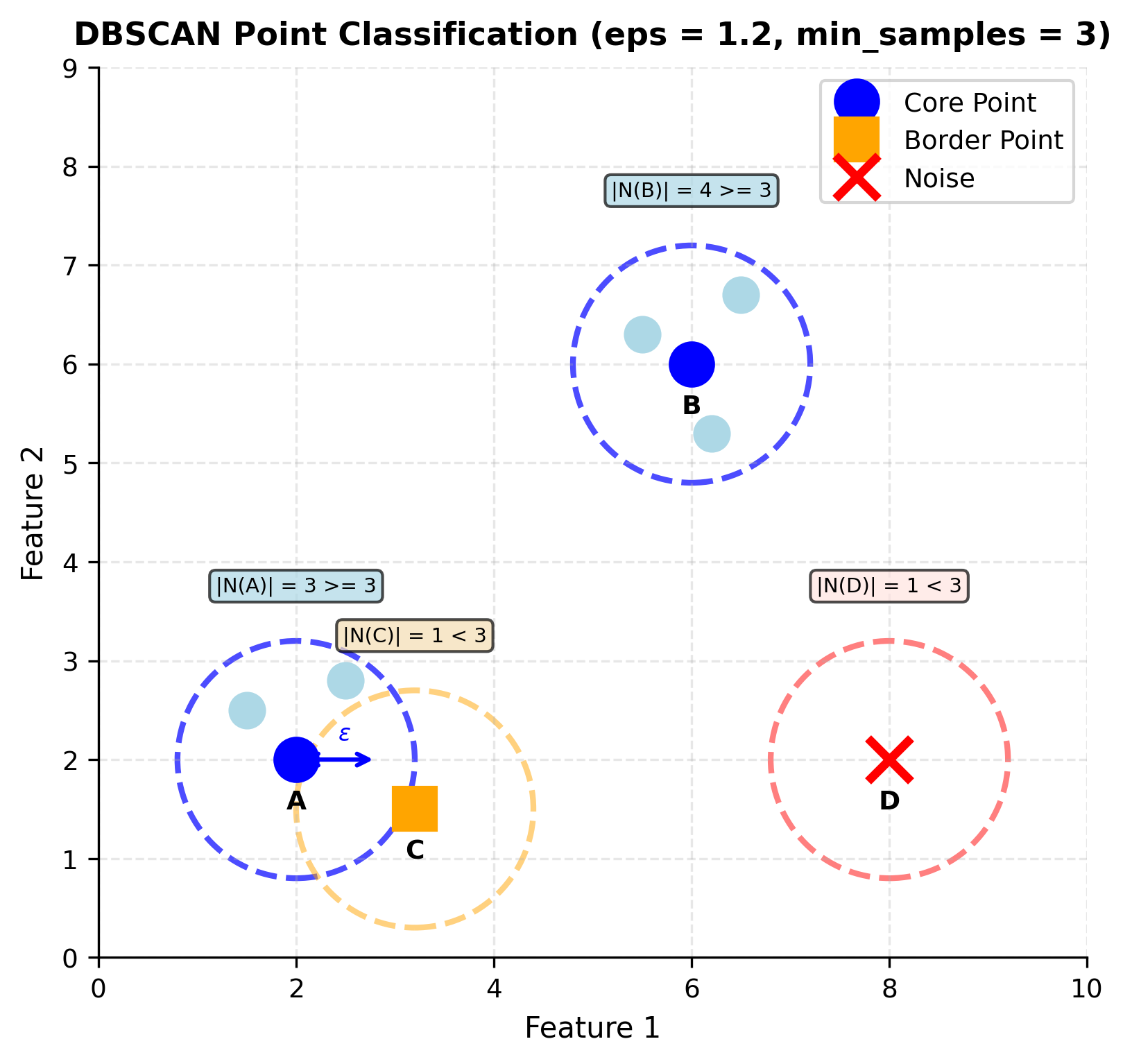
The dashed circles represent the ε-neighborhood for each point. Core points (blue circles) have neighborhoods containing at least min_samples points, satisfying . Border points (orange square) don't meet this threshold themselves but fall within a core point's neighborhood. Noise points (red X) satisfy neither condition; they're isolated in sparse regions of the data space.
Density-Reachability: Connecting Dense Regions
We now have core points that mark dense regions, but we face the algorithm's most elegant challenge: how do we connect these dense regions into cohesive clusters? Real communities don't exist in isolation. They link together through chains of activity and movement that create larger social networks.
Imagine our city has several vibrant districts, each with its own core of activity. But these districts aren't separate islands; people naturally flow between them, creating pathways that connect different neighborhoods. A coffee shop in one district might draw people from a nearby restaurant in another district. These connections create larger community networks that transcend individual gathering spots.
If we only connected points that are directly within each other's neighborhoods, we'd create isolated pockets, separate islands of density with no way to merge them. But real communities flow and merge. Two distant points might legitimately belong to the same larger neighborhood if they're connected through a chain of busy areas, even if they're not directly adjacent.
Think of navigating a crowded city by following the natural flow of people. You can reach any destination by stepping from one busy area to the next, as long as each step takes you to a sufficiently crowded spot. The path doesn't need to be straight; it can curve around parks, follow winding streets, or zigzag through alleyways. This organic movement, not rigid geometric rules, defines the true boundaries of neighborhoods.
DBSCAN formalizes this intuition through density-reachability: the principle that you can reach one point from another by following a chain of core points, where each step stays within someone's eps-neighborhood.
A point is directly density-reachable from point if two conditions hold: (1) is within 's eps-neighborhood, and (2) is a core point. This asymmetric relationship forms the building blocks of cluster connectivity.
The mathematical formulation captures both requirements in a single statement:
Let's unpack this formula:
- is the proximity requirement: point must lie within eps distance of point . This is the "within walking distance" part.
- is the density anchor requirement: must be a core point. You can only "step from" a busy area.
- is the logical AND operator, requiring both conditions to be true simultaneously.
- means "if and only if". The relationship holds exactly when both conditions are met.
Why require a core point anchor? Without this restriction, you could "jump" across sparse areas using border points as stepping stones. This would artificially connect separate communities through their outskirts, like claiming two distant suburbs are the same neighborhood just because their borders happen to touch. By requiring steps to originate from dense core regions, we ensure that cluster connections follow genuine pathways of activity.
From single steps to full paths. Direct density-reachability gives us single steps; we extend this to full paths through density-reachability. A point is density-reachable from if there exists a chain of points where each is directly density-reachable from :
This transitivity is what allows clusters to curve and bend naturally, following the organic contours of the data. A crescent moon-shaped cluster becomes possible because you can walk along its curved edge, stepping from one core point to the next. Traditional clustering would try to fit a circle or sphere around such data; DBSCAN traces the winding path that defines the true boundary.
Density-Connectivity: When Points Belong Together
Density-reachability gives us a powerful way to trace paths through dense regions, but it creates an awkward asymmetry. Point A might be reachable from point B, but B might not be reachable from A (if B isn't a core point). For deciding who belongs to which neighborhood, we need a relationship that works both ways, a symmetric definition of belonging.
Consider the problem: if we're building a neighborhood directory, the relationship "lives in the same neighborhood as" should be symmetric by nature. If I live in your neighborhood, then you must live in mine. One-directional relationships create confusion and arbitrary distinctions.
The solution is elegant: two points belong to the same cluster if they share a common anchor point, a "neighborhood center" from which both can be reached through density paths. This creates a symmetric relationship based on shared membership in the same community network, regardless of which point you start from.
Two points and are density-connected if there exists some core point from which both and are density-reachable. This symmetric relationship defines cluster membership: all points that are density-connected belong to the same cluster.
The mathematical formulation is:
Here's what each component means:
- means "there exists some point " that serves as their common anchor. This is the existential quantifier: we only need to find one such anchor point for the relationship to hold.
- and are density-reachable from means both points can be reached from through chains of directly density-reachable steps.
- indicates equivalence: the points are density-connected if and only if such an anchor exists.
Why this works beautifully. Cluster membership is based on genuine connectivity through dense regions. Points don't need to be directly connected to each other; they just need to be part of the same network of activity flowing from a common core. The symmetry emerges naturally: if both points trace back to the same origin, neither is "more connected" than the other.
Think of each cluster as a tree growing from an anchor point (the trunk). All leaves and branches belong to the same tree because they all connect back to the same trunk, regardless of which leaf you start from. Two leaves on different trees aren't connected, even if those trees grow close together.
The following table summarizes the mathematical relationships we've constructed:
| Relationship | Definition | Symmetric? | Purpose |
|---|---|---|---|
| Neighborhood | Points within eps distance | Yes | Define "nearby" |
| Core point | Has ≥ min_samples neighbors | N/A | Identify dense regions |
| Direct density-reachable | In neighborhood of core point | No | Single-step connections |
| Density-reachable | Chain of direct connections | No | Multi-step paths |
| Density-connected | Share common anchor | Yes | Cluster membership |
Visualizing Density-Reachability and Connectivity
To understand how DBSCAN forms clusters through density-reachability chains, let's visualize the process:
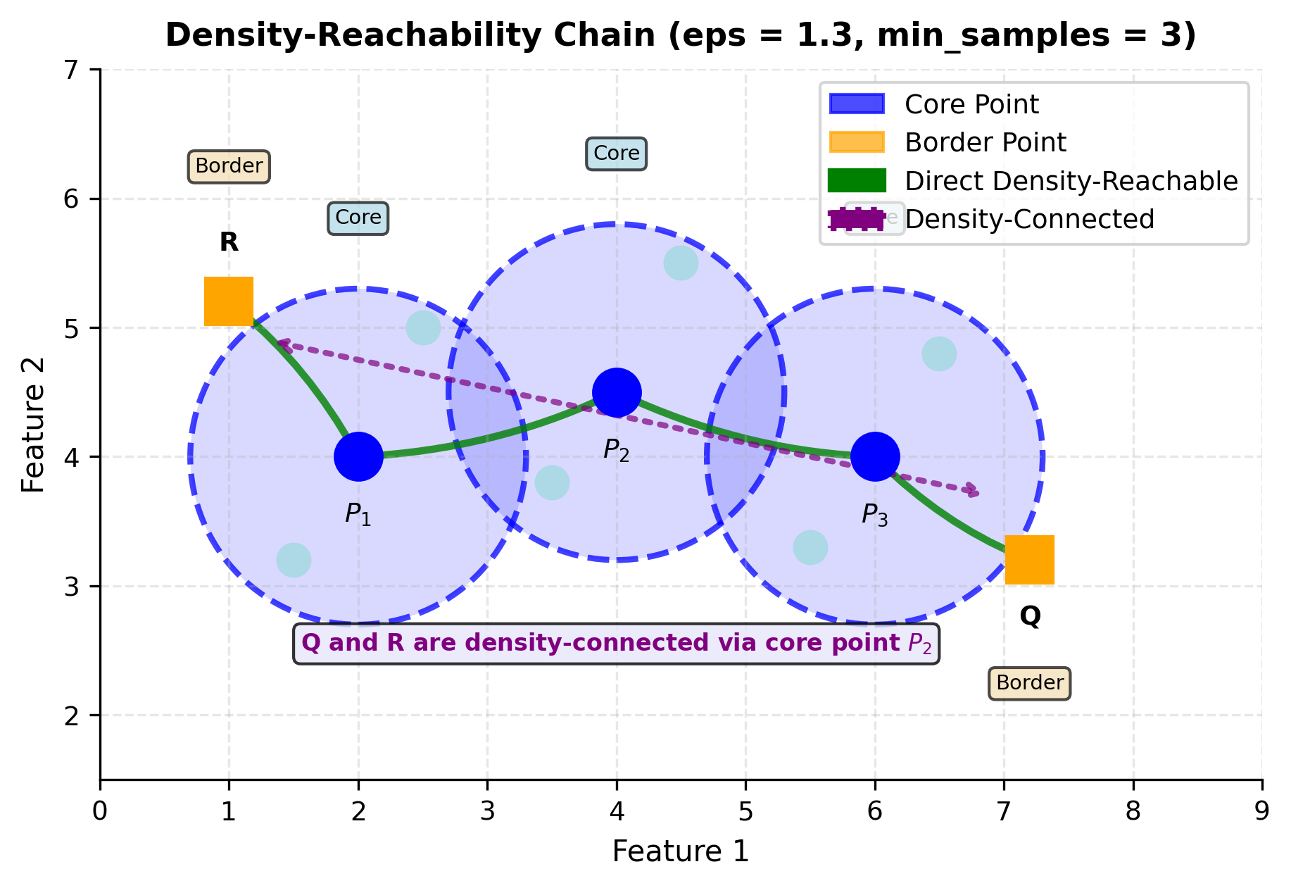
The green arrows show direct density-reachability: point is directly density-reachable from core point if and . The chain shows how core points can be mutually reachable, creating a "path" through dense regions.
The purple dashed line illustrates density-connectivity: points Q and R are density-connected because both are density-reachable from (Q through , R through ). This transitive relationship is what allows DBSCAN to form elongated clusters. Points don't need to be directly reachable from each other; they just need a common anchor from which both are reachable. This is the mathematical mechanism that enables DBSCAN to discover moon shapes, spirals, and other non-convex geometries.
The Complete Cluster Definition
We now have all the pieces of our neighborhood discovery system:
- Proximity circles that define local neighborhoods
- Density thresholds that identify crowded areas
- Reachability chains that connect dense regions
- Connectivity relationships that ensure symmetric belonging
The final step is defining what makes a valid cluster, a complete neighborhood that deserves its own distinct identity. A cluster in DBSCAN must satisfy two essential properties:
Property 1: Maximality. If a point belongs to the cluster, then every point reachable from it through dense pathways must also belong:
Let's parse this carefully:
- means "for all points and ". We're making a universal claim about every pair of points.
- means point is a member of cluster .
- is the logical AND: we're considering cases where is in AND is reachable from .
- is logical implication: "if... then..." In this case, if is in the cluster and is reachable from , then must also be in the cluster.
This property provides the completeness guarantee: a neighborhood can't have "missing members" who should logically be included based on density connections.
Property 2: Connectivity. Every pair of points in the cluster must be linked through the same dense network:
This says: for every pair of points both in cluster , those points must be density-connected (sharing some common anchor). This provides the unity principle: all members share a common origin in the dense activity network.
Maximality prevents incomplete neighborhoods (ensuring we don't leave out points that should belong), while connectivity prevents artificial mergers (ensuring we don't combine communities that should remain separate). Together, these properties ensure each cluster is both fully populated and genuinely unified.
What about the leftover points? They become noise: points that fall outside all dense networks, living in the sparse spaces between communities. This honest treatment of outliers, rather than forcing them into artificial clusters, is one of DBSCAN's greatest strengths.
Summary: The Complete Mathematical Framework
We've constructed a comprehensive system for discovering clusters of any shape by following the natural flow of density through data:
| Concept | Formula | What It Does |
|---|---|---|
| ε-Neighborhood | Defines "nearby" for each point | |
| Core Point | Identifies dense regions | |
| Direct Density-Reachable | is core | Single-step connections from dense areas |
| Density-Reachable | Chain: | Multi-step paths through core points |
| Density-Connected | reachable from | Symmetric cluster membership |
| Cluster | Maximal + Connected set | Complete, unified neighborhood |
Each definition builds on the previous ones, transforming our intuitive city-walking metaphor into rigorous, executable mathematics.
From Mathematics to Algorithm
Our mathematical framework is elegant and complete, but mathematical beauty alone doesn't find clusters in data. Now we must translate these concepts into a systematic procedure. The DBSCAN algorithm transforms our density-based intuition into concrete, executable steps.
The algorithm operates in three coordinated phases:
Phase 1: Preparation. Before exploring, we set up our data structures:
- Initialize all points as "unvisited"
- Create an empty cluster label array (all points start unlabeled)
- Set cluster counter to 0
- Define parameters: eps (neighborhood radius) and min_samples (density threshold)
Phase 2: Systematic Survey. For every unvisited point in the dataset, we ask: "Could this be the heart of a new neighborhood?"
For each unvisited point p:
    1. Mark p as visited
    2. Find N_eps(p) = all points within eps distance of p
    3. If |N_eps(p)| < min_samples:
         Mark p as NOISE (tentatively)
    4. Else:
         Increment cluster counter
         Expand cluster from p (Phase 3)
The key insight is that noise classification is tentative. A point initially marked as noise might later be absorbed into a cluster if it falls within the eps-neighborhood of a subsequently discovered core point.
Phase 3: Cluster Expansion. When we discover a core point, we expand outward following density-reachability chains:
ExpandCluster(p, neighbors, cluster_id):
    1. Add p to cluster cluster_id
    2. Create queue Q = neighbors
    3. While Q is not empty:
         a. Remove point q from Q
         b. If q is unvisited:
              Mark q as visited
              Find N_eps(q)
              If |N_eps(q)| >= min_samples:
                   Add N_eps(q) to Q  (q is a core point)
         c. If q is not yet in any cluster:
              Add q to cluster cluster_id
This expansion procedure implements our maximality property: we keep growing the cluster until we've absorbed every density-reachable point.
Each core point we discover acts like a seed that sends out explorers to map connected territory. This creates expanding waves of neighborhood discovery, ensuring no community member gets left behind. Border points get absorbed but don't propagate the expansion further.
The procedure directly implements our mathematical definitions. By following density-reachability chains, we ensure each cluster is both maximally complete (includes all density-reachable points) and genuinely cohesive (all members are density-connected).
Computational Complexity
The basic DBSCAN algorithm has time complexity in the worst case, where is the number of data points. This occurs when every point needs to be compared with every other point. However, with spatial indexing structures like R-trees or k-d trees, the complexity can be reduced to for low-dimensional data.
DBSCAN requires space to store the dataset and maintain neighborhood information. The algorithm doesn't need to store distance matrices or other quadratic space structures, making it memory-efficient compared to some other clustering algorithms.
Visualizing DBSCAN
Let's create visualizations that demonstrate how DBSCAN works with different types of data and parameter settings. We'll show the algorithm's ability to find clusters of arbitrary shapes and handle noise effectively.
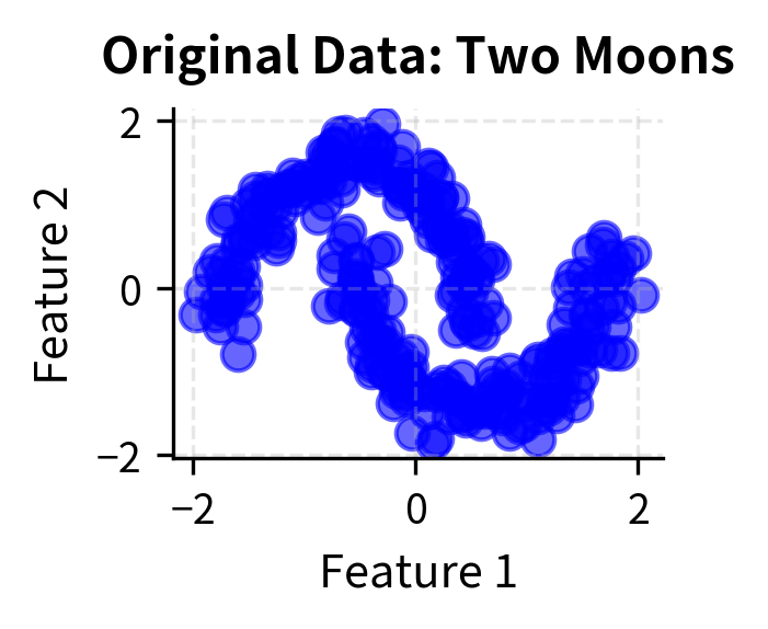
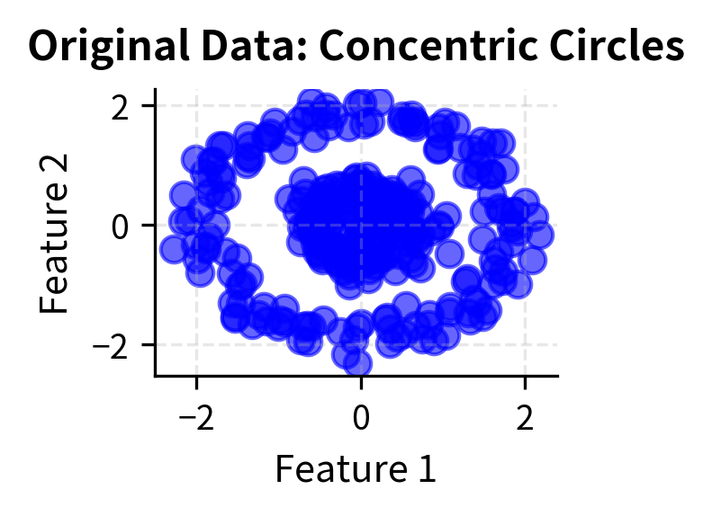
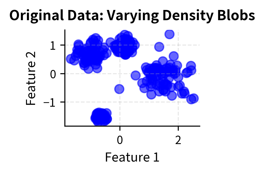
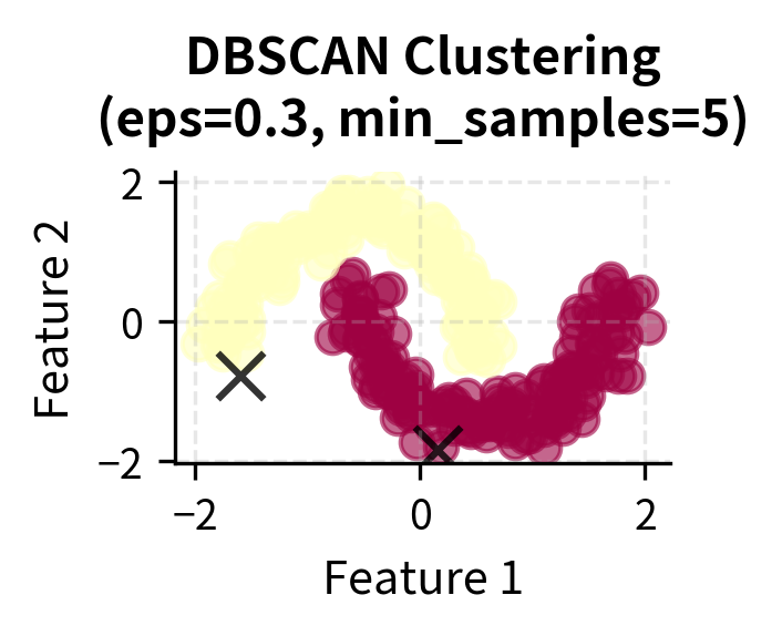
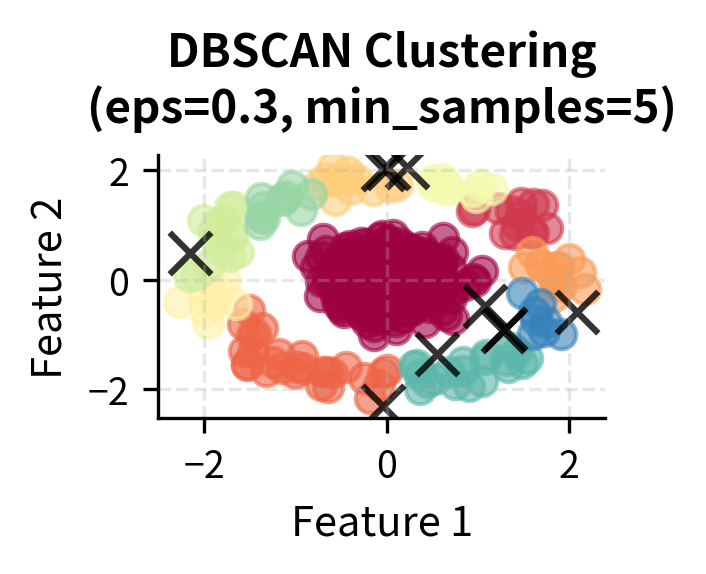
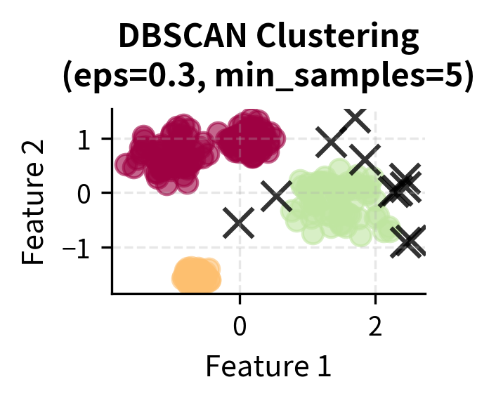
Here you can see DBSCAN's key strengths in action: it can identify clusters of arbitrary shapes (moons, circles) and handle varying densities while automatically detecting noise points (shown in black with 'x' markers). The algorithm successfully separates the two moon-shaped clusters, identifies the concentric circular patterns, and finds clusters with different densities in the blob dataset.
Worked Example
Let's work through a concrete numerical example to see how DBSCAN's mathematical concepts translate into actual clustering decisions. We'll use a small dataset where we can trace every calculation by hand, building intuition for how the algorithm discovers clusters.
The Dataset
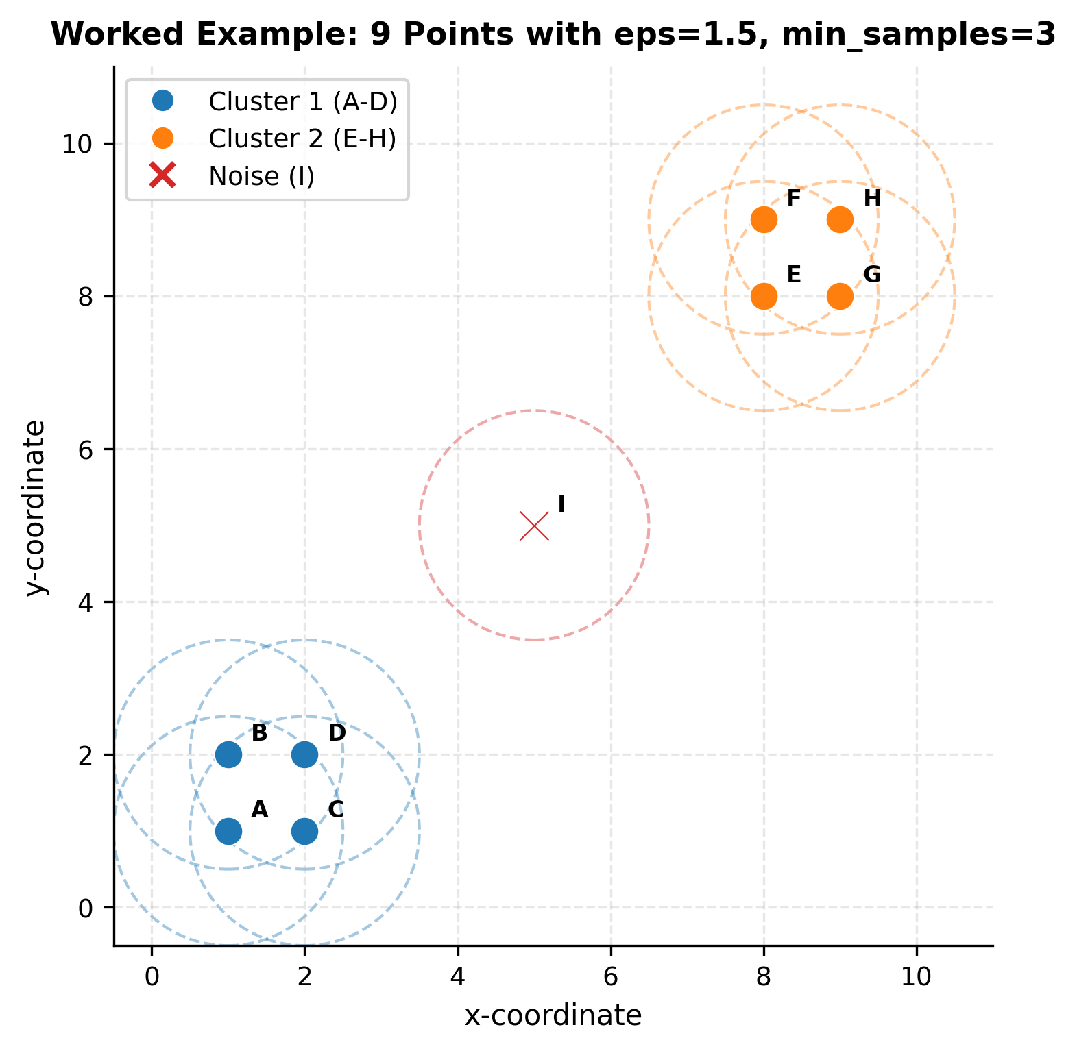
Consider nine points in 2D space, arranged to form two distinct groups with one isolated point:
| Point | Coordinates | Visual Location |
|---|---|---|
| A | (1, 1) | Lower-left cluster |
| B | (1, 2) | Lower-left cluster |
| C | (2, 1) | Lower-left cluster |
| D | (2, 2) | Lower-left cluster |
| E | (8, 8) | Upper-right cluster |
| F | (8, 9) | Upper-right cluster |
| G | (9, 8) | Upper-right cluster |
| H | (9, 9) | Upper-right cluster |
| I | (5, 5) | Isolated in center |
We'll use parameters: eps = 1.5 and min_samples = 3
Step 1: Calculate Distances
First, we need to find which points are neighbors. Using Euclidean distance:
Let's calculate key distances for point A:
- ✓ (within eps)
- ✓ (within eps)
- ✓ (within eps)
- ✗ (too far)
- ✗ (too far)
Since the lower-left and upper-right clusters are symmetric, similar calculations apply.
Step 2: Build Neighborhoods
For each point, we identify all neighbors within eps = 1.5:
| Point | Neighborhood | Size |
|---|---|---|
| A | {A, B, C, D} | 4 |
| B | {A, B, C, D} | 4 |
| C | {A, B, C, D} | 4 |
| D | {A, B, C, D} | 4 |
| E | {E, F, G, H} | 4 |
| F | {E, F, G, H} | 4 |
| G | {E, F, G, H} | 4 |
| H | {E, F, G, H} | 4 |
| I | {I} | 1 |
Notice that points A, B, C, D form a tightly connected group where everyone is neighbors with everyone else. The same is true for E, F, G, H. Point I stands alone.
Step 3: Identify Core Points
Now we apply the density test:
With min_samples = 3:
| Point | Neighborhood Size | ≥ 3? | Classification |
|---|---|---|---|
| A | 4 | ✓ | Core point |
| B | 4 | ✓ | Core point |
| C | 4 | ✓ | Core point |
| D | 4 | ✓ | Core point |
| E | 4 | ✓ | Core point |
| F | 4 | ✓ | Core point |
| G | 4 | ✓ | Core point |
| H | 4 | ✓ | Core point |
| I | 1 | ✗ | Not core |
All points in the two dense groups qualify as core points. Point I, with only itself in its neighborhood, fails the density test.
Step 4: Expand Clusters
Now we execute the DBSCAN algorithm, visiting points and expanding clusters:
Iteration 1: Visit point A
- Mark A as visited
- A is a core point → Create Cluster 1
- Add A to Cluster 1: {A}
- Queue A's neighbors for expansion: {B, C, D}
- Process B: visited, core point, add to Cluster 1, queue B's unvisited neighbors
- Process C: visited, core point, add to Cluster 1, queue C's unvisited neighbors
- Process D: visited, core point, add to Cluster 1
- Queue is empty → Cluster 1 complete: {A, B, C, D}
Iteration 2: Visit point E (first unvisited point)
- Mark E as visited
- E is a core point → Create Cluster 2
- Add E to Cluster 2: {E}
- Queue E's neighbors for expansion: {F, G, H}
- Process F, G, H similarly
- Cluster 2 complete: {E, F, G, H}
Iteration 3: Visit point I (last unvisited point)
- Mark I as visited
- I is NOT a core point (only 1 neighbor)
- I is not in any core point's neighborhood
- Mark I as noise
Final Result
| Cluster | Members | Description |
|---|---|---|
| Cluster 1 | {A, B, C, D} | Lower-left dense region |
| Cluster 2 | {E, F, G, H} | Upper-right dense region |
| Noise | {I} | Isolated point |
DBSCAN successfully identified two distinct clusters based on density while correctly classifying the isolated point I as noise. The algorithm never required us to specify the number of clusters; it discovered them naturally by following density connections.
Notice that every point in both clusters is a core point. In more complex scenarios, clusters often contain a mix of core points (in dense interiors) and border points (on cluster edges). Border points are reachable from core points but don't have enough neighbors themselves to be core points.
Implementation in Scikit-learn
Scikit-learn provides a robust and efficient implementation of DBSCAN that handles the complex neighborhood calculations and cluster expansion automatically. Let's explore how to use it effectively with proper parameter tuning and result interpretation.
Step 1: Data Preparation
First, we'll create a dataset with known cluster structure and some noise points to demonstrate DBSCAN's capabilities:
The dataset contains 550 points with 4 true clusters and 50 noise points. Standardization is crucial for DBSCAN because the algorithm relies on distance calculations, and features with different scales would dominate the clustering process.
Step 2: Parameter Tuning
Choosing appropriate values for eps and min_samples is crucial for DBSCAN's success. One systematic approach is to use the k-distance graph to find a suitable eps value. This method plots the distance to the k-th nearest neighbor for each point (where k = min_samples - 1) and looks for an "elbow" in the curve.
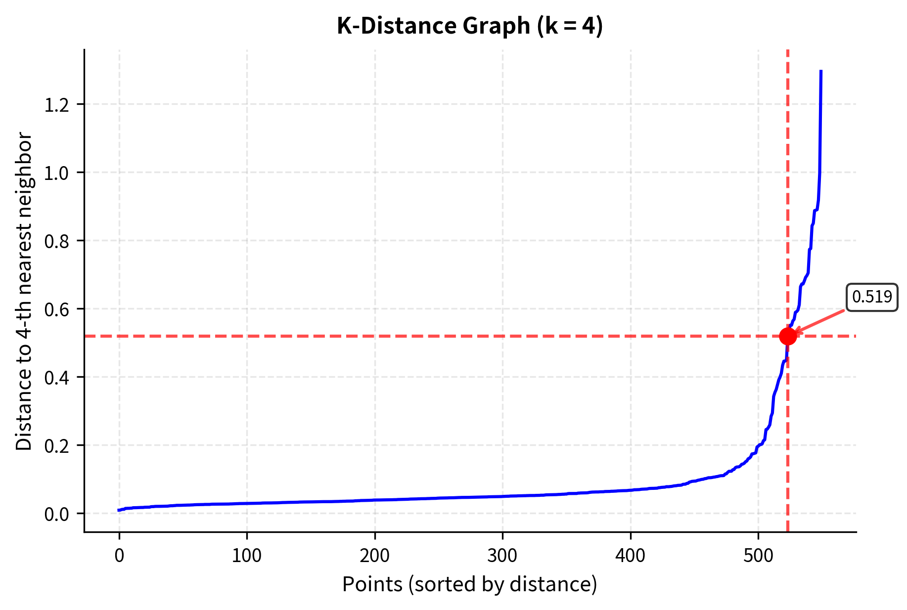
The k-distance graph reveals the data's density structure. The "elbow" point (around distance 0.5) indicates where dense regions transition to sparse regions, suggesting an optimal eps value. Points with smaller k-distances are in dense areas, while those with larger distances are in sparser regions.
Another useful perspective is the distribution of nearest neighbor distances across all points, which shows the overall density structure of the data:
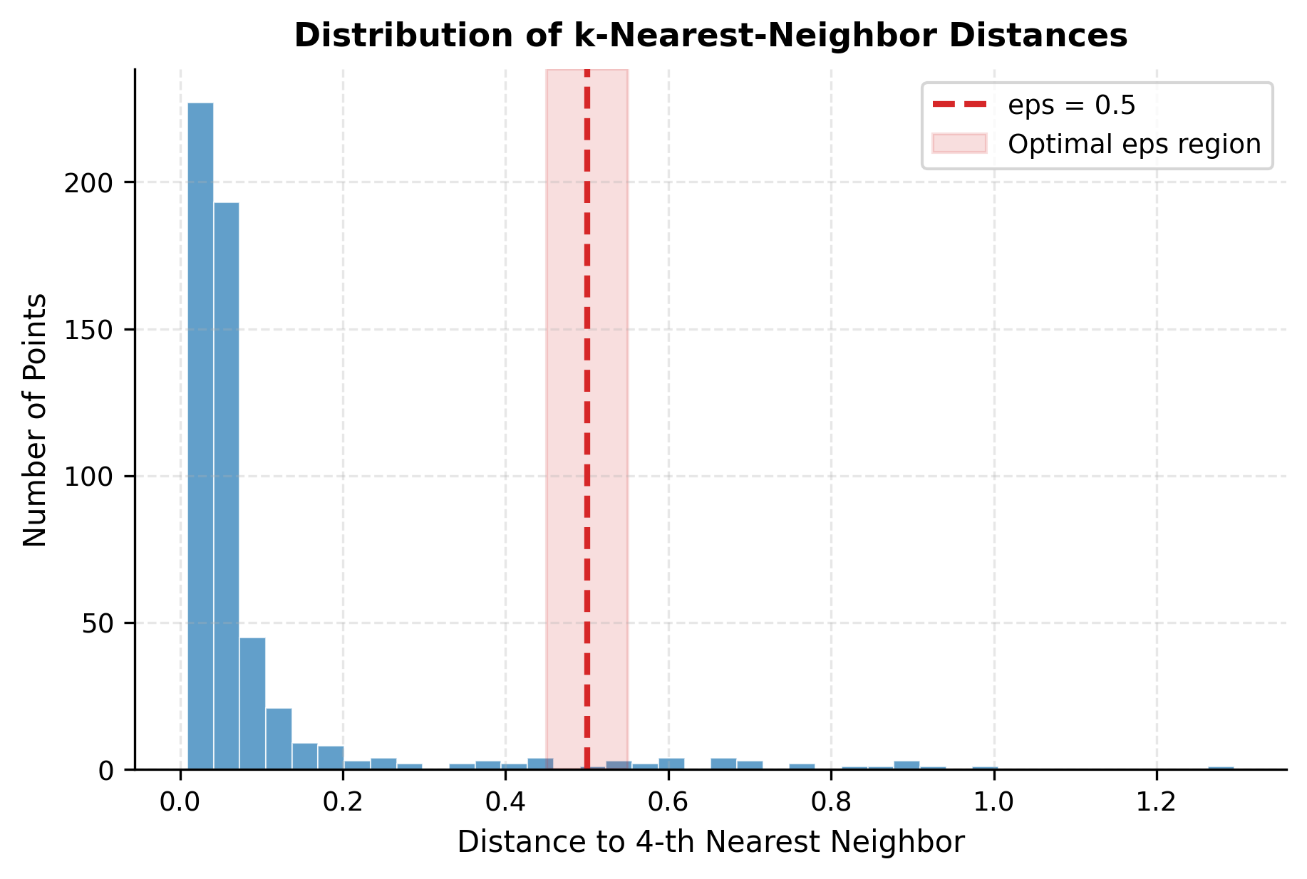
The histogram's bimodal structure is revealing: the left peak represents points in dense cluster cores with many nearby neighbors, while the right tail represents points in sparse regions, at cluster boundaries, or noise. Choosing eps in the transition zone captures the natural density structure.
Now let's systematically explore how different parameter combinations affect clustering results. The heatmap below shows the number of clusters discovered for a grid of eps and min_samples values:
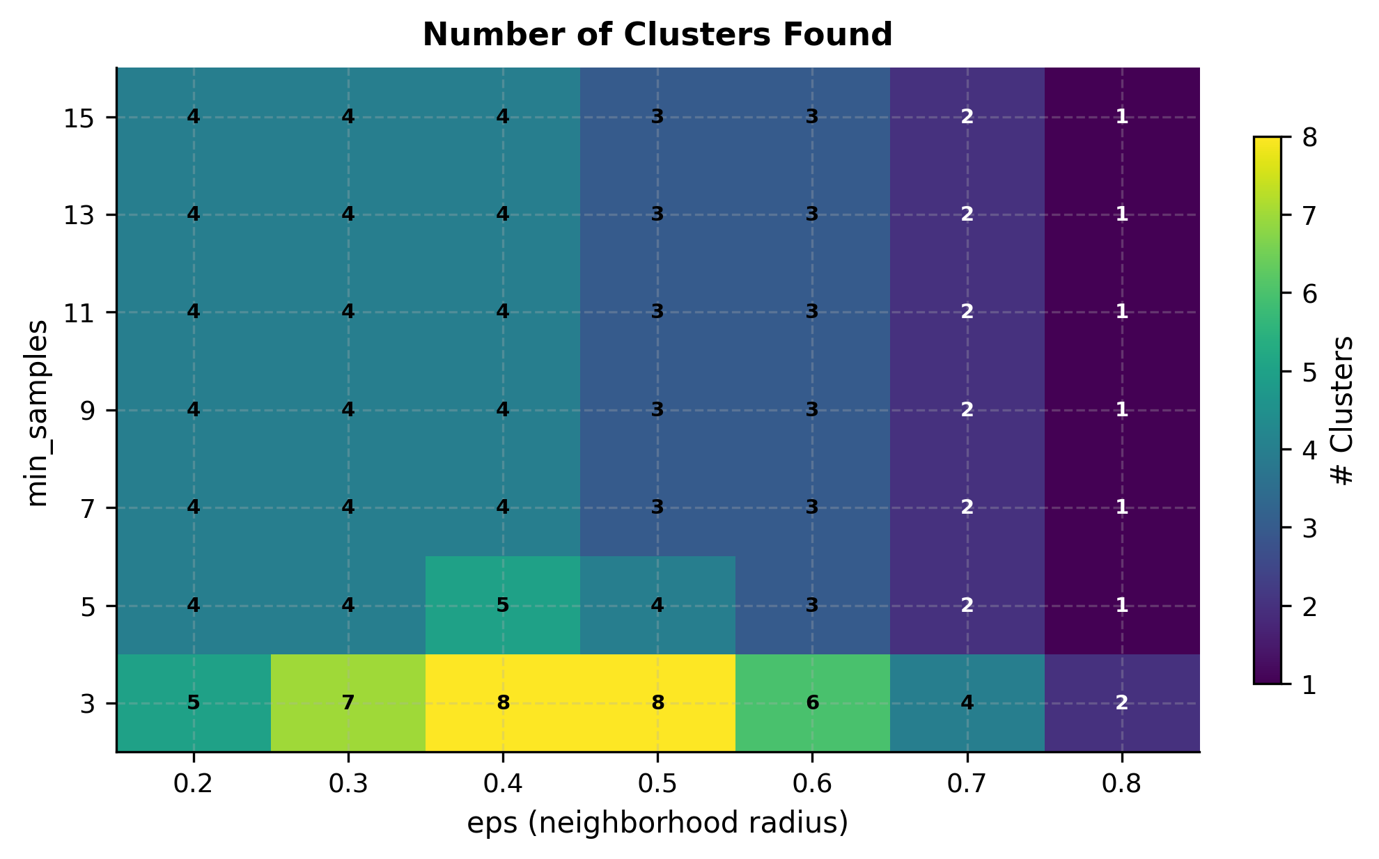
The heatmap reveals the interplay between parameters. With low eps and high min_samples, DBSCAN finds few or no clusters because density requirements are too strict. With high eps and low min_samples, distinct clusters may merge. The region around eps=0.5 and min_samples=5 correctly identifies 4 clusters for this dataset.
Now let's test specific parameter combinations to understand their impact on clustering results:
Step 3: Model Evaluation and Visualization
Based on the parameter comparison results, we'll use the best performing configuration and visualize the results:
The results show that DBSCAN successfully identified the correct number of clusters and properly classified noise points. The Adjusted Rand Index of approximately 0.85 indicates good agreement with the true cluster structure.
Step 4: Visualization
Let's create a comparison between the true clusters and DBSCAN results:
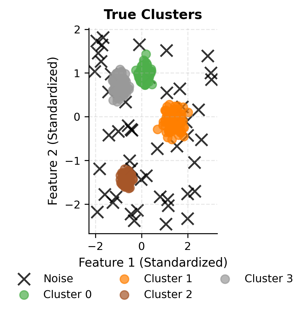
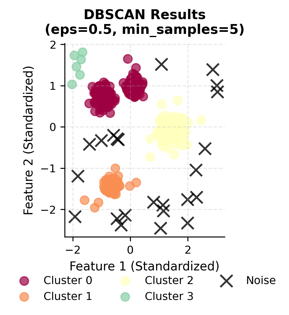
You can clearly see how DBSCAN successfully identifies the four main clusters while correctly classifying noise points. Let's examine the cluster size distribution to understand how DBSCAN handles varying densities:
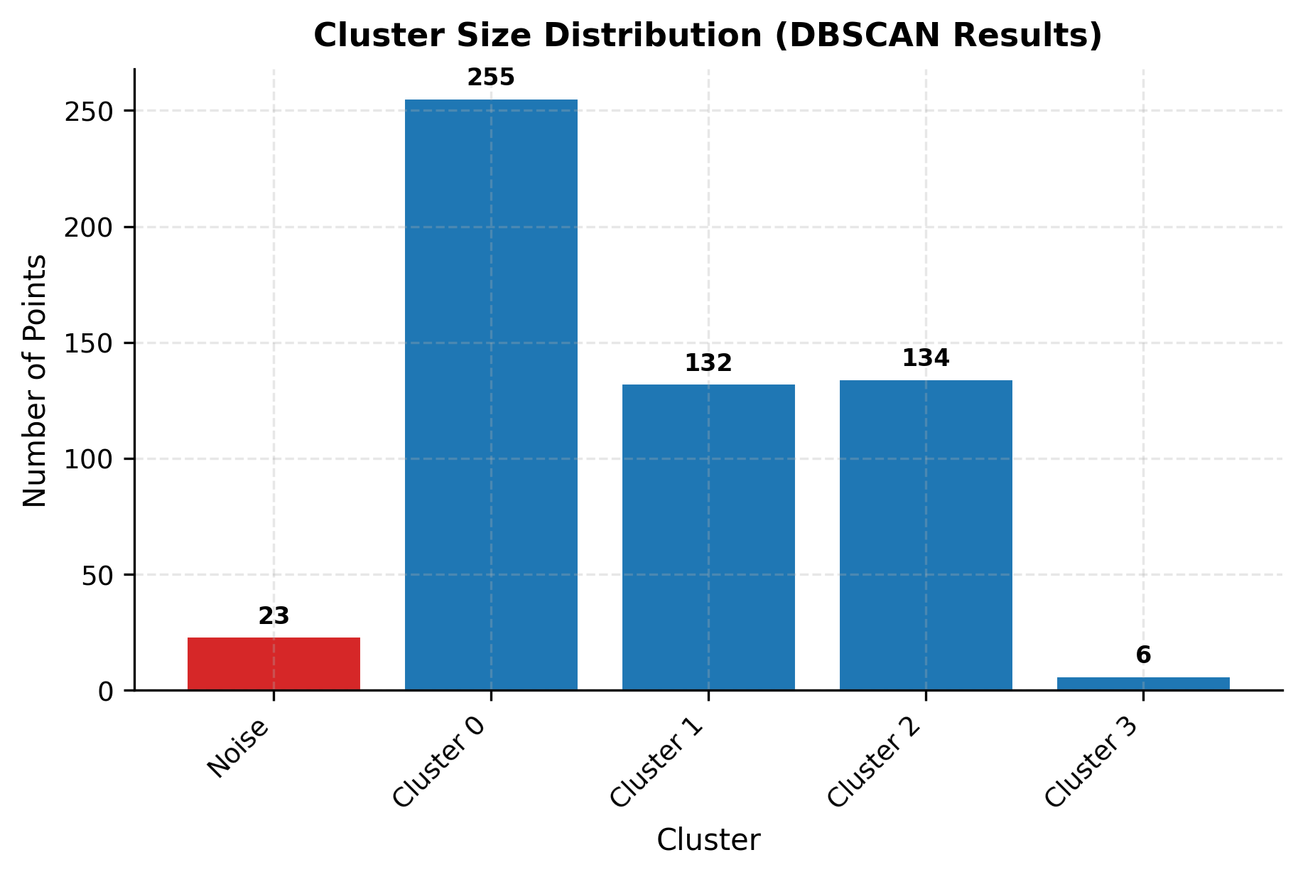
The cluster sizes vary significantly, reflecting the different standard deviations used when generating the synthetic data. DBSCAN successfully discovered all four clusters despite their different densities, and correctly classified approximately 50+ points as noise, close to the 50 noise points injected into the dataset.
Key Parameters
Below are some of the main parameters that affect how DBSCAN works and performs.
-
eps: The maximum distance between two samples for one to be considered in the neighborhood of the other. Smaller values create more restrictive neighborhoods, leading to more clusters and more noise points. Larger values allow more points to be connected, potentially merging distinct clusters. -
min_samples: The minimum number of samples in a neighborhood for a point to be considered a core point. Higher values require more dense regions to form clusters, leading to fewer clusters and more noise points. Lower values allow clusters to form in less dense regions. -
metric: The distance metric to use when calculating distances between points. Default is 'euclidean', but other options include 'manhattan', 'cosine', or custom distance functions. -
algorithm: The algorithm to use for nearest neighbor searches. 'auto' automatically chooses between 'ball_tree', 'kd_tree', and 'brute' based on the data characteristics.
Key Methods
The following are the most commonly used methods for interacting with DBSCAN.
-
fit(X): Fits the DBSCAN clustering algorithm to the data X. This method performs the actual clustering and stores the results in the object. -
fit_predict(X): Fits the algorithm to the data and returns cluster labels. This is the most commonly used method as it combines fitting and prediction in one step. -
predict(X): Predicts cluster labels for new data points based on the fitted model. For new points, it assigns them to existing clusters if they are within eps distance of a core point, or labels them as noise (-1) otherwise. -
core_sample_indices_: Returns the indices of core samples found during fitting. These are the points that have at least min_samples neighbors within eps distance. -
components_: Returns the core samples themselves (the actual data points that are core samples).
Practical Implications
DBSCAN is particularly valuable in several practical scenarios where traditional clustering methods fall short. In spatial data analysis, DBSCAN excels because geographic clusters often have irregular shapes that follow natural boundaries like coastlines, city limits, or street patterns. The algorithm can identify crime hotspots that follow neighborhood boundaries rather than forcing them into circular shapes, making it effective for urban planning and public safety applications.
The algorithm is also effective in image segmentation and computer vision applications, where the goal is to group pixels with similar characteristics while automatically identifying and removing noise or artifacts. DBSCAN can segment images based on color, texture, or other features, creating regions that follow the natural contours of objects in the image. This makes it valuable for medical imaging, satellite imagery analysis, and quality control in manufacturing.
In anomaly detection and fraud detection, DBSCAN's built-in noise detection capabilities make it suitable for identifying unusual patterns while treating normal observations as noise. The algorithm can detect fraudulent transactions, unusual network behavior, or outliers in sensor data without requiring separate anomaly detection methods. This natural integration of clustering and noise detection makes DBSCAN valuable in cybersecurity, financial services, and quality control applications.
Best Practices
To achieve optimal results with DBSCAN, start by standardizing your data using StandardScaler or MinMaxScaler, as the algorithm relies on distance calculations where features with larger scales will disproportionately influence results. Use the k-distance graph to determine an appropriate eps value by plotting the distance to the k-th nearest neighbor for each point and looking for an "elbow" in the curve. This visualization helps identify a natural threshold where the distance increases sharply, indicating a good separation between dense regions and noise.
When selecting min_samples, consider your dataset size and desired cluster tightness. A common heuristic is to set min_samples to at least the number of dimensions plus one, though this should be adjusted based on domain knowledge. Start with conservative values and experiment systematically. Evaluate clustering quality using multiple metrics including silhouette score, visual inspection, and domain-specific validation rather than relying on any single measure.
Data Requirements and Pre-processing
DBSCAN works with numerical features and requires careful preprocessing for optimal performance. Handle missing values through imputation strategies appropriate to your domain, such as mean/median imputation for continuous variables or mode imputation for categorical ones. Categorical variables must be encoded numerically using one-hot encoding for nominal categories or ordinal encoding for ordered categories, keeping in mind that the encoding choice affects distance calculations.
The algorithm performs best on datasets with sufficient density, typically requiring at least several hundred points to form meaningful clusters. For high-dimensional data (more than 10-15 features), consider dimensionality reduction techniques like PCA or feature selection before clustering, as distance metrics become less meaningful in high-dimensional spaces. The curse of dimensionality can cause all points to appear equidistant, undermining DBSCAN's density-based approach.
Common Pitfalls
A frequent mistake is using a single eps value when the dataset contains clusters with varying densities. DBSCAN uses global parameters that apply uniformly across the entire dataset, so if one region has much higher density than another, the algorithm may either miss sparse clusters (if eps is too small) or merge distinct dense clusters (if eps is too large). Consider using HDBSCAN as an alternative when dealing with varying density clusters.
Another pitfall is not accounting for the curse of dimensionality. In high-dimensional spaces, distance metrics lose their discriminative power, making it harder for DBSCAN to distinguish between dense and sparse regions effectively.
Over-interpreting clustering results is also problematic. DBSCAN will identify patterns even in random data, so validate results using domain knowledge, multiple evaluation metrics, and visual inspection. Check whether the identified clusters align with known categories or business logic rather than accepting the mathematical output at face value.
Computational Considerations
DBSCAN has a time complexity of for optimized implementations, but can be for brute-force approaches. For large datasets (typically >100,000 points), consider using approximate nearest neighbor methods or sampling strategies to make the algorithm computationally feasible. The algorithm's memory requirements can also be substantial for large datasets due to the need to store distance information.
Consider using more efficient implementations or approximate DBSCAN methods for large datasets. For very large datasets, consider using Mini-Batch K-means or other scalable clustering methods as alternatives, or use DBSCAN on a representative sample of the data.
Performance and Deployment Considerations
Evaluating DBSCAN performance requires careful consideration of both the clustering quality and the noise detection capabilities. Use metrics such as silhouette analysis to evaluate cluster quality, and consider the proportion of noise points as an indicator of the algorithm's effectiveness. The algorithm's ability to handle noise and identify clusters of arbitrary shapes makes it particularly valuable for exploratory data analysis.
Deployment considerations for DBSCAN include its computational complexity and parameter sensitivity, which require careful tuning for optimal performance. The algorithm is well-suited for applications where noise detection is important and when clusters may have irregular shapes. In production, consider using DBSCAN for initial data exploration and then applying more scalable methods for large-scale clustering tasks.
Summary
DBSCAN represents a fundamental shift from centroid-based clustering approaches by focusing on density rather than distance to cluster centers. This density-based perspective allows the algorithm to discover clusters of arbitrary shapes, automatically determine the number of clusters, and handle noise effectively - capabilities that make it invaluable for exploratory data analysis and real-world applications where data doesn't conform to simple geometric patterns.
The algorithm's mathematical foundation, built on the concepts of density-reachability and density-connectivity, provides a robust framework for understanding how points can be grouped based on their local neighborhood characteristics. While the parameter sensitivity and computational complexity present challenges, the algorithm's flexibility and noise-handling capabilities make it a powerful tool in the data scientist's toolkit.
DBSCAN's practical value lies in its ability to reveal the natural structure of data without imposing artificial constraints about cluster shape or number. Whether analyzing spatial patterns, segmenting images, or detecting anomalies, DBSCAN provides insights that other clustering methods might miss, making it a valuable technique for understanding complex, real-world datasets.
Quiz
Ready to test your understanding of DBSCAN clustering? Take this quick quiz to reinforce what you've learned about density-based clustering algorithms.

Comments