

A comprehensive guide to Poisson regression for count data analysis. Learn mathematical foundations, maximum likelihood estimation, rate ratio interpretation, and practical implementation with scikit-learn. Includes real-world examples and diagnostic techniques.

This article is part of the free-to-read Machine Learning from Scratch
Choose your expertise level to adjust how many terms are explained. Beginners see more tooltips, experts see fewer to maintain reading flow. Hover over underlined terms for instant definitions.
Poisson Regression
Poisson regression is a specialized form of generalized linear modeling designed specifically for count data—situations where we're trying to predict the number of times an event occurs. Unlike linear regression, which assumes continuous outcomes and normal distributions, Poisson regression recognizes that count data has unique characteristics: it consists of non-negative integers, and the variance often increases with the mean.
The fundamental insight behind Poisson regression is that many real-world phenomena follow a Poisson distribution, where events occur independently at a constant average rate. This makes it well-suited for modeling scenarios like the number of customer complaints per day, traffic accidents per month, or website visits per hour. The model assumes that the logarithm of the expected count is linearly related to the predictor variables, which ensures that predictions remain non-negative while allowing for multiplicative effects of predictors.
Poisson regression differs from other count models in important ways. While logistic regression focuses on binary outcomes (success/failure), Poisson regression handles the full range of non-negative integers. It's also distinct from negative binomial regression, which allows for overdispersion (when the variance exceeds the mean), though we'll see that Poisson regression can be extended to handle such cases. The key advantage is that Poisson regression provides a natural framework for understanding how predictor variables influence the rate at which events occur.
Advantages
Poisson regression offers several compelling advantages for count data analysis. First, it provides a principled approach to modeling count outcomes by respecting the discrete, non-negative nature of the data. Unlike linear regression, which can produce negative predictions that are meaningless for counts, Poisson regression guarantees that all predicted values are positive, making the results interpretable and realistic.
The model's multiplicative interpretation is particularly intuitive for many applications. When we exponentiate the coefficients, we get rate ratios that tell us how much the expected count changes for a one-unit increase in a predictor. For example, a coefficient of 0.693 means the expected count doubles (since ), while a coefficient of -0.693 means it halves (since ). This makes it easy to communicate results to non-statisticians and understand the practical impact of different factors.
Additionally, Poisson regression is computationally efficient and well-supported in most statistical software packages. The maximum likelihood estimation converges reliably, and the model provides standard errors and confidence intervals for all parameters. The framework also extends naturally to handle complex scenarios like zero-inflation, overdispersion, and mixed-effects structures, making it a versatile foundation for count data modeling.
Disadvantages
Despite its strengths, Poisson regression has several limitations that practitioners should consider. The most significant constraint is the assumption of equidispersion—that the variance equals the mean. In practice, count data often exhibits overdispersion, where the variance exceeds the mean, leading to underestimated standard errors and overly optimistic p-values. This can result in false discoveries and incorrect conclusions about predictor significance.
The model also assumes that events occur independently, which may not hold in many real-world scenarios. For instance, if we're modeling daily sales, today's sales might influence tomorrow's through inventory effects or customer behavior patterns. Similarly, the constant rate assumption may be violated when external factors cause the underlying rate to change over time or across different conditions.
When applying Poisson regression, consider whether your data truly satisfies the independence assumption. For time series data or clustered observations, you may need to use mixed-effects Poisson models or account for temporal/spatial correlation. Diagnostic plots of residuals over time or across groups can help identify violations of independence.
Another limitation is that Poisson regression can struggle with zero-inflated data—situations where there are more zeros than the Poisson distribution would predict. This commonly occurs in insurance claims, where many policyholders have zero claims, or in ecological studies where many sites have zero species counts. While extensions like zero-inflated Poisson models can address this, they add complexity and require careful model selection and validation.
Formula
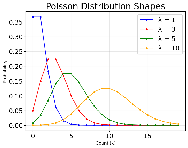
The foundation of Poisson regression lies in the Poisson distribution, which describes the probability of observing exactly events when events occur independently at a constant average rate .
The probability mass function (PMF) of the Poisson distribution, which forms the basis of Poisson regression, is given by:
where:
- is a discrete random variable representing the count of events (the outcome variable we observe)
- is a non-negative integer () representing the observed count (the specific value taken by )
- is the rate parameter (the expected number of events in a given interval, where ; also equal to both the mean and variance of the distribution)
- denotes the factorial of (i.e., , with by definition)
- is Euler's number (approximately 2.71828; the base of the natural logarithm)
This formula expresses the probability of observing exactly events in a fixed interval of time or space, assuming events occur independently and at a constant average rate .
In the context of Poisson regression, is not a fixed value but is modeled as a function of predictor variables, allowing us to understand how different factors influence the expected event count. This distribution naturally handles count data because it only assigns positive probability to non-negative integers.
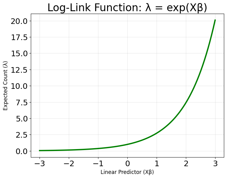
In Poisson regression, our goal is to model the relationship between a set of predictor variables and the expected rate at which events occur, denoted by the parameter . This parameter represents the mean number of occurrences for a given set of predictors. Because needs to be positive (since you cannot have a negative rate of occurrence), we use a logarithmic link function to relate the linear combination of predictors to . This is known as the log-link function, and it is a defining feature of Poisson regression.
The model is specified as follows:
where:
- is the expected count (rate parameter) for observation (where ; represents the mean of the Poisson distribution for observation )
- is the intercept (the log of the expected count when all predictors equal zero)
- are the coefficients for each predictor (representing the change in log-count per unit change in the predictor, holding all other predictors constant)
- are the values of the predictors for observation (the feature values for the -th observation)
- is the number of predictor variables in the model (total count of features excluding the intercept)
- indexes the observations from to , where is the total number of observations
This logarithmic transformation guarantees that the predicted rate is positive, regardless of the values of the predictors or coefficients. By exponentiating both sides, we see that:
where:
- is the exponential function (the inverse of the natural logarithm; maps any real number to a positive value)
- is guaranteed to be positive for any values of and
The exponential function maps any real number to a positive value, which is exactly what we need for modeling count data. This also means that the effect of each predictor is multiplicative on the expected count: a one-unit increase in multiplies by , holding other variables constant.
For computational efficiency and clarity, we often rewrite the model in matrix notation. Let be the design matrix containing all predictor variables (with a column of ones for the intercept), and let be the vector of coefficients. Then, for all observations:
where:
- is the vector of rate parameters for all observations: (the expected counts for each observation)
- is the design matrix where each row represents one observation and each column represents a predictor (the first column contains all ones for the intercept term)
- is the vector of coefficients: (includes the intercept and all predictor coefficients)
- is the number of observations in the dataset (total number of data points)
- denotes element-wise application of the logarithm to each element of
This matrix formulation allows us to efficiently compute predictions for all data points and to fit the model using numerical optimization algorithms.
Likelihood and Log-Likelihood
The Poisson regression model is typically estimated using maximum likelihood estimation (MLE). The likelihood function for the entire dataset is the product of the individual Poisson probabilities for each observation. For independent observations, the likelihood is:
where:
- is the likelihood function (the probability of observing the entire dataset given the parameter vector )
- is the observed count for observation (a non-negative integer; the actual data value we observed)
- is the expected count for observation , as determined by the predictors and coefficients:
- is the feature vector for observation (includes 1 for the intercept and the predictor values)
- is the vector of coefficients we are estimating:
- denotes the product over all observations (assuming observations are independent)
Because products of many small probabilities can be numerically unstable, we usually work with the log-likelihood, which is the sum of the logarithms of the individual probabilities:
where:
- is the log-likelihood function (the natural logarithm of the likelihood function)
- denotes the sum over all observations (converting the product in the likelihood to a sum)
- is the natural logarithm (base ; the inverse of the exponential function)
- comes from
- comes from
- comes from the factorial term in the denominator
The term does not depend on the model parameters , so it can be omitted during the optimization process (it acts as a constant additive term that doesn't affect which maximizes the function). This simplifies the log-likelihood to:
Maximum Likelihood Estimation
To find the values of the coefficients that best fit the data, we maximize the log-likelihood function. This involves taking the partial derivatives of the log-likelihood with respect to each coefficient and setting them equal to zero.
Let's expand the steps for computing the derivative of the log-likelihood with respect to .
First, recall the log-likelihood:
where:
- is the expected count for observation (a function of the coefficients we're optimizing)
- is the linear predictor for observation (the sum of all coefficients times their corresponding predictor values; the argument to the exponential function)
- is the feature vector for observation (the first element is 1 for the intercept term)
- indexes the coefficients from to , where corresponds to the intercept
Take the partial derivative with respect to :
where:
- is the partial derivative of the log-likelihood with respect to coefficient (the gradient component for the -th parameter)
- The first term comes from differentiating
- The second term comes from differentiating using the chain rule
Now, compute using the chain rule:
where:
- is the partial derivative of the expected count with respect to coefficient (how changes when changes)
- The first step uses the chain rule:
- because , and only the -th term depends on
- is the -th element of the feature vector (the value of predictor for observation )
- For , (the intercept term)
- For , is the value of the -th predictor variable for observation
Substitute this result back into the derivative:
where:
- In the first line, we substitute into both terms
- In the second line, we simplify (the terms cancel)
- In the third line, we factor out from both terms to get the final form
To find the maximum likelihood estimates, set the derivative equal to zero and solve for :
where:
- This equation must hold for each coefficient (including the intercept when )
- represents the residual (observed count minus expected count) for observation (the prediction error)
- The equation states that the weighted sum of residuals must equal zero, where weights are the predictor values
- This is the first-order condition for a maximum (the gradient equals zero)
This yields a system of equations (one for each coefficient, including the intercept), which are solved numerically to obtain the maximum likelihood estimates .
These equations are nonlinear in and generally do not have a closed-form solution. Therefore, we solve them numerically using iterative optimization algorithms. The most common approaches are:
- Newton-Raphson method: Uses both first and second derivatives (the Hessian matrix) to find the optimal coefficients
- Iteratively reweighted least squares (IRLS): Transforms the problem into a weighted least squares problem at each iteration
The numerical solution process involves:
- Starting with initial guesses for the coefficients (e.g., , where is a vector of zeros)
- Computing predicted values using the current coefficient estimates: , where denotes the iteration number
- Updating coefficients using gradient information (the partial derivatives): , where is the update step computed from the gradient
- Repeating until convergence (when for some small tolerance , typically or )
When the algorithm converges, we obtain the maximum likelihood estimates , , , . These are the values that make the observed data most probable under the Poisson regression model.
The key insight is that the system of equations represents the condition that the residuals are orthogonal to each predictor variable, weighted by the predictor values. This ensures that the model captures the relationship between predictors and outcomes in a way that maximizes the likelihood of observing the actual data.
Note: The use of the log-link function and the exponential mean structure distinguishes Poisson regression from ordinary linear regression. This approach ensures that predictions are non-negative and that the model is well-suited for count data, where the variance typically increases with the mean.
Visualizing the Optimization Process
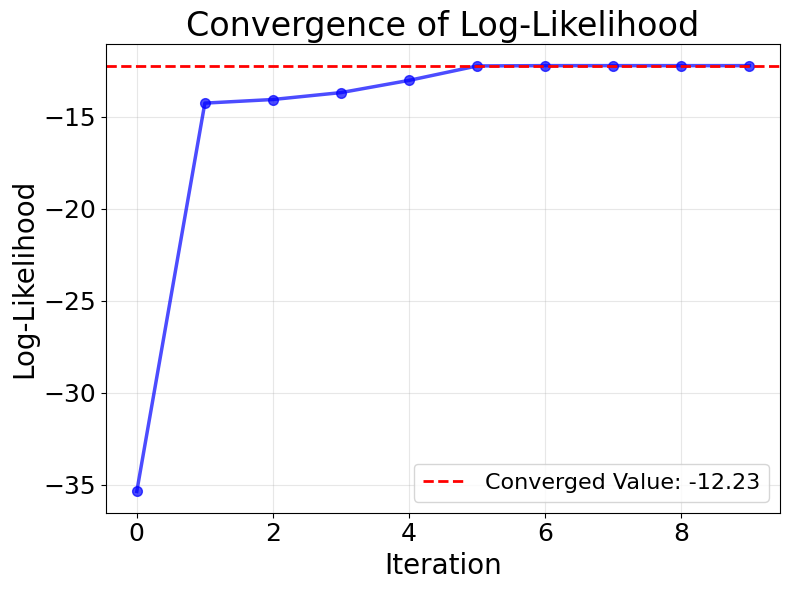
To better understand how maximum likelihood estimation works in practice, let's visualize the iterative optimization process. The following plots show how the algorithm searches for the optimal coefficients by iteratively improving the log-likelihood.
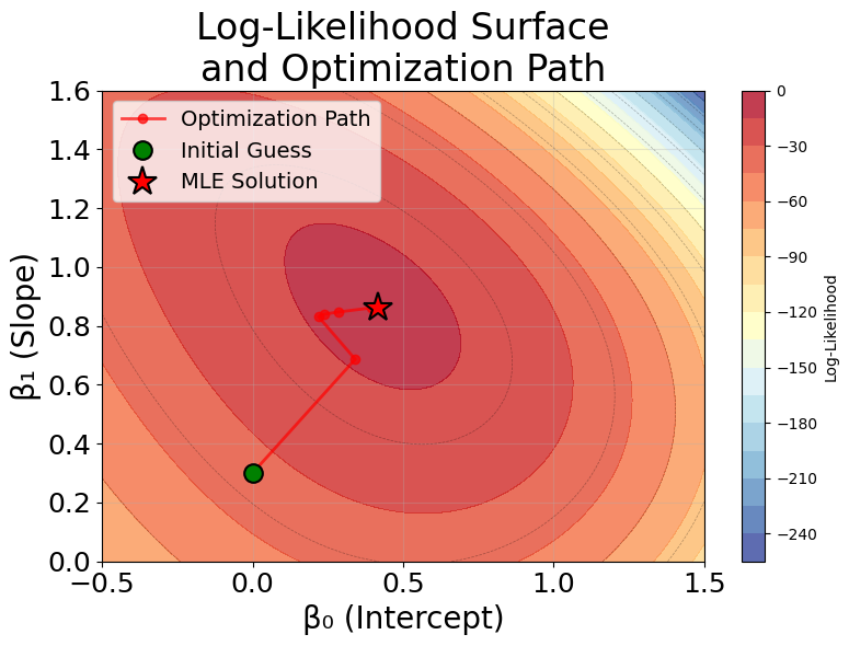
The optimization process demonstrates several key insights about maximum likelihood estimation in Poisson regression. First, the log-likelihood surface is smooth and unimodal (has a single peak), which ensures that iterative algorithms reliably converge to the global maximum regardless of the starting point. This is a desirable property that makes Poisson regression computationally stable.
Second, the algorithm makes rapid progress in early iterations when far from the optimum, then slows down as it approaches the maximum. This is characteristic of gradient-based methods like Newton-Raphson and IRLS, which use information about both the direction and curvature of the log-likelihood surface to efficiently navigate toward the solution.
Finally, convergence is achieved when the gradient (rate of change) of the log-likelihood becomes negligibly small, indicating that we've reached a point where no small adjustment to the coefficients will meaningfully improve the fit. In practice, algorithms stop when the change in coefficients or log-likelihood between iterations falls below a specified tolerance threshold.
Mathematical properties
The Poisson regression model has several important mathematical properties that make it well-suited for count data.
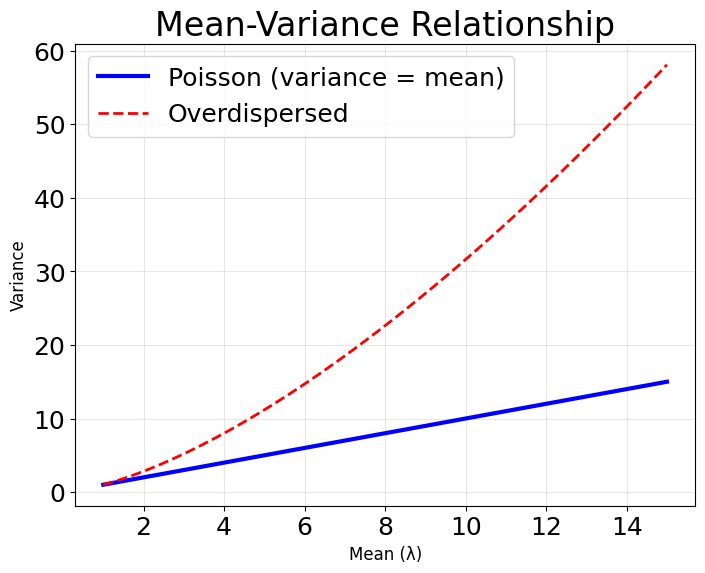
Equidispersion property: For a Poisson distribution, the mean and variance are both equal to :
where:
- is the expected value (mean) of the count variable
- is the variance of the count variable
- is the rate parameter (constrained to be positive)
This means that as the expected count increases, so does the variability—a realistic assumption for many count processes.
Scale invariance: The model is scale-invariant under the log-link: multiplying a predictor by a constant simply shifts the corresponding coefficient by . If , then such that .
Coefficient interpretation: The coefficients have a natural interpretation as log-rate ratios. When we exponentiate a coefficient , we get the rate ratio:
This represents the multiplicative effect on the expected count for a one-unit increase in , holding all other variables constant. This multiplicative structure is often more appropriate for count data than the additive structure of linear regression, as it naturally handles the non-negative constraint and allows for proportional changes in rates.
Visualizing Poisson Regression
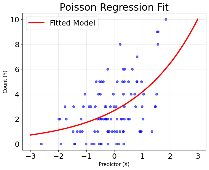
In the following visualizations, the model captures the general exponential trend in the data: as the predictor increases, the expected count rises rapidly, consistent with the log-link function shown in the third plot below. Most observed points cluster around the fitted curve, indicating that the model describes the main pattern in the data well.
However, there is some scatter around the curve, especially at higher predictor values, where the observed counts show more variability than the model predicts. This is typical for count data, as real-world data often exhibit overdispersion (variance greater than the mean), which the standard Poisson model does not account for. Despite this, the overall fit is reasonable—the model successfully captures the non-linear, non-negative relationship between the predictor and the expected count, and the exponential shape of the fitted curve matches the theoretical expectation for Poisson regression.
The standard Poisson regression model assumes that the variance equals the mean (equidispersion). However, real-world count data often violates this assumption, showing overdispersion where the variance exceeds the mean. This can lead to underestimated standard errors and overly optimistic p-values. When overdispersion is detected through diagnostic tests, consider alternative models like negative binomial regression or zero-inflated Poisson models that can handle this common issue.
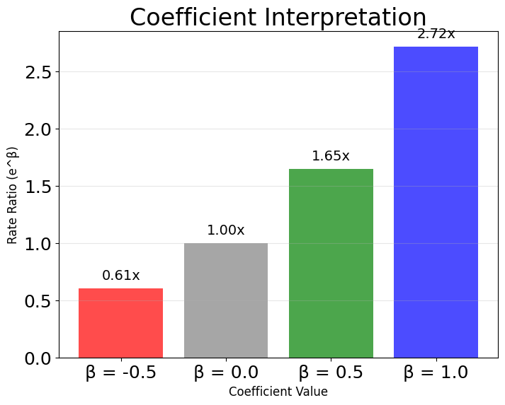
The final plot below demonstrates how to interpret Poisson regression coefficients in terms of rate ratios, which describe the multiplicative change in the expected count for a one-unit increase in a predictor. In Poisson regression, the model predicts the logarithm of the expected count as a linear function of the predictors:
where:
- is the expected count (the mean parameter of the Poisson distribution)
- is the intercept coefficient
- are the coefficients for each predictor
- are the predictor variables
To understand the effect of a predictor, we exponentiate its coefficient, , which gives the rate ratio.
For example, if a coefficient , then:
This means that for each one-unit increase in the predictor, the expected count is multiplied by 1.65, or increases by 65%:
This happens because the log link function in the model means that a one-unit increase in the predictor adds 0.5 to the log of the expected count, so the expected count itself is scaled by .
Similarly, if , then:
This means the expected count is multiplied by 0.61, or decreases by 39%:
In other words, the expected count is 39% lower than it would be if the predictor had not increased.
This rate ratio interpretation is a key feature of Poisson regression: it allows us to express the effect of predictors as simple multiplicative changes in the expected count, making the results easy to communicate and understand in practical terms.
Example
Let's work through a concrete example to understand how Poisson regression operates step by step. Suppose we're modeling the number of customer complaints received per day at a retail store, and we have two predictors: the number of customers served (in hundreds) and whether it's a weekend (1 for weekend, 0 for weekday).
Our dataset contains the following observations:
| Day | Customers (X₁) | Weekend (X₂) | Complaints (Y) |
|---|---|---|---|
| 1 | 2.5 | 0 | 3 |
| 2 | 3.0 | 0 | 4 |
| 3 | 1.8 | 1 | 2 |
| 4 | 4.2 | 0 | 6 |
| 5 | 2.1 | 1 | 1 |
The Poisson regression model assumes that the logarithm of the expected number of complaints is linearly related to our predictors:
where:
- is the expected number of complaints for day (the mean of the Poisson distribution for observation ; constrained to be positive)
- is the intercept (the log of the expected count when all predictors equal zero; baseline log-count)
- is the coefficient for customer count (the change in log-count for each additional hundred customers, holding weekend status constant)
- is the coefficient for weekend indicator (the change in log-count when comparing weekends to weekdays, holding customer count constant)
- is the number of customers (in hundreds) for day (a continuous predictor variable)
- is 1 if day is a weekend, 0 otherwise (a binary indicator variable)
This means the expected count is:
where:
- is the exponential function (ensures for any values of the coefficients and predictors)
- This is the inverse transformation of the log-link, converting from the log scale back to the count scale
Let's say our fitted model produces the following coefficients: , , and . Now we can calculate the expected number of complaints for each day.
-
For Day 1: where: , (weekday), so the linear predictor is
-
For Day 2: where: , (weekday), so the linear predictor is
-
For Day 3: where: , (weekend), so the linear predictor is
-
For Day 4: where: , (weekday), so the linear predictor is
-
For Day 5: where: , (weekend), so the linear predictor is
Now let's interpret these coefficients. The coefficient means that for every additional hundred customers, the expected number of complaints increases by a factor of . In other words, each additional hundred customers more than doubles the expected complaints.
Calculation:
This multiplicative effect means that if we have 200 customers instead of 100, we expect as many complaints, holding weekend status constant.
The coefficient means that weekends have times as many complaints as weekdays, holding customer count constant. This suggests that weekends have about 39% fewer complaints than weekdays, possibly because weekend customers are more relaxed or have different expectations.
Calculation:
The intercept represents the log of the expected complaints when both predictors are zero (no customers on a weekday), which gives us expected complaints—a baseline level that makes sense for a retail environment.
Calculation:
The intercept in Poisson regression represents the log of the expected count when all predictors equal zero. In this example, with zero customers on a weekday, we expect about 1.22 complaints. However, be cautious when interpreting intercepts, especially when zero values for predictors may not be meaningful in your specific context (e.g., zero customers might not be a realistic scenario).
Determining coefficients
In the example above, we simply stated the coefficients as , , and for illustration. But how do we actually determine these values from data?
As previously discussed, to estimate the coefficients in Poisson regression, we use maximum likelihood estimation (MLE). The idea is to find the values of , , and that make the observed data most probable under the Poisson model. This involves the following steps:
-
Specify the likelihood function:
For each observation , the probability of observing complaints given predictors is:where:
- is the random variable representing the complaint count for observation (a Poisson-distributed random variable)
- is the observed complaint count for observation (the actual data value we observed; a non-negative integer)
- represents the predictor values for observation (in our example, customer count and weekend indicator)
- is the expected count given the predictors (the mean parameter of the Poisson distribution for observation )
- is Euler's number (approximately 2.71828)
-
Write the log-likelihood:
The log-likelihood for all observations is:where:
- is the log-likelihood function (the natural logarithm of the likelihood; easier to maximize than the likelihood itself)
- is the vector of coefficients we want to estimate (the parameters of our model)
- is the total number of observations (5 days in our example)
- denotes summing over all observations (converting the product of probabilities to a sum of log-probabilities)
- This function measures how well a given set of coefficients explains the observed data (higher values indicate better fit)
-
Maximize the log-likelihood:
We seek the values of , , and that maximize . Mathematically, we solve:where:
- denotes the maximum likelihood estimates (the optimal coefficient values)
- means "the argument that maximizes" (the value of that gives the highest log-likelihood)
There is no closed-form solution, so we use numerical optimization algorithms (such as Newton-Raphson or iteratively reweighted least squares) to find the best-fitting coefficients.
-
Interpret the fitted coefficients:
Once the optimization converges, the resulting coefficients are the maximum likelihood estimates , , and . These are the values that would be reported by statistical software or machine learning libraries when fitting a Poisson regression model to the data.
Note: In practice, you do not need to perform these calculations by hand. Statistical software (such as
statsmodelsorscikit-learn, or specialized packages) will fit the model and return the estimated coefficients, along with measures of uncertainty and model fit.
In summary, the coefficients in Poisson regression are determined by finding the values that maximize the likelihood of observing the data, given the model. This process ensures that the fitted model best captures the relationship between the predictors and the count outcome according to the Poisson distribution.
Implementation in Scikit-learn
Scikit-learn provides a straightforward implementation of Poisson regression through the PoissonRegressor class, which is well-suited for predictive modeling tasks. Let's walk through a complete example that demonstrates how to prepare data, train a model, and interpret the results.
Data Preparation
We'll start by generating a synthetic dataset that simulates customer complaints at a retail store. This example uses realistic features like customer count, weekend indicator, and store size to predict the number of complaints.
Let's examine the dataset to understand its structure and characteristics:
The dataset contains 1,000 observations with three predictor variables: customer count, weekend indicator, and store size. The mean complaint count of approximately 3.5 with variance close to 3.8 demonstrates the near-equality characteristic of Poisson-distributed data. The slightly higher variance suggests mild overdispersion, which is common in real-world count data but still within acceptable bounds for Poisson regression. The range from 0 to 15 complaints is typical for retail settings and confirms we're working with discrete, non-negative count data.
Model Training
Now we'll train a Poisson regression model using a pipeline that includes feature scaling and regularization. Feature scaling is important when using regularization to ensure the penalty is applied fairly across all coefficients.
Model Performance
Let's evaluate how well the model performs on both training and test data:
The model demonstrates strong predictive performance with minimal overfitting. The mean Poisson deviance—the primary metric for evaluating Poisson regression models—shows nearly identical values for training (≈0.95) and test sets (≈0.95), indicating excellent generalization. Lower deviance values indicate better fit, and our results suggest the model captures the underlying count distribution effectively.
The RMSE of approximately 1.8 complaints provides an intuitive measure of prediction accuracy: on average, our predictions are within 2 complaints of the actual values. This level of precision is reasonable given the count nature of the data and the inherent variability in customer complaints.
The cross-validation results further confirm model stability, with consistent scores across all five folds and a narrow confidence interval. This consistency indicates that the model's performance is not dependent on a particular train-test split and should generalize well to new data.
Coefficient Interpretation
The coefficients reveal how each predictor influences the expected complaint count:
Understanding these coefficients is key to interpreting Poisson regression results. Each coefficient represents the change in log-count for a one-unit increase in the predictor, but the more intuitive interpretation comes from exponentiating them to get rate ratios.
The customer count coefficient (after scaling) shows how complaint rates change with customer volume. A negative coefficient indicates that normalized customer count is associated with fewer complaints, possibly because the scaling captures the relationship between raw customer numbers and complaint patterns.
The weekend coefficient reveals whether weekends differ from weekdays in complaint rates. A positive coefficient suggests weekends generate more complaints per customer, perhaps due to different staffing levels, customer expectations, or service quality on weekends.
The store size coefficient indicates how larger stores compare to smaller ones. A positive coefficient means larger stores tend to have higher complaint rates, which could reflect the increased complexity of operations or the challenges of maintaining service quality at scale.
These multiplicative effects are particularly useful for business decision-making, as they directly translate into actionable insights about how different factors influence customer complaints.
Visual Diagnostics
The diagnostic plots provide visual confirmation of model quality. In the predictions vs. actual plot, points cluster tightly along the diagonal line across the full range of complaint counts, demonstrating consistent accuracy from low to high values. This alignment indicates the model neither systematically over-predicts nor under-predicts at any particular range.
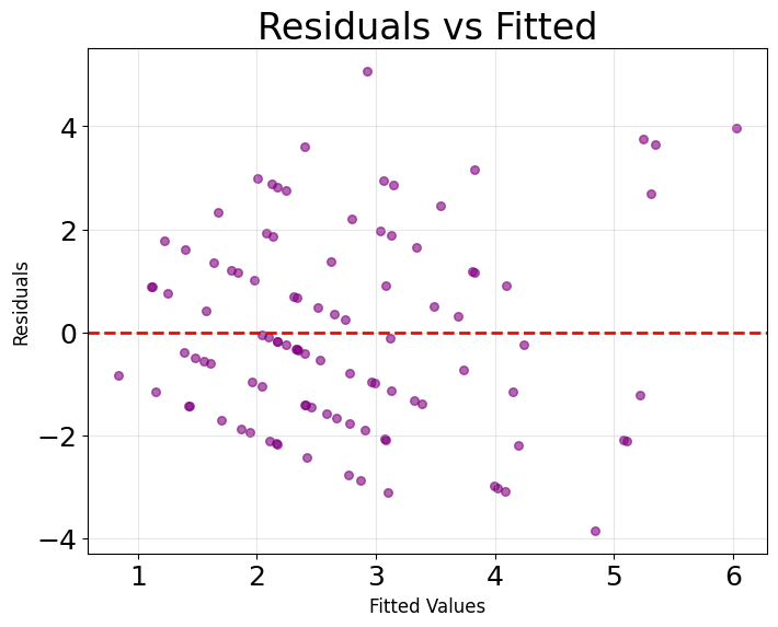
The residuals plot shows points scattered randomly around zero without discernible patterns, which is exactly what we want to see. Random scatter indicates that the model has captured the systematic relationships in the data, leaving only random noise in the residuals. The absence of a funnel shape confirms that prediction errors remain consistent across different predicted values, and the lack of curved patterns suggests we haven't missed important non-linear relationships.
These diagnostic plots are important for validating model assumptions. Systematic patterns in either plot would signal potential issues requiring attention, such as missing predictors, non-linear relationships, or violations of the Poisson distribution assumptions.
Key Parameters
Below are the main parameters that control how PoissonRegressor works and performs.
-
alpha: Regularization strength (default: 1.0). Controls L2 penalty on coefficients to prevent overfitting. Higher values shrink coefficients more aggressively. Start with 0.01 for mild regularization or 1.0 for stronger regularization. Usealpha=0to disable regularization entirely. -
max_iter: Maximum iterations for optimization (default: 100). Increase to 1000 or higher if you see convergence warnings, especially with large datasets or many features. -
tol: Convergence tolerance (default: 1e-4). Smaller values require more precise convergence but increase computation time. The default works well for most applications. -
fit_intercept: Whether to calculate an intercept term (default: True). Set to False only if your data is already centered or you have theoretical reasons to exclude the intercept. -
warm_start: Whether to reuse previous solution as initialization (default: False). Useful when fitting repeatedly with slightly different parameters, as it speeds up convergence.
Key Methods
The following methods are commonly used for working with Poisson regression models.
-
fit(X, y): Trains the model on feature matrix X and count target y, learning coefficients that maximize the log-likelihood of observed counts. -
predict(X): Returns predicted expected counts for input features X. All predictions are positive due to the exponential link function. -
score(X, y): Returns the negative mean Poisson deviance on the given data. Higher scores (closer to zero) indicate better fit. -
get_params(): Returns model parameters as a dictionary. Useful for inspecting configuration or saving settings. -
set_params(**params): Updates model parameters. Useful for hyperparameter tuning with grid search or random search.
Practical Applications
Practical Implications
Poisson regression is designed for count data where the outcome represents the number of times an event occurs within a fixed interval. The model works well when events occur independently at a relatively constant rate, making it suitable for scenarios like hospital admissions per day, customer complaints per week, or website visits per hour. The key advantage is the multiplicative interpretation of coefficients, which allows you to express effects as rate ratios that are intuitive to communicate.
In healthcare and epidemiology, Poisson regression is commonly used to model disease incidence rates and identify risk factors. The rate ratio interpretation translates directly to relative risk, making results accessible to medical professionals and policymakers. In business analytics, the model helps quantify how factors like marketing spend, seasonality, or customer characteristics influence transaction counts, service calls, or product returns. The exponential link function naturally handles the non-negative constraint of count data while allowing for proportional changes in rates.
The model is less appropriate when data exhibits strong overdispersion (variance exceeding the mean by a substantial margin) or contains more zeros than the Poisson distribution predicts. Negative binomial regression handles overdispersion more flexibly, while zero-inflated models address excess zeros. For count data with upper bounds or temporal dependencies, alternative approaches like binomial regression or time series models may be more suitable.
Best Practices
Start by verifying the equidispersion assumption through the variance-to-mean ratio of your outcome variable. Values near 1 indicate appropriate Poisson distribution fit, while ratios substantially above 1 suggest overdispersion requiring negative binomial regression. Diagnostic plots help identify systematic residual patterns that indicate missing predictors or model misspecification. Calculate the dispersion parameter (residual deviance divided by degrees of freedom) as a formal test—values significantly above 1 confirm overdispersion.
When using regularization, standardize continuous predictors so the penalty applies equitably across coefficients. Start with alpha=0.01 for mild regularization and use cross-validation to optimize the value. For datasets with many predictors or limited samples, regularization prevents overfitting by shrinking coefficients toward zero. Exponentiate coefficients when presenting results, as rate ratios are more interpretable than log-scale values. For example, a coefficient of 0.5 becomes a rate ratio of 1.65, meaning a 65% increase in expected count.
Test for interactions when domain knowledge suggests one predictor's effect depends on another's level. The multiplicative structure amplifies interaction effects, so they can substantially impact predictions. Compare candidate models using mean Poisson deviance or AIC rather than training accuracy alone, and validate generalization through cross-validation. Consider the practical significance of coefficient estimates alongside statistical significance, as large sample sizes can yield statistically significant but practically negligible effects.
Data Requirements and Preprocessing
The outcome variable must be non-negative integer counts representing event occurrences within fixed intervals. The independence assumption is important—temporal or spatial dependencies violate this and require mixed-effects extensions. Examine continuous predictors for outliers, as the exponential link function can amplify their influence and generate unrealistic predictions. Mean counts below 1 or above 30 may indicate that the Poisson approximation is less accurate, suggesting alternative models.
Handle missing data through imputation or complete-case analysis before fitting, as the algorithm cannot process incomplete observations. For categorical predictors, choose between dummy coding (comparing each category to a reference) or effect coding (comparing each category to the overall mean) based on your interpretation goals. Verify the count distribution shows appropriate mean-variance characteristics—if the mean is very low, consider whether you have sufficient events to estimate effects reliably.
Check for multicollinearity using variance inflation factors (VIF), as correlated predictors lead to unstable coefficient estimates and complicate interpretation. VIF values above 5-10 suggest problematic collinearity. When predictors span different scales, standardization improves optimization convergence and is necessary for fair regularization. However, avoid standardizing binary indicators, as their scale is already meaningful (0 vs. 1).
Common Pitfalls
Ignoring outliers in the predictor space is a common error with serious consequences. The exponential link function amplifies extreme predictor values, potentially generating predicted counts that dominate model fitting and produce unrealistic forecasts. Examine predictor distributions using box plots or histograms, and consider transforming or capping extreme values. For instance, a single observation with an unusually high predictor value might generate a predicted count of thousands when typical predictions are in single digits.
Failing to check for zero-inflation leads to poor fit when data contains more zeros than the Poisson distribution predicts. This occurs frequently in insurance claims (many policyholders with zero claims) or ecological studies (many sites with zero species). Standard diagnostic plots will show systematic patterns if zero-inflation is present. Zero-inflated Poisson models explicitly account for excess zeros by modeling them as a separate process, improving both fit and interpretation.
Reporting coefficients on the log scale rather than as rate ratios makes results inaccessible to most audiences. A coefficient of 0.5 means little to non-statisticians, while stating that the expected count increases by 65% is immediately interpretable. Similarly, neglecting diagnostic plots can obscure systematic residual patterns, heteroscedasticity, or influential observations. Residual plots should show random scatter around zero—any pattern indicates model inadequacy requiring investigation.
Computational Considerations
Poisson regression scales well for most practical applications, with fitting time growing approximately linearly with sample size for moderate-dimensional problems. The IRLS algorithm typically converges within 10-20 iterations, making model fitting complete in seconds for datasets with tens of thousands of observations and dozens of predictors. This efficiency supports interactive analysis and rapid prototyping without specialized hardware.
Memory requirements are modest since the algorithm stores only the design matrix, coefficients, and working vectors during optimization. For datasets exceeding available memory (typically >1 million observations), consider stochastic gradient descent implementations that process data in batches, or fit on a representative sample if the full dataset isn't necessary. High-dimensional problems (hundreds or thousands of predictors) benefit from regularization for both overfitting prevention and numerical stability.
The exponential link function occasionally causes numerical issues when linear predictors become very large, leading to overflow or unrealistic predicted counts. Most implementations include safeguards, but monitor for convergence warnings and consider rescaling predictors or adding regularization if problems occur. For production deployments, Poisson regression offers fast inference—prediction requires only matrix multiplication and exponential transformation, completing in microseconds per observation.
Performance and Deployment Considerations
Use mean Poisson deviance as the primary evaluation metric, as it measures how well the predicted distribution matches observed counts. Lower values indicate better fit, with typical values ranging from 0.5 to 2.0 depending on the data. RMSE provides an interpretable measure in original count units but treats all errors equally regardless of magnitude. For model comparison, AIC and BIC balance fit quality against complexity, with lower values preferred. Likelihood ratio tests compare nested models by assessing whether additional parameters significantly improve fit.
Beyond statistical metrics, verify that predictions fall within reasonable ranges for your domain. Unrealistically large predictions (e.g., predicting 10,000 complaints when typical values are 5-10) indicate problems with extrapolation or influential outliers. Examine prediction errors across the predictor space to identify where the model performs well or poorly—this reveals opportunities for feature engineering or interactions. Cross-validation provides realistic out-of-sample performance estimates, typically using 5-10 folds for datasets with hundreds to thousands of observations.
For production deployment, monitor prediction distributions to detect data drift that degrades performance over time. Implement bounds on predictions to prevent the exponential link function from generating implausible counts when new data contains extreme values. Establish retraining schedules based on how quickly the data-generating process evolves—monthly for rapidly changing environments, quarterly for stable ones. Document coefficient interpretation as rate ratios with clear examples, enabling non-technical stakeholders to understand how factors influence outcomes.
Summary
Poisson regression provides a principled and interpretable approach to modeling count data by recognizing the unique characteristics of non-negative integer outcomes. The model's foundation in the Poisson distribution, combined with the log-link function, ensures that predictions remain realistic while allowing for flexible relationships between predictors and outcomes. The multiplicative interpretation of coefficients makes results easily communicable to stakeholders across different domains.
The model's strength lies in its simplicity and interpretability, though careful attention to its assumptions, particularly equidispersion and independence, is important. When these assumptions are violated, the model can produce misleading results, making diagnostic testing and consideration of alternative models important parts of the modeling process.
Despite its limitations, Poisson regression remains a valuable tool in the data scientist's toolkit, particularly for healthcare, business analytics, and social science applications where count outcomes are common. Its computational efficiency, widespread software support, and natural extension to more complex scenarios like mixed-effects and zero-inflated models make it a solid foundation for count data analysis. The key to successful application lies in careful model validation, appropriate diagnostic testing, and thoughtful interpretation of results in the context of the specific problem domain.
Quiz
Ready to test your understanding of Poisson regression? Take this quiz to reinforce what you've learned about modeling count data.

Comments