InteractiveRandom Forest: Complete Guide to Ensemble Learning with Bootstrap Sampling & Feature Selection

Random Forest

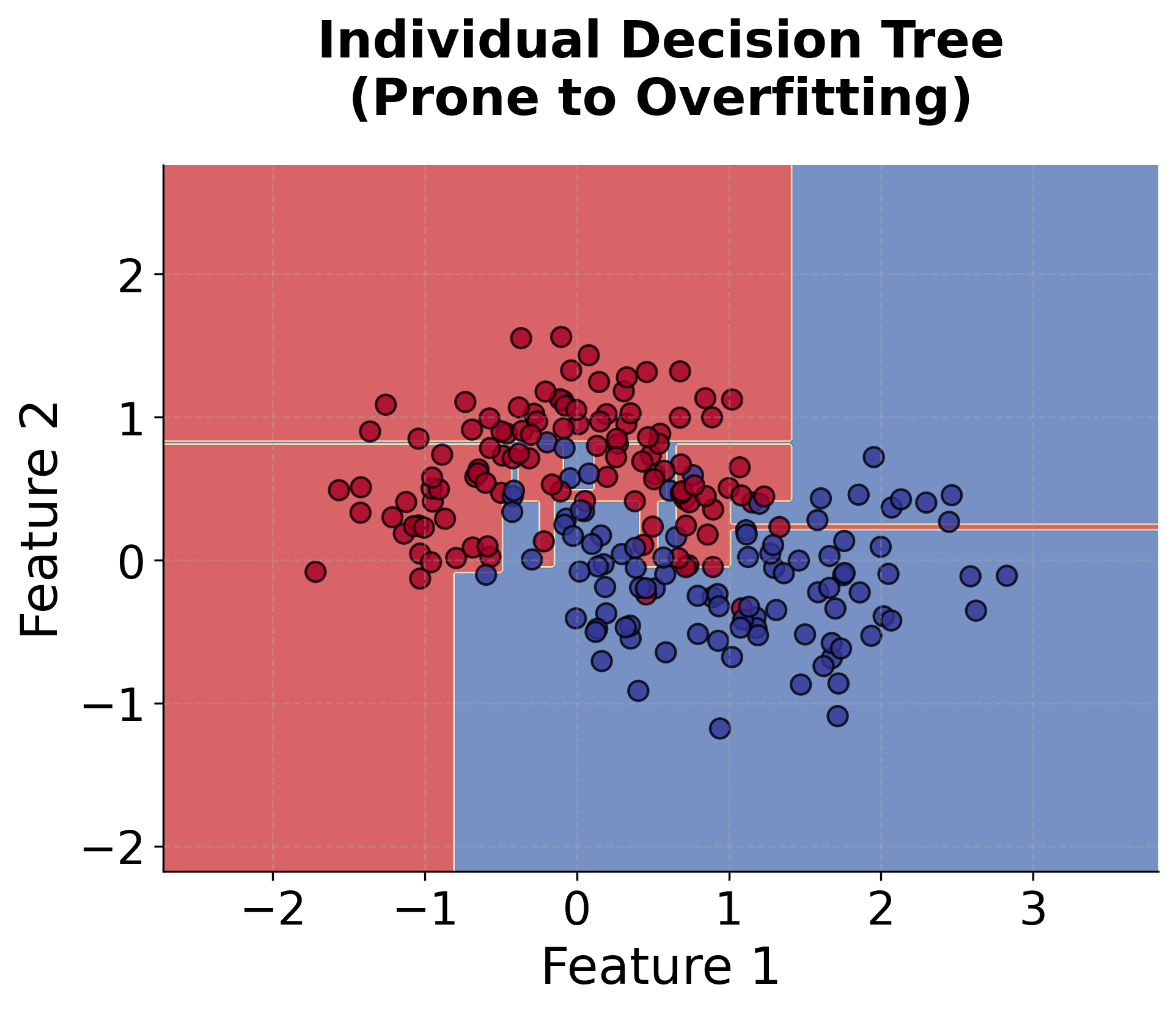
Random Forest is a powerful ensemble learning method that combines multiple decision trees to create a more robust and accurate predictive model. The core idea behind Random Forest is to build many individual decision trees, each trained on a slightly different subset of the data, and then combine their predictions through voting (for classification) or averaging (for regression). This approach addresses many of the limitations of individual decision trees, such as overfitting and high variance, by leveraging the wisdom of crowds principle.

The "random" in Random Forest comes from two key sources of randomness: bootstrap sampling (where each tree is trained on a random subset of the original data) and random feature selection (where each tree only considers a random subset of features when making splits). This randomness ensures that each tree in the forest learns different patterns from the data, making the ensemble more diverse and robust than any single tree.

In simple terms, Random Forest is like asking a group of experts to make predictions, where each expert has seen slightly different information and focuses on different aspects of the problem. Instead of relying on one expert's opinion, we combine all their predictions to get a more reliable and accurate result. This approach typically produces models that are more accurate, more stable, and less prone to overfitting than individual decision trees.

Advantages

Random Forest offers several compelling advantages that make it one of the most popular machine learning algorithms. First, it provides excellent predictive performance across a wide variety of problems without requiring extensive hyperparameter tuning. The algorithm is robust to overfitting due to the ensemble effect and the randomness introduced through bootstrap sampling and feature selection. This makes Random Forest particularly valuable when you have limited time for model tuning or when working with complex datasets where other algorithms might struggle.

Additionally, Random Forest handles both classification and regression problems seamlessly, and it can work with mixed data types (numerical and categorical features) without requiring extensive preprocessing. The algorithm is relatively insensitive to outliers and missing values, making it robust for real-world datasets that often contain imperfect data. Random Forest also provides built-in feature importance measures, allowing you to understand which features are most influential in making predictions, which is valuable for both model interpretation and feature selection.

Another significant advantage is that Random Forest can handle high-dimensional data effectively and doesn't require feature scaling, unlike many other algorithms. The algorithm is also computationally efficient and can be easily parallelized, making it suitable for large datasets. Finally, Random Forest provides uncertainty estimates through the variance of predictions across trees, which can be valuable for understanding prediction confidence.

Disadvantages

Despite its many strengths, Random Forest has some limitations that are important to consider. One of the main drawbacks is that Random Forest models can be quite large and memory-intensive, especially when using many trees or when dealing with high-dimensional data. This can make the models slow to deploy in production environments or when memory is constrained.

Another limitation is that while Random Forest provides feature importance measures, the individual trees in the forest are not easily interpretable, making it difficult to understand the exact decision-making process. The ensemble nature of the algorithm means that you can't easily trace how a specific prediction was made, which can be problematic in applications where interpretability is crucial.

Random Forest can also struggle with very sparse data or when there are strong linear relationships in the data, where simpler linear models might perform better. The algorithm tends to overfit when dealing with very noisy datasets, and it may not perform well when the signal-to-noise ratio is very low. Additionally, Random Forest can be biased towards features with many categories or high cardinality, potentially giving them more importance than they deserve.

Finally, while Random Forest is generally robust, it can still be sensitive to the quality of the input data. If the training data contains systematic biases or errors, these biases will be reflected in the ensemble's predictions. The algorithm also requires careful tuning of hyperparameters like the number of trees, maximum depth, and minimum samples per leaf to achieve optimal performance.

Formula

The mathematical foundation of Random Forest involves understanding how individual decision trees are combined to form the ensemble. Let's break this down step by step, starting with the basic structure and progressing to the complete ensemble formulation.

Individual Decision Tree

Each tree in the Random Forest is a decision tree that makes predictions by recursively partitioning the feature space. We denote the $b$-th tree in the ensemble as $T_b$, where the capital $T$ represents the tree as a function or mapping from input features to a prediction. For a given input $\mathbf{x}$, this tree produces a prediction $\hat{y}_b = T_b(\mathbf{x})$. Here, $T_b(\mathbf{x})$ means we apply the $b$-th decision tree to the input $\mathbf{x}$ to obtain its predicted value.

The prediction from a single tree can be written as:

$\hat{y}_b = \sum_{i=1}^{n} w_i(\mathbf{x}) \cdot y_i$

where:

• $\hat{y}_b$: Prediction from the $b$-th tree in the ensemble
• $n$: Total number of training observations in the dataset
• $w_i(\mathbf{x})$: Weight assigned to training observation $i$ when making a prediction for input $\mathbf{x}$
• $y_i$: Target value (actual outcome) of training observation $i$
• $\mathbf{x}$: Input feature vector for which we are making a prediction

The weights $w_i(\mathbf{x})$ are determined by which leaf node the input $\mathbf{x}$ falls into. If $\mathbf{x}$ falls into the same leaf as training observation $i$, then $w_i(\mathbf{x}) = \frac{1}{n_{\text{leaf}}}$ where $n_{\text{leaf}}$ is the number of training observations in that leaf. Otherwise, $w_i(\mathbf{x}) = 0$. The weights always sum to 1: $\sum_{i=1}^{n} w_i(\mathbf{x}) = 1$.

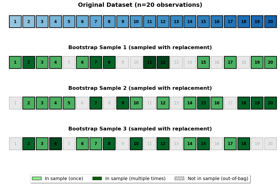
Bootstrap Sampling

Each tree is trained on a bootstrap sample of the original training data. A bootstrap sample is created by randomly sampling $n$ observations with replacement from the original $n$ observations. This means some observations may appear multiple times in a bootstrap sample, while others may not appear at all.

Mathematically, for tree $b$, we create a bootstrap sample $\mathcal{D}_b$ by sampling with replacement from the original dataset $\mathcal{D} = \{(\mathbf{x}_1, y_1), (\mathbf{x}_2, y_2), \ldots, (\mathbf{x}_n, y_n)\}$.

The probability that a specific observation is included in a bootstrap sample is:

$P(\text{observation } i \text{ in bootstrap sample}) = 1 - \left(1 - \frac{1}{n}\right)^n$

where:

• $n$: Total number of observations in the original dataset
• $P(\text{observation } i \text{ in bootstrap sample})$: Probability that observation $i$ appears at least once in a bootstrap sample of size $n$

As $n$ becomes large, this probability approaches $1 - e^{-1} \approx 0.632$, meaning approximately 63.2% of the original observations appear in each bootstrap sample.

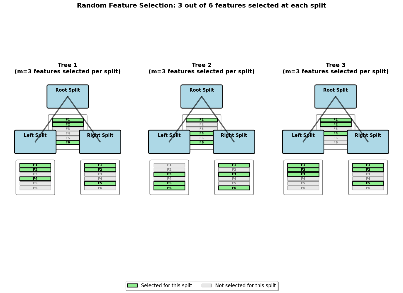
Random Feature Selection

At each split in each tree, only a random subset of features is considered for the split. If the original dataset has $p$ features, then at each split, we randomly select $m$ features where typically $m = \sqrt{p}$ for classification or $m = p/3$ for regression.

This random feature selection introduces additional diversity among the trees and helps prevent overfitting to specific features.

Ensemble Prediction

The final Random Forest prediction combines the predictions from all $B$ trees in the ensemble. For regression problems, the prediction is the average of all tree predictions:

$\hat{y} = \frac{1}{B} \sum_{b=1}^{B} \hat{y}_b = \frac{1}{B} \sum_{b=1}^{B} T_b(\mathbf{x})$

where:

• $\hat{y}$: Final ensemble prediction for input $\mathbf{x}$
• $B$: Total number of trees in the Random Forest
• $\hat{y}_b$: Prediction from the $b$-th tree
• $T_b(\mathbf{x})$: Function representing the $b$-th tree applied to input $\mathbf{x}$

For classification problems, the prediction is made by taking a majority vote among all the trees in the forest. This means that each tree "votes" for a class label, and the class that receives the most votes is chosen as the final prediction.

In mathematical terms, this is called taking the "mode" of the predicted class labels, where the mode is simply the value that appears most frequently in a set. If there is a tie, some implementations may break the tie randomly or by another rule.

$\hat{y} = \text{mode}\{T_1(\mathbf{x}), T_2(\mathbf{x}), \ldots, T_B(\mathbf{x})\}$

Or, if we consider the probability of each class:

$\hat{p}_k = \frac{1}{B} \sum_{b=1}^{B} P_b(\text{class } k | \mathbf{x})$

where:

• $\hat{p}_k$: Estimated probability that input $\mathbf{x}$ belongs to class $k$
• $P_b(\text{class } k | \mathbf{x})$: Probability that tree $b$ assigns to class $k$ for input $\mathbf{x}$

Complete Random Forest Algorithm

Putting it all together, the Random Forest algorithm can be written as:

Input: Training data $\mathcal{D} = \{(\mathbf{x}_1, y_1), (\mathbf{x}_2, y_2), \ldots, (\mathbf{x}_n, y_n)\}$, number of trees $B$, number of features to consider at each split $m$

For $b = 1$ to $B$:

1. Create bootstrap sample $\mathcal{D}_b$ by sampling $n$ observations with replacement from $\mathcal{D}$
2. Train decision tree $T_b$ on $\mathcal{D}_b$ using the following splitting rule:
   • At each split, randomly select $m$ features from the $p$ available features
   • Choose the best split among the $m$ selected features
   • Continue until stopping criteria are met (e.g., minimum samples per leaf, maximum depth)

Output: Ensemble of trees $\{T_1, T_2, \ldots, T_B\}$

Prediction: For new input $\mathbf{x}$:

• Regression: $\hat{y} = \frac{1}{B} \sum_{b=1}^{B} T_b(\mathbf{x})$
• Classification: $\hat{y} = \text{mode}\{T_1(\mathbf{x}), T_2(\mathbf{x}), \ldots, T_B(\mathbf{x})\}$

Mathematical Properties

Random Forests possess several key mathematical properties that help explain their effectiveness. One of the most important is the bias-variance decomposition. When we use a single decision tree, the model tends to have low bias but high variance, meaning it can fit the training data closely but may not generalize well to new data. By averaging the predictions of many trees, Random Forests reduce the variance component of the error while keeping the bias relatively low. The overall error of the ensemble can be expressed as:

$\text{Error} = \text{Bias}^2 + \text{Variance} + \text{Noise}$

This formula shows that the total prediction error consists of three parts: the squared bias (how far the average model prediction is from the true values), the variance (how much the predictions fluctuate for different training sets), and the irreducible noise inherent in the data. By averaging over multiple trees, Random Forests specifically target and reduce the variance term, leading to more stable and reliable predictions.

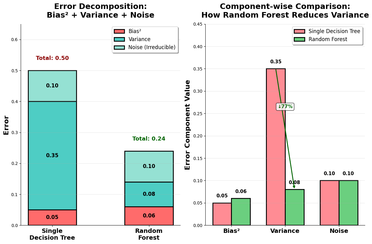
Another important property is the concept of out-of-bag (OOB) error. Because each tree in the forest is trained on a bootstrap sample, about 37% of the original data points are left out of the training set for any given tree. These unused data points, known as "out-of-bag" observations, can be used to estimate the model's generalization error without the need for a separate validation set. This built-in validation approach provides an efficient way to assess model performance.

Finally, Random Forests offer a natural way to measure feature importance. By tracking how much each feature contributes to reducing impurity—such as Gini impurity for classification tasks or mean squared error for regression—across all trees in the forest, we can identify which features are most influential in making predictions. This helps us interpret the model and understand which variables are driving its decisions.

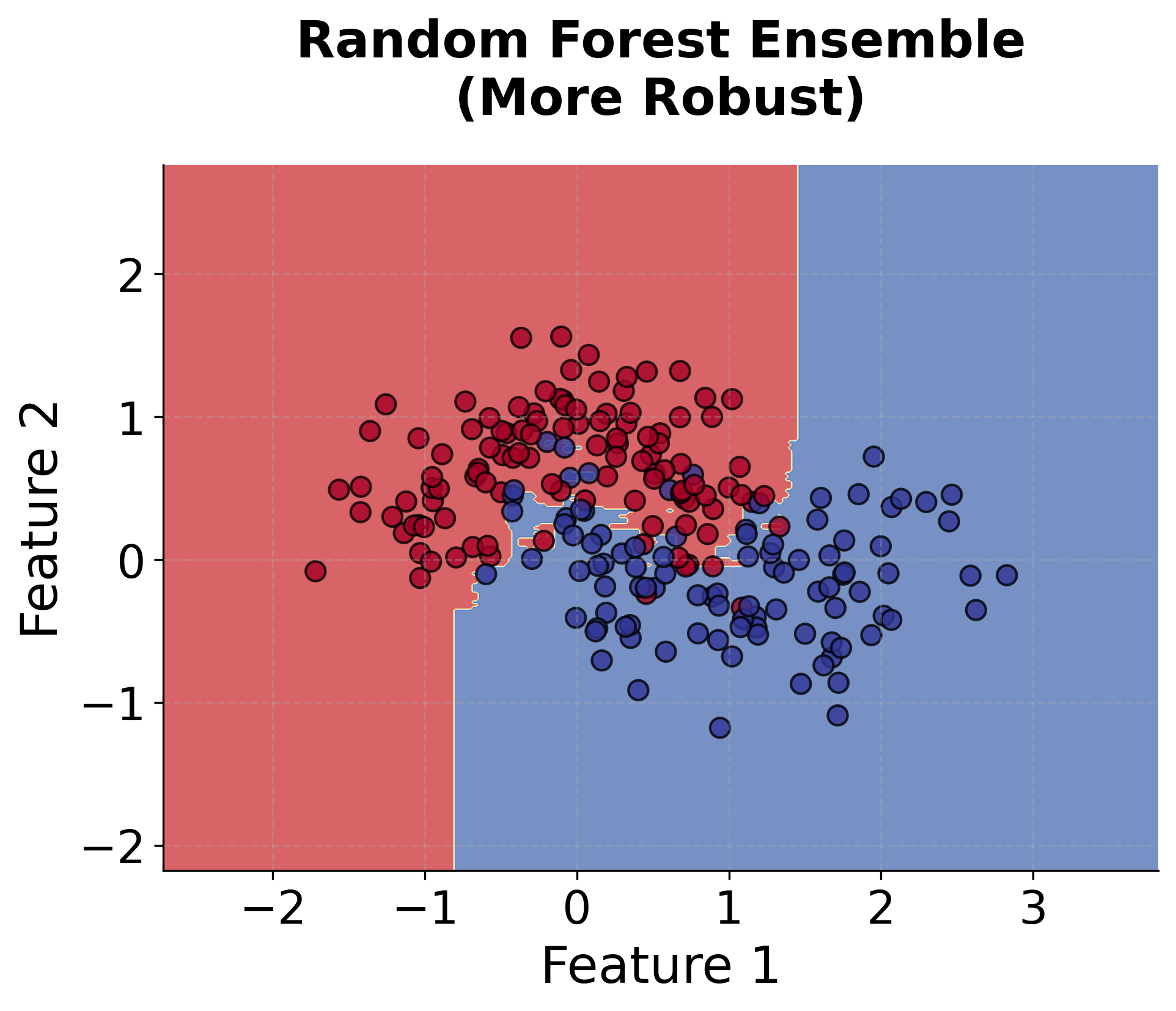
Visualizing Random Forest

Let's create visualizations that demonstrate how Random Forest works and how it differs from individual decision trees.

Now let's visualize how the number of trees affects the Random Forest performance:

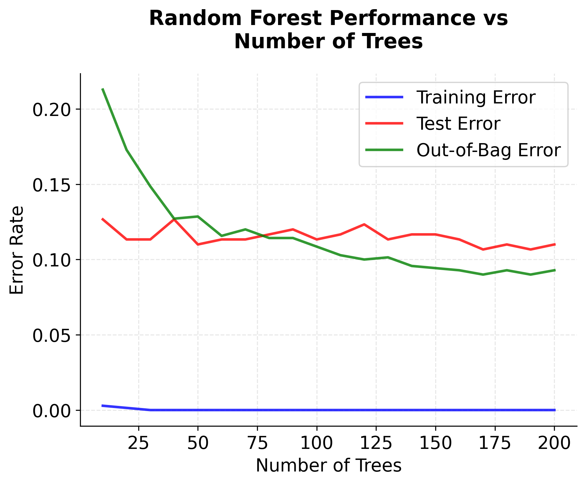
Note on Out-of-Bag (OOB) Error: The OOB error calculation requires a sufficient number of trees to provide reliable estimates. With very few trees, some observations may not be "out-of-bag" for any tree, making OOB scores unavailable. This is why we start the visualization from 10 trees rather than 1, and why scikit-learn may issue warnings about insufficient OOB samples when using very small numbers of trees. The OOB error provides a useful estimate of generalization performance without needing a separate validation set, but it becomes more reliable as the number of trees increases.

Example - Classification

Let's work through a detailed step-by-step example of Random Forest using a simple dataset. Suppose we want to predict whether a customer will purchase a product based on their age, income, and years of experience.

Given Data:

• Age: [25, 30, 35, 40, 45, 50, 55, 60]
• Income (thousands): [40, 50, 60, 70, 80, 90, 100, 110]
• Years of Experience: [2, 5, 8, 12, 15, 18, 20, 22]
• Purchase (1) or No Purchase (0): [0, 0, 1, 1, 1, 1, 1, 1]

Step 1: Create Bootstrap Samples

Random Forest creates multiple bootstrap samples from the original data. Let's create 3 bootstrap samples for illustration:

Bootstrap Sample 1: [1, 2, 3, 4, 5, 6, 7, 8] → [1, 1, 2, 3, 4, 5, 6, 7]

Bootstrap Sample 2: [1, 2, 3, 4, 5, 6, 7, 8] → [2, 3, 4, 4, 5, 6, 7, 8]

Bootstrap Sample 3: [1, 2, 3, 4, 5, 6, 7, 8] → [1, 2, 3, 5, 6, 7, 8, 8]

Note: In practice, bootstrap samples are created by sampling with replacement, so some observations may appear multiple times while others may not appear at all.

Step 2: Train Individual Trees

Each tree is trained on its bootstrap sample using random feature selection. At each split, only a random subset of features is considered.

Tree 1 (trained on Bootstrap Sample 1):

• Root split: Age ≤ 35 (using Age and Income features)
• Left child: Age ≤ 35 → No Purchase (0)
• Right child: Age > 35 → Purchase (1)

Tree 2 (trained on Bootstrap Sample 2):

• Root split: Income ≤ 75 (using Income and Experience features)
• Left child: Income ≤ 75 → No Purchase (0)
• Right child: Income > 75 → Purchase (1)

Tree 3 (trained on Bootstrap Sample 3):

• Root split: Experience ≤ 10 (using Age and Experience features)
• Left child: Experience ≤ 10 → No Purchase (0)
• Right child: Experience > 10 → Purchase (1)

Step 3: Make Predictions

For a new customer with Age=42, Income=85, Experience=14:

Tree 1 Prediction: Age=42 > 35 → Right child → Purchase (1)

Tree 2 Prediction: Income=85 > 75 → Right child → Purchase (1)

Tree 3 Prediction: Experience=14 > 10 → Right child → Purchase (1)

Step 4: Combine Predictions

Random Forest combines the predictions from all trees:

• Tree 1: Purchase (1)
• Tree 2: Purchase (1)
• Tree 3: Purchase (1)

Final Prediction: Majority vote = Purchase (1)

Step 5: Calculate Probabilities

The probability of purchase is the proportion of trees that predicted purchase: $P(\text{Purchase}) = \frac{3}{3} = 1.0$

Step 6: Feature Importance

Random Forest calculates feature importance based on how much each feature contributes to reducing impurity across all trees:

• Age: Used in Tree 1 and Tree 3, contributes to 2/3 of the splits
• Income: Used in Tree 2, contributes to 1/3 of the splits
• Experience: Used in Tree 3, contributes to 1/3 of the splits

Normalized Feature Importance:

• Age: 2/3 ≈ 0.67
• Income: 1/3 ≈ 0.33
• Experience: 1/3 ≈ 0.33

This example demonstrates how Random Forest combines multiple decision trees to make more robust predictions. Each tree learns different patterns from the data, and the ensemble approach reduces the risk of overfitting while maintaining good predictive performance.

Example - Regression

Now let's work through a regression example where we want to predict house prices based on house size, number of bedrooms, and number of bathrooms.

Given Data:

• House Size (sq ft): [1200, 1500, 1800, 2000, 2200, 2500, 2800, 3000]
• Bedrooms: [2, 3, 3, 4, 4, 4, 5, 5]
• Bathrooms: [1, 2, 2, 2, 3, 3, 3, 4]
• House Price (thousands): [180, 220, 260, 300, 340, 380, 420, 460]

Step 1: Create Bootstrap Samples

For regression, we create bootstrap samples just like in classification:

Bootstrap Sample 1: [1, 2, 3, 4, 5, 6, 7, 8] → [1, 1, 2, 3, 4, 5, 6, 7]

Bootstrap Sample 2: [1, 2, 3, 4, 5, 6, 7, 8] → [2, 3, 4, 4, 5, 6, 7, 8]

Bootstrap Sample 3: [1, 2, 3, 4, 5, 6, 7, 8] → [1, 2, 3, 5, 6, 7, 8, 8]

Step 2: Train Individual Trees

Each tree is trained on its bootstrap sample using random feature selection and regression splitting criteria (typically mean squared error).

Tree 1 (trained on Bootstrap Sample 1):

• Root split: House Size ≤ 2000 (using House Size and Bedrooms features)
• Left child: House Size ≤ 2000 → Average Price = 240
• Right child: House Size > 2000 → Average Price = 400

Tree 2 (trained on Bootstrap Sample 2):

• Root split: Bedrooms ≤ 3 (using Bedrooms and Bathrooms features)
• Left child: Bedrooms ≤ 3 → Average Price = 220
• Right child: Bedrooms > 3 → Average Price = 380

Tree 3 (trained on Bootstrap Sample 3):

• Root split: Bathrooms ≤ 2 (using House Size and Bathrooms features)
• Left child: Bathrooms ≤ 2 → Average Price = 250
• Right child: Bathrooms > 2 → Average Price = 380

Step 3: Make Predictions

For a new house with Size=2100, Bedrooms=4, Bathrooms=3:

Tree 1 Prediction: Size=2100 > 2000 → Right child → Price = 400

Tree 2 Prediction: Bedrooms=4 > 3 → Right child → Price = 380

Tree 3 Prediction: Bathrooms=3 > 2 → Right child → Price = 380

Step 4: Combine Predictions

Random Forest combines the predictions from all trees by averaging:

• Tree 1: 400
• Tree 2: 380
• Tree 3: 380

Final Prediction: Average = (400 + 380 + 380) / 3 = 386.67

Step 5: Calculate Prediction Variance

The variance of predictions across trees provides an estimate of prediction uncertainty:

$\text{Variance} = \frac{1}{B-1} \sum_{b=1}^{B} (\hat{y}_b - \bar{\hat{y}})^2$

where:

• $\text{Variance}$: Sample variance of predictions across all trees
• $B$: Total number of trees in the Random Forest (3 in this example)
• $\hat{y}_b$: Prediction from the $b$-th tree
• $\bar{\hat{y}}$: Mean prediction across all trees, calculated as $\bar{\hat{y}} = \frac{1}{B} \sum_{b=1}^{B} \hat{y}_b$

For our example: $\text{Variance} = \frac{1}{2} [(400-386.67)^2 + (380-386.67)^2 + (380-386.67)^2]$
$= \frac{1}{2} [177.78 + 44.44 + 44.44] = 133.33$

Step 6: Feature Importance

Random Forest calculates feature importance based on how much each feature contributes to reducing mean squared error across all trees:

• House Size: Used in Tree 1 and Tree 3, contributes to 2/3 of the splits
• Bedrooms: Used in Tree 2, contributes to 1/3 of the splits
• Bathrooms: Used in Tree 2 and Tree 3, contributes to 2/3 of the splits

Normalized Feature Importance:

• House Size: 2/3 ≈ 0.67
• Bedrooms: 1/3 ≈ 0.33
• Bathrooms: 2/3 ≈ 0.67

This regression example demonstrates how Random Forest provides both point predictions and uncertainty estimates through the variance of individual tree predictions. The ensemble approach helps create more stable and reliable predictions compared to individual decision trees.

Implementation in Scikit-learn

Random Forest is implemented in scikit-learn through the RandomForestClassifier and RandomForestRegressor classes. Let's implement a complete example with proper preprocessing and evaluation:

Now let's implement a regression example:

Hyperparameter Tuning

Random Forest has several important hyperparameters that can significantly affect performance:

Key Parameters

Below are some of the main parameters that affect how Random Forest works and performs.

• n_estimators: Number of trees in the forest (default: 100). More trees generally improve performance but increase computation time. Start with 100 and increase if cross-validation shows improvement. Values between 100-500 work well for most datasets.
• max_depth: Maximum depth of each tree (default: None, meaning nodes expand until all leaves are pure or contain fewer than min_samples_split samples). Limiting depth helps prevent overfitting. Try values like 10, 15, or 20 for complex datasets.
• min_samples_split: Minimum number of samples required to split an internal node (default: 2). Higher values prevent overfitting by requiring more data for splits. Values of 5-10 work well for most datasets.
• min_samples_leaf: Minimum number of samples required in a leaf node (default: 1). Higher values smooth the model and prevent overfitting. Values of 2-4 are commonly used.
• max_features: Number of features to consider when looking for the best split (default: 'sqrt' for classification, 1.0 for regression). Controls the diversity of trees in the forest. Use 'sqrt' for classification and 'log2' or p/3 for regression.
• bootstrap: Whether to use bootstrap samples when building trees (default: True). Setting to False uses the entire dataset for each tree, which reduces diversity but may be useful in some cases.
• oob_score: Whether to use out-of-bag samples to estimate generalization performance (default: False). Set to True to get an unbiased estimate without needing a separate validation set.
• random_state: Seed for reproducibility (default: None). Set to an integer to ensure consistent results across runs.
• n_jobs: Number of CPU cores to use for parallel training (default: None, meaning 1 core). Set to -1 to use all available cores for faster training.

Key Methods

The following are the most commonly used methods for interacting with Random Forest models.

• fit(X, y): Trains the Random Forest on the training data X and target values y. Each tree is trained on a bootstrap sample of the data.
• predict(X): Returns predicted class labels (classification) or values (regression) for input data X by aggregating predictions from all trees.
• predict_proba(X): Returns probability estimates for each class (classification only). Useful for setting custom decision thresholds or understanding prediction confidence.
• score(X, y): Returns the mean accuracy (classification) or R² score (regression) on the given test data and labels.
• feature_importances_: Attribute (not a method) that provides the importance of each feature, calculated as the mean decrease in impurity across all trees.

Practical Implications

Random Forest is particularly effective in scenarios where predictive accuracy is prioritized over model interpretability. In customer churn prediction, for example, Random Forest excels at identifying complex patterns in customer behavior data that might involve non-linear relationships and interactions between features. The algorithm's ability to handle mixed data types makes it well-suited for business applications where datasets often contain both numerical metrics and categorical attributes.

The algorithm is also valuable in medical diagnosis applications, where it can process diverse patient data including lab results, demographic information, and medical history to make predictions. Random Forest's robustness to noisy data and outliers is particularly beneficial in healthcare settings where measurement errors and data quality issues are common. The built-in feature importance measures help medical professionals understand which factors contribute most to diagnoses, supporting clinical decision-making.

In financial risk assessment and fraud detection, Random Forest's ensemble approach provides stable predictions even when dealing with imbalanced datasets and evolving patterns. The algorithm can effectively identify fraudulent transactions by learning from historical patterns while remaining robust to the high false positive rates that plague simpler models. Its ability to provide probability estimates through predict_proba allows organizations to set custom decision thresholds based on their risk tolerance.

Best Practices

To achieve optimal results with Random Forest, start with default parameters and use them as a baseline before tuning. Begin with 100 trees (n_estimators=100) and increase if cross-validation scores show improvement, though values beyond 500 trees rarely provide significant gains. For the number of features to consider at each split, use the square root of total features for classification problems and one-third of total features for regression problems, as these defaults typically work well across diverse datasets.

When tuning hyperparameters, focus on max_depth, min_samples_split, and min_samples_leaf to control model complexity. Limiting tree depth to values between 10 and 20 often prevents overfitting while maintaining predictive power. Setting min_samples_leaf to 2-4 creates smoother decision boundaries and improves generalization. Use out-of-bag scoring (oob_score=True) to estimate model performance without requiring a separate validation set, which is particularly useful when data is limited.

For evaluation, combine multiple metrics rather than relying on a single measure. For classification, examine both accuracy and ROC AUC to understand overall performance and class separation. For regression, compare R² scores with RMSE to assess both explained variance and prediction error magnitude. Use cross-validation with at least 5 folds to obtain robust performance estimates. Analyze feature importance scores to identify the most influential predictors, but be cautious when features are highly correlated, as importance may be distributed among correlated features rather than concentrated in the most relevant ones.

Data Requirements and Preprocessing

Random Forest works directly with numerical features without requiring standardization or normalization, since decision trees make splits based on feature values rather than distances. This makes the algorithm easier to apply compared to distance-based methods like k-nearest neighbors or support vector machines. However, the algorithm does require sufficient training data to build robust trees. As a general guideline, datasets with at least several hundred observations tend to produce more reliable models, though Random Forest can work with smaller datasets when tree depth is appropriately constrained.

Missing values require attention despite Random Forest's theoretical ability to handle them through surrogate splits. In practice, scikit-learn's implementation does not support missing values directly, so imputation is necessary. Simple strategies like mean or median imputation work well for numerical features, while mode imputation or creating a separate "missing" category can be effective for categorical variables. For datasets with substantial missing data, consider using more sophisticated imputation methods like K-nearest neighbors imputation or iterative imputation.

Categorical variables need encoding before use with scikit-learn's Random Forest implementation. One-hot encoding works well for low-cardinality categorical features (those with fewer than 10-15 unique values), creating binary indicator variables for each category. For high-cardinality features, consider target encoding or frequency encoding to avoid creating too many sparse features. Be cautious with high-cardinality categorical variables, as they can receive artificially inflated importance scores due to the increased number of potential split points they provide.

Common Pitfalls

One frequent mistake is using default settings without considering the specific characteristics of your dataset. While Random Forest's defaults work reasonably well in many cases, they may not be optimal for your particular problem. For small datasets (fewer than 1,000 observations), the default tree depth may lead to overfitting. In such cases, explicitly setting max_depth to values between 5 and 10 and increasing min_samples_leaf to 5 or more can improve generalization. Conversely, for very large datasets, the default settings may underfit, requiring deeper trees or more features per split.

Another common issue involves misinterpreting feature importance scores, particularly when features are highly correlated. When two features contain similar information, Random Forest may arbitrarily assign importance to one over the other, or split the importance between them. This can lead to incorrect conclusions about which features are truly driving predictions. To address this, examine correlation matrices before training and consider removing highly correlated features (correlation > 0.9) or using permutation importance, which tends to be more stable in the presence of correlated features.

Class imbalance in classification problems can significantly impact Random Forest performance, as the algorithm tends to favor the majority class. When one class represents less than 10-20% of the data, the model may achieve high overall accuracy while performing poorly on the minority class. Address this by using the class_weight='balanced' parameter, which automatically adjusts weights inversely proportional to class frequencies, or by using stratified sampling techniques to ensure balanced representation in bootstrap samples. Additionally, evaluate performance using metrics appropriate for imbalanced data, such as F1-score, precision-recall curves, or ROC AUC, rather than relying solely on accuracy.

Computational Considerations

Random Forest's training time scales linearly with the number of trees and roughly linearly with the number of training samples, making it computationally intensive for large datasets. For datasets with more than 100,000 observations, training time can become substantial even with parallelization. The algorithm's time complexity is approximately O(B × n × log(n) × m), where B is the number of trees, n is the number of samples, and m is the number of features considered at each split. This means that doubling the dataset size roughly doubles training time, while doubling the number of trees exactly doubles training time.

Memory requirements can be significant, particularly for models with many deep trees or high-dimensional feature spaces. Each tree stores split information for every internal node, and the total model size grows with both the number of trees and their depth. For datasets with more than 1,000 features or when using more than 500 trees, model sizes can exceed several hundred megabytes. To manage memory usage, consider limiting tree depth, reducing the number of trees, or using feature selection to decrease dimensionality before training.

Parallelization provides substantial speedups for both training and prediction when multiple CPU cores are available. Setting n_jobs=-1 distributes tree training across all available cores, often reducing training time by a factor close to the number of cores. However, prediction time scales linearly with the number of trees regardless of parallelization in scikit-learn's implementation, as each tree is evaluated sequentially for a given input. For real-time applications requiring predictions in milliseconds, consider using fewer trees (50-100) or exploring alternative implementations that support parallel prediction.

Performance and Deployment Considerations

Model evaluation should focus on metrics appropriate for your specific problem and business context. For classification tasks, use ROC AUC when class probabilities matter and you need to evaluate performance across different decision thresholds. F1-score is more appropriate when you need to balance precision and recall, particularly in imbalanced datasets. For regression tasks, R² provides an interpretable measure of explained variance, while RMSE gives prediction error in the original units of the target variable, making it easier to assess practical significance.

Cross-validation provides more reliable performance estimates than a single train-test split, particularly for smaller datasets. Use stratified k-fold cross-validation for classification to ensure each fold maintains the original class distribution. For time series data, use time-based splitting where training data precedes test data to avoid lookahead bias. When computational resources are limited, 5-fold cross-validation typically provides a good balance between reliability and computational cost.

Deploying Random Forest models in production requires consideration of both model size and inference latency. Serialized models can range from a few megabytes to several gigabytes depending on the number and depth of trees. For deployment in resource-constrained environments, use model compression techniques such as reducing the number of trees while monitoring performance degradation, or consider exporting the model to more efficient formats. Monitor prediction latency in production, as inference time increases linearly with the number of trees and can become problematic for high-throughput applications requiring sub-millisecond predictions.

Summary

Random Forest is a powerful and versatile ensemble learning algorithm that combines multiple decision trees to create robust and accurate predictive models. By leveraging bootstrap sampling and random feature selection, Random Forest addresses many of the limitations of individual decision trees while maintaining good predictive performance across a wide variety of problems.

The key strength of Random Forest lies in its ability to reduce overfitting through the ensemble effect while maintaining low bias. The algorithm is robust to outliers, missing values, and noisy data, making it suitable for real-world datasets that often contain imperfect information. Additionally, Random Forest provides built-in feature importance measures that offer valuable insights into which features are most influential in making predictions.

However, Random Forest models can be large and memory-intensive, especially when using many trees or dealing with high-dimensional data. The ensemble nature of the algorithm also makes it less interpretable than individual decision trees or linear models, which can be problematic in applications where interpretability is crucial.

Despite these limitations, Random Forest remains one of the most popular and effective machine learning algorithms, serving as an excellent baseline model and often providing surprisingly good results with minimal hyperparameter tuning. Its combination of robustness, versatility, and performance makes it particularly valuable in applications where you need reliable predictions without extensive model development time, such as in exploratory data analysis, feature selection, and as a benchmark for comparing other algorithms.