InteractiveQuadratic Programming for Portfolio Optimization: Complete Guide with Python Implementation

Quadratic Programming for Portfolio OptimizationLink Copied

Portfolio optimization is one of the most fundamental problems in quantitative finance, where we seek to find the optimal allocation of assets that maximizes expected return while minimizing risk. This problem naturally lends itself to quadratic programming (QP), a mathematical optimization technique that deals with quadratic objective functions subject to linear constraints. QP balances the trade-off between risk and return through a single mathematical framework.

The modern portfolio theory, pioneered by Harry Markowitz in 1952, provides the theoretical foundation for this approach. Markowitz showed that investors can achieve better risk-adjusted returns by diversifying their portfolios rather than simply choosing the highest-returning individual assets. This diversification benefit is mathematically captured through the covariance structure of asset returns, which forms the core of the quadratic programming formulation.

Unlike linear programming, which deals with linear objective functions, quadratic programming allows us to model the non-linear relationship between portfolio risk and asset weights. This is crucial because portfolio risk (variance) grows quadratically with asset weights, making QP the natural choice for portfolio optimization problems. The quadratic nature of the risk function captures the reality that combining assets with different risk profiles creates complex interactions that linear models cannot adequately represent.

AdvantagesLink Copied

Quadratic programming for portfolio optimization offers several advantages. First, it provides a mathematically rigorous framework for balancing risk and return, allowing investors to explicitly quantify the trade-offs between these competing objectives. The quadratic objective function penalizes variance (risk) quadratically while treating returns linearly, which aligns with the mean-variance framework developed by Markowitz.

Second, QP formulations are computationally efficient and can handle large-scale problems with hundreds or even thousands of assets. Modern optimization solvers, particularly those based on interior-point methods, can solve portfolio optimization problems in milliseconds, making them suitable for real-time trading applications. This computational efficiency is important in high-frequency trading environments where portfolio rebalancing decisions need to be made rapidly.

Third, the framework is highly flexible and can accommodate various constraints that reflect real-world investment constraints. These include budget constraints (total investment must equal available capital), sector limits (maximum allocation to specific industries), liquidity constraints (minimum holdings in liquid assets), and regulatory requirements (maximum concentration in individual assets). The linear constraint structure of QP makes it straightforward to incorporate these practical considerations.

DisadvantagesLink Copied

Quadratic programming for portfolio optimization has several limitations that practitioners should be aware of. The most significant disadvantage is its sensitivity to input parameters, particularly the expected returns and covariance matrix. Small errors in these estimates can lead to significantly different optimal portfolios, a phenomenon known as the "error maximization" problem. This sensitivity makes the approach particularly challenging when dealing with noisy or limited historical data.

Another major limitation is the assumption that returns follow a normal distribution, which is often violated in real financial markets. Financial returns frequently exhibit fat tails, skewness, and time-varying volatility, making the mean-variance framework potentially misleading. During market stress periods, correlations between assets tend to increase substantially, leading to portfolio risk estimates that significantly underestimate actual risk.

The quadratic programming approach also assumes that investors have quadratic utility functions, which may not accurately represent real investor preferences. Many investors exhibit loss aversion, where the pain of losses exceeds the pleasure of equivalent gains, and this asymmetry is not captured by the symmetric quadratic utility function. Additionally, the framework assumes that all investors have the same information and expectations, which is rarely true in practice.

FormulaLink Copied

Building Intuition: Why Portfolio Risk is More Than the Sum of Its PartsLink Copied

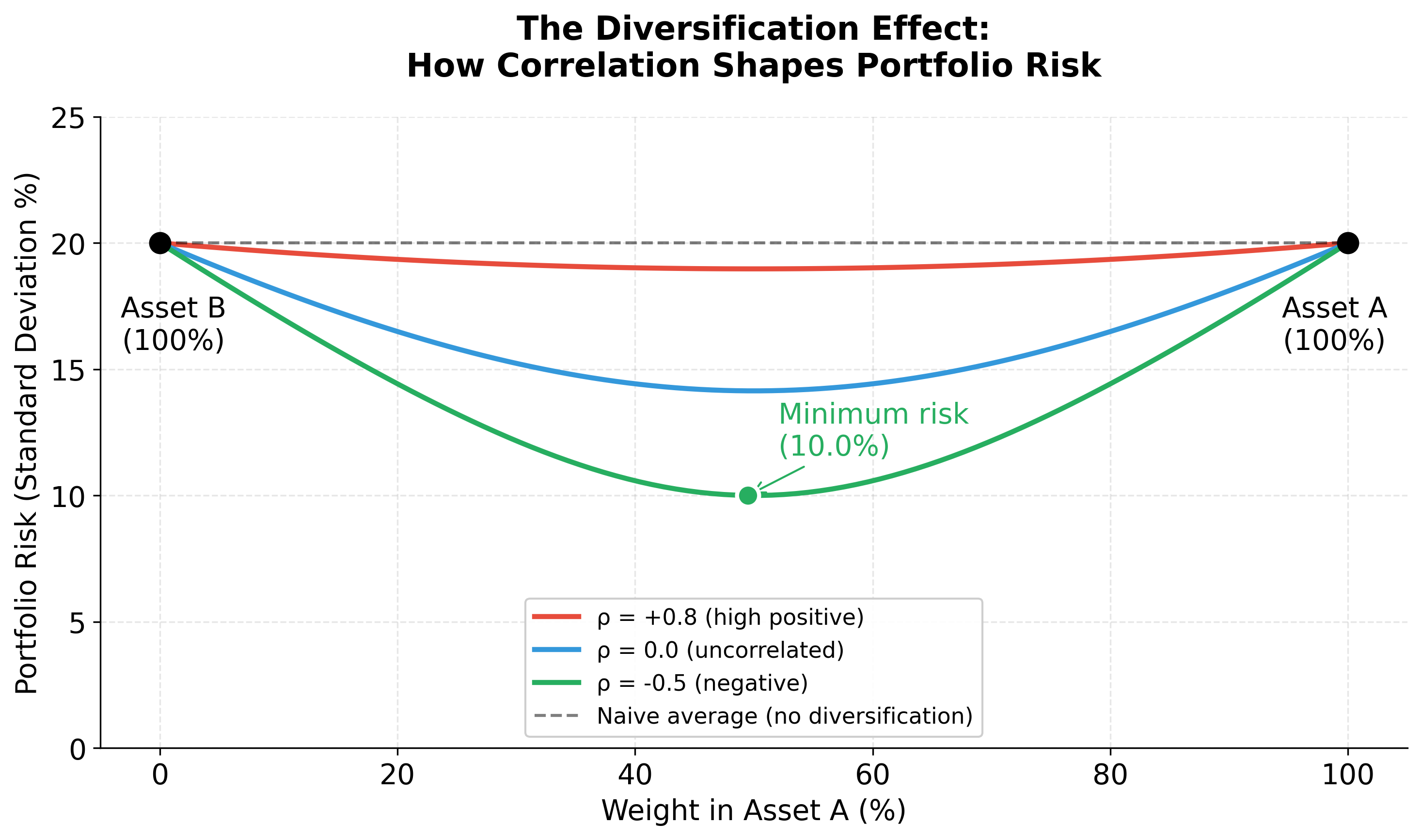
Imagine you're investing in two assets: a technology stock and a utility stock. If you put 50% of your money in each, you might naively think your portfolio risk is simply the average of their individual risks. But this intuition misses something important: how these assets move together matters just as much as how risky each one is individually.

When technology stocks crash, utility stocks often remain stable (or even rise slightly) because they represent different economic sectors. This negative correlation means your portfolio is less risky than the simple average would suggest, as the losses in one asset are partially offset by stability in the other. Conversely, if both assets tend to move together (positive correlation), your portfolio risk is amplified beyond the simple average.

This fundamental insight, that portfolio risk depends on both individual asset risks and their relationships, is why we need a mathematical framework that captures these interactions. Linear models simply cannot represent this reality, which is why portfolio optimization requires quadratic programming.

From Intuition to Mathematics: The Portfolio Variance FormulaLink Copied

Now that we've seen how correlation shapes portfolio risk, let's build the mathematical framework that captures this insight. We'll proceed step by step, starting with the most intuitive representation and gradually moving toward the matrix formulation that powers modern optimization algorithms.

Step 1: Understanding What We're Measuring

Portfolio variance measures how much the portfolio's return fluctuates over time. A high variance means the portfolio value experiences large swings, while low variance indicates more stable returns. Our goal is to construct a portfolio that achieves our desired return while minimizing this variance.

Step 2: The Building Blocks

Before we can express portfolio variance mathematically, we need to define our components:

• $w_i$: The weight (proportion) of asset $i$ in the portfolio, where $i \in \{1, 2, \ldots, n\}$. If $w_i = 0.3$, then 30% of our capital is invested in asset $i$. These weights must satisfy $\sum_{i=1}^{n} w_i = 1$ (100% of capital allocated).
• $\sigma_{ij}$: The covariance between assets $i$ and $j$, where $i, j \in \{1, 2, \ldots, n\}$. This measures how the returns of these two assets move together. When $i = j$, we have $\sigma_{ii} = \sigma_i^2$, which is the variance of asset $i$ (how much asset $i$'s return fluctuates on its own). Note that $\sigma_{ij} = \sigma_{ji}$ (covariance is symmetric).
• $\mu_i$: The expected return of asset $i$ (the average return we anticipate), where $i \in \{1, 2, \ldots, n\}$.
• $n$: The total number of assets in the portfolio.

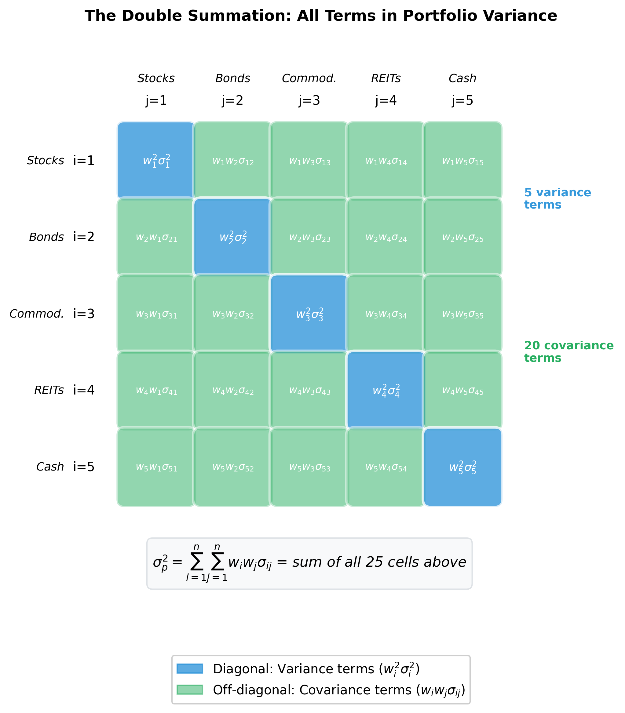
Step 3: Why a Double Summation?

The portfolio variance formula uses a double summation to capture every possible interaction between assets:

Let's break this down to understand why both summations are necessary:

1. When $i = j$: We're looking at terms like $w_i w_i \sigma_{ii} = w_i^2 \sigma_i^2$, where $\sigma_{ii} = \sigma_i^2$ is the variance of asset $i$. This captures how each asset's own variance contributes to portfolio risk, weighted by the square of its portfolio weight. Notice the squared weight. This is important because doubling your position in an asset quadruples its contribution to portfolio variance (risk grows quadratically with position size).

2. When $i \neq j$: We're looking at terms like $w_i w_j \sigma_{ij}$ where $i \neq j$. These cross-terms capture the diversification effects. If $\sigma_{ij} < 0$ (negative correlation), this term reduces portfolio variance. If $\sigma_{ij} > 0$ (positive correlation), it increases variance. If $\sigma_{ij} = 0$ (uncorrelated assets), the term contributes zero to portfolio variance.

The double summation ensures we consider all $n^2$ possible pairs of assets, not just the $n$ individual assets. This comprehensive accounting is what makes the formula mathematically complete and practically powerful.

Step 4: The Expected Return Formula

While portfolio variance requires the complexity of a double summation, expected portfolio return is simple. It's just the weighted average:

where:

• $\mu_p$: The expected return of the portfolio (a scalar)
• $w_i$: The weight of asset $i$ in the portfolio
• $\mu_i$: The expected return of asset $i$

This linear relationship follows directly from the definition of expected value. Consider a two-asset example:

• Asset 1: weight $w_1 = 0.3$ (30%), expected return $\mu_1 = 0.10$ (10%)
• Asset 2: weight $w_2 = 0.7$ (70%), expected return $\mu_2 = 0.05$ (5%)

The portfolio's expected return is:

which equals 6.5%. Unlike risk, expected returns combine linearly with no cross-terms or interaction effects.

The Matrix FormulationLink Copied

The double summation notation reveals the structure of portfolio variance, but writing out $n^2$ terms becomes unwieldy as the number of assets grows. Matrix notation provides the compact representation that optimization algorithms require while preserving the same mathematical content.

Defining Our Vectors and Matrices

We organize our problem into three mathematical objects:

• $w$: The $n \times 1$ column vector of portfolio weights: $w = [w_1, w_2, \ldots, w_n]^T$, where $w_i$ is the weight of asset $i$ and $\sum_{i=1}^{n} w_i = 1$.
• $\mu$: The $n \times 1$ column vector of expected returns: $\mu = [\mu_1, \mu_2, \ldots, \mu_n]^T$, where $\mu_i$ is the expected return of asset $i$.
• $\Sigma$: The $n \times n$ covariance matrix where entry $\Sigma_{ij} = \sigma_{ij}$ for $i, j \in \{1, 2, \ldots, n\}$.

The covariance matrix $\Sigma$ is symmetric (since $\sigma_{ij} = \sigma_{ji}$, which implies $\Sigma_{ij} = \Sigma_{ji}$) and positive semi-definite (required for valid covariance matrices). The diagonal elements $\Sigma_{ii} = \sigma_{ii} = \sigma_i^2$ are the individual asset variances, while off-diagonal elements $\Sigma_{ij} = \sigma_{ij}$ (for $i \neq j$) capture the relationships between different assets.

The Matrix Form of Portfolio Variance

In matrix notation, the portfolio variance becomes compact:

This single matrix multiplication is mathematically equivalent to the double summation, but it's far more efficient to compute. To see the equivalence, we expand the matrix multiplication step by step:

1. Compute $\Sigma w$ (an $n \times 1$ vector): The $i$-th element of this vector is:

1. Compute $w^T (\Sigma w)$ (a scalar): This is the dot product of $w$ with $\Sigma w$:

1. Distribute the outer sum: Since scalar multiplication distributes over addition:

This confirms that the matrix form $w^T \Sigma w$ equals the summation form $\sum_{i=1}^{n} \sum_{j=1}^{n} w_i w_j \sigma_{ij}$. The matrix notation makes the quadratic nature explicit: we're computing a quadratic form, which is why this is a quadratic programming problem rather than a linear one.

The Matrix Form of Expected Return

Similarly, the expected return becomes a simple dot product:

The Complete Quadratic Programming FormulationLink Copied

With both variance ($w^T \Sigma w$) and expected return ($w^T \mu$) expressed in matrix form, we can now state the complete optimization problem. The goal is to find portfolio weights that minimize risk while achieving our investment objectives:

subject to:

Understanding the Objective Function

The factor of $\frac{1}{2}$ in the objective function is a mathematical convenience that simplifies derivatives without changing the optimal solution. To see why, consider the gradient (vector of partial derivatives):

where:

• $\nabla_w$: The gradient operator with respect to $w$ (produces an $n \times 1$ vector of partial derivatives)
• $\Sigma w$: The result of multiplying the covariance matrix by the weight vector

We use the fact that $\nabla_w(w^T \Sigma w) = 2\Sigma w$ for symmetric $\Sigma$. The factor of 2 from the gradient cancels with the $\frac{1}{2}$ in the objective, giving us the clean result $\Sigma w$. Without the $\frac{1}{2}$ factor, we would have $\nabla_w(w^T \Sigma w) = 2\Sigma w$, which is less convenient. Since we're minimizing, multiplying the objective by a positive constant ($\frac{1}{2}$) doesn't change the optimal solution. It only scales the objective value.

Understanding the Constraints

Each constraint serves a specific practical purpose:

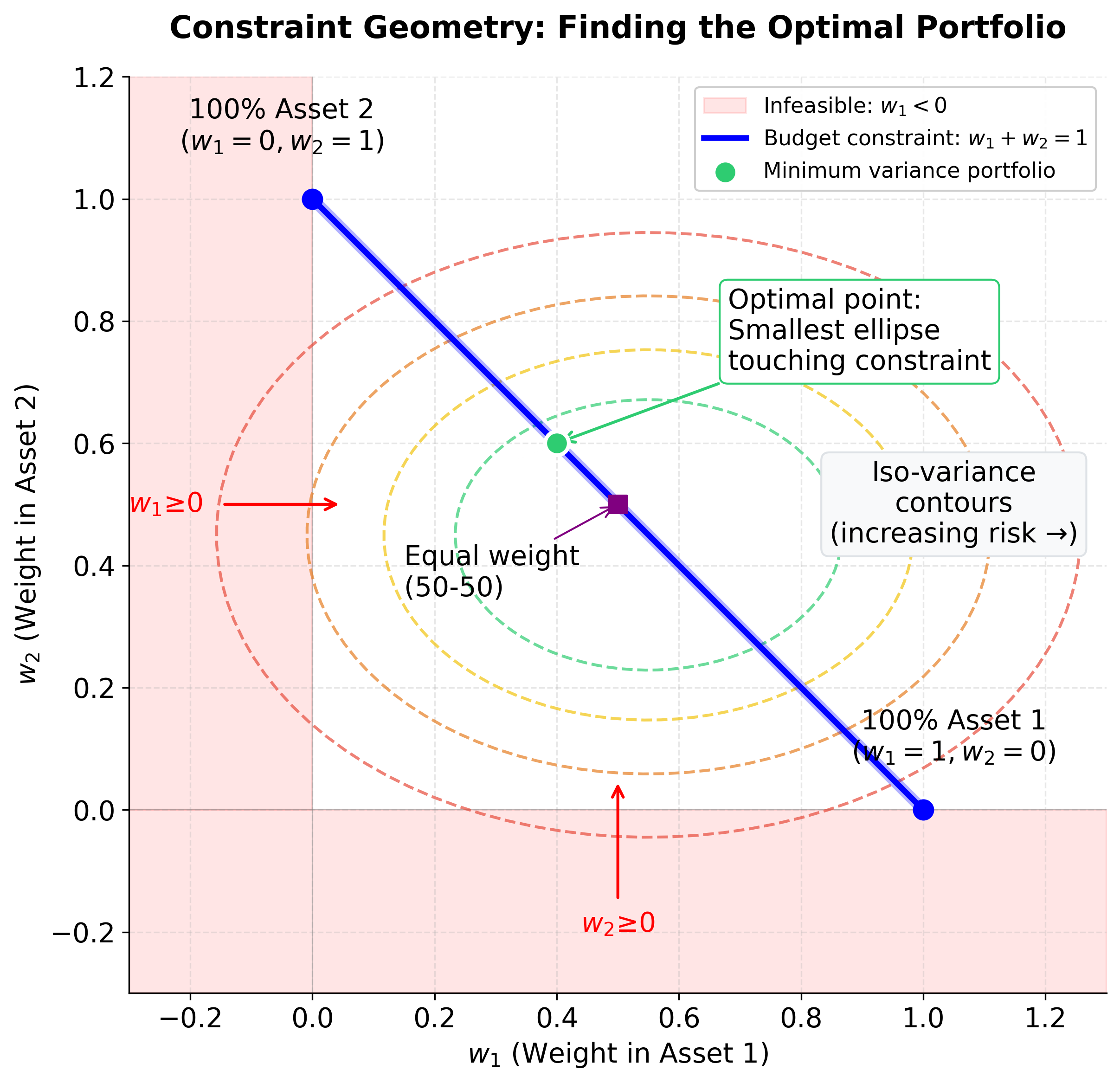
• Budget constraint ($\sum_{i=1}^{n} w_i = 1$): Ensures we invest exactly 100% of our available capital, no more and no less. This prevents the optimizer from suggesting we hold cash or borrow money (unless we explicitly allow it). The constraint can be written in matrix form as $\mathbf{1}^T w = 1$, where $\mathbf{1}$ is a vector of ones.

• Return constraint ($\sum_{i=1}^{n} w_i \mu_i = \mu_{target}$): Ensures our portfolio achieves a specific expected return target $\mu_{target}$. In matrix form, this is $w^T \mu = \mu_{target}$. By varying $\mu_{target}$, we can trace out the efficient frontier, which is the set of portfolios that offer the best risk-return trade-off.

• Non-negativity constraints ($w_i \geq 0$ for all $i \in \{1, 2, \ldots, n\}$): Prevents short selling (negative weights). In practice, many investors cannot or prefer not to short sell, so this constraint reflects real-world limitations. If we remove this constraint, we allow short selling, which can lead to more aggressive portfolios.

Mathematical Properties: Why This Problem is Well-BehavedLink Copied

The quadratic programming formulation for portfolio optimization has several important mathematical properties that make it both theoretically sound and practically solvable:

Convexity: The Guarantee of Global Optimality

The objective function $w^T \Sigma w$ is convex when the covariance matrix $\Sigma$ is positive semi-definite, which is always true for valid covariance matrices. This convexity property guarantees that:

• Any local minimum is also a global minimum, so we can't get "stuck" in a suboptimal solution
• The optimization problem is well-behaved and can be solved efficiently
• The solution is unique (or the set of optimal solutions is convex)

This convexity makes portfolio optimization computationally tractable: we're not dealing with a complex non-convex landscape with many local minima, but rather a smooth, bowl-shaped function with a single optimal solution.

The Quadratic Nature: Capturing Non-Linear Risk

The quadratic form $w^T \Sigma w$ captures the essential non-linearity of portfolio risk. Unlike expected returns (which combine linearly), risk grows quadratically with position sizes. This means:

• Doubling your position in an asset quadruples its contribution to portfolio variance
• The cross-terms (covariances) create complex interactions that linear models cannot represent
• Diversification benefits emerge naturally from the mathematical structure

This quadratic relationship is why simple linear approaches fail for portfolio optimization. The problem fundamentally requires a quadratic framework to capture the true nature of portfolio risk.

Visualizing Portfolio OptimizationLink Copied

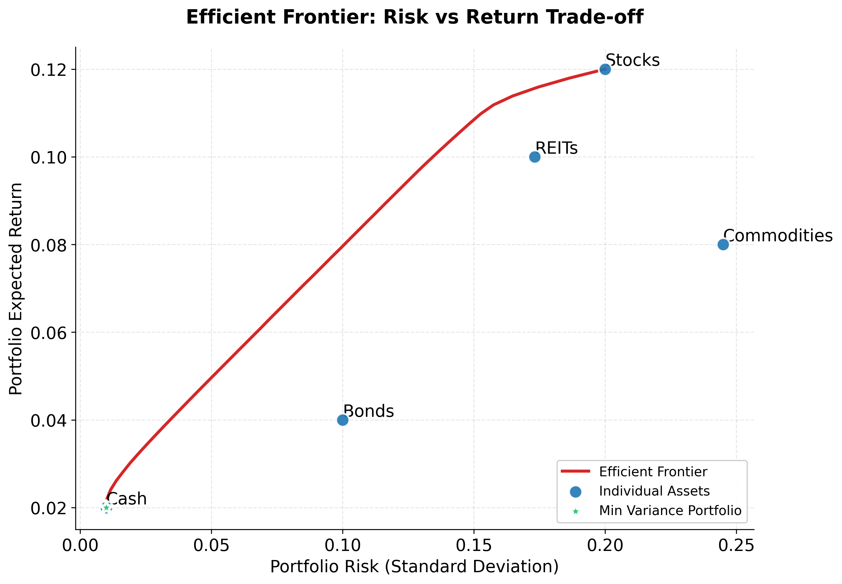
With the mathematical framework in place, let's see how these concepts manifest with real asset data. We'll construct a five-asset portfolio and visualize the efficient frontier, the set of optimal portfolios that offer the highest return for each level of risk.

Now let's visualize the efficient frontier by solving the optimization problem for different target returns:

ExampleLink Copied

A Concrete Walkthrough: From Data to Optimal PortfolioLink Copied

The efficient frontier visualization shows us what optimal portfolios look like, but how do we actually find them? In this section, we'll work through the complete mathematical derivation for the minimum variance portfolio, solving the optimization problem by hand using Lagrange multipliers. This walkthrough reveals the structure underlying portfolio optimization and shows exactly how the covariance matrix determines optimal allocations.

Setting Up the Problem: Our Five Assets

Suppose we're constructing a portfolio from five asset classes, each with distinct risk-return characteristics:

Expected Returns (annualized):

• Stocks: 12% (highest return, highest risk)
• Bonds: 4% (low return, low risk)
• Commodities: 8% (moderate return, high volatility)
• REITs: 10% (good return, moderate risk)
• Cash: 2% (lowest return, essentially no risk)

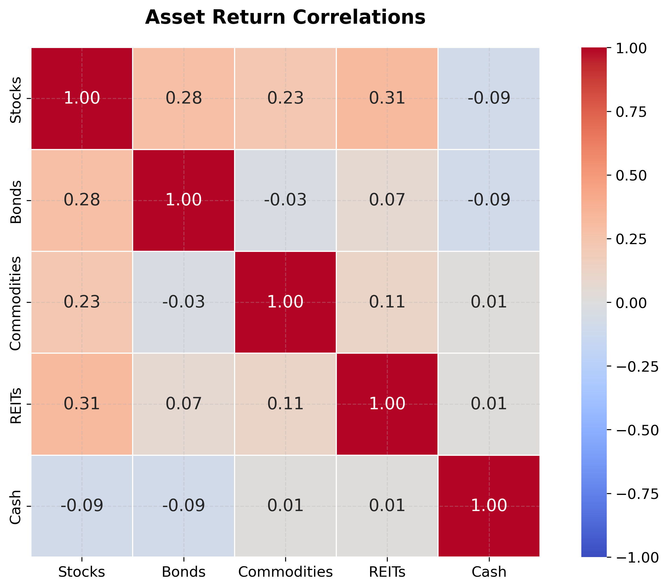
Covariance Matrix (annualized):

Let's interpret what this covariance matrix tells us:

• Diagonal elements (variances): The diagonal elements $\Sigma_{ii} = \sigma_i^2$ represent individual asset variances. For example:

  • Stocks: $\sigma_{\text{Stocks}}^2 = 0.04 \Rightarrow \sigma_{\text{Stocks}} = \sqrt{0.04} = 0.20$ (20% volatility)
  • Commodities: $\sigma_{\text{Commodities}}^2 = 0.06 \Rightarrow \sigma_{\text{Commodities}} = \sqrt{0.06} \approx 0.245$ (24.5% volatility)
  • Cash: $\sigma_{\text{Cash}}^2 \approx 0$ (essentially risk-free)

• Off-diagonal elements (covariances): The off-diagonal elements $\Sigma_{ij} = \sigma_{ij}$ (for $i \neq j$) measure how asset returns move together:

  • Stocks-Bonds: $\sigma_{\text{Stocks,Bonds}} = 0.01 > 0$ (tend to move together)
  • Commodities-Bonds: $\sigma_{\text{Commodities,Bonds}} = 0$ (uncorrelated, offering diversification potential)

Our Goal: Finding the Minimum Variance Portfolio

The minimum variance portfolio is the portfolio with the lowest possible risk (variance) that still satisfies our constraints. This represents the leftmost point on the efficient frontier, which is the safest possible portfolio we can construct from these assets.

Step 1: Setting Up the Optimization Problem

For the minimum variance portfolio, we want to minimize portfolio variance subject to our constraints:

subject to:

Notice we don't have a return constraint here. We're purely minimizing risk. This gives us the absolute minimum risk portfolio, which we can then use as a starting point for constructing portfolios with higher returns.

Step 2: Understanding the Gradient

To solve this optimization problem, we need to find where the gradient (slope) of our objective function equals zero. The gradient tells us the direction of steepest increase, so setting it to zero finds the minimum.

The gradient of $\frac{1}{2} w^T \Sigma w$ with respect to $w$ is:

This makes intuitive sense: the gradient is a linear function of the weights, where each component tells us how sensitive the portfolio variance is to changes in each asset's weight.

Step 3: Using Lagrange Multipliers to Handle Constraints

Since we have a constraint (weights must sum to 1), we use the method of Lagrange multipliers. This technique converts our constrained optimization problem into an unconstrained one by introducing a Lagrange multiplier $\lambda$.

We form the Lagrangian:

where:

• $L(w, \lambda)$: The Lagrangian function, which combines the objective function and the constraint
• $w$: The vector of portfolio weights (decision variables)
• $\lambda$: The Lagrange multiplier (also a decision variable to be determined)
• $\frac{1}{2} w^T \Sigma w$: The original objective function (portfolio variance)
• $\sum_{i=1}^{5} w_i - 1 = 0$: The budget constraint written in standard form

The second term penalizes solutions that violate our constraint. The multiplier $\lambda$ will be determined as part of the solution and represents the "shadow price" of the constraint, which is how much the objective function would improve if we relaxed the constraint by one unit.

Step 4: Finding the Optimality Conditions

Taking partial derivatives and setting them to zero gives us the optimality conditions (first-order necessary conditions for optimality):

where:

• $\frac{\partial L}{\partial w}$: The gradient of the Lagrangian with respect to $w$ (a vector)
• $\frac{\partial L}{\partial \lambda}$: The partial derivative of the Lagrangian with respect to $\lambda$ (a scalar)
• $\mathbf{1}$: A $5 \times 1$ vector of ones: $\mathbf{1} = [1, 1, 1, 1, 1]^T$
• $\mathbf{0}$: A $5 \times 1$ vector of zeros

Rearranging, we get the system of equations:

The first equation tells us that at the optimum, the gradient $\Sigma w$ must be proportional to the vector of ones. The second equation enforces our budget constraint.

Step 5: Deriving the Closed-Form Solution

From the first optimality condition $\Sigma w = \lambda \mathbf{1}$, we can solve for $w$ by left-multiplying both sides by $\Sigma^{-1}$ (assuming $\Sigma$ is invertible, which is true for positive definite covariance matrices):

Since $\Sigma^{-1} \Sigma = I$ (the identity matrix), we get:

This tells us the optimal weights are proportional to $\Sigma^{-1} \mathbf{1}$, which is the inverse covariance matrix times a vector of ones. The inverse covariance matrix appears because we're essentially "dividing out" the covariance structure to find the optimal allocation.

Substituting this expression for $w$ into the budget constraint $\mathbf{1}^T w = 1$:

Since $\lambda$ is a scalar, we can factor it out:

Solving for $\lambda$:

Note that $\mathbf{1}^T \Sigma^{-1} \mathbf{1}$ is a scalar: it equals the sum of all elements in $\Sigma^{-1}$. This scalar is always positive for positive definite covariance matrices.

Substituting this value of $\lambda$ back into $w = \lambda \Sigma^{-1} \mathbf{1}$, we get the optimal weights:

where:

• $w^*$: The optimal portfolio weights (an $n \times 1$ vector)
• $\Sigma^{-1}$: The inverse of the covariance matrix (an $n \times n$ matrix)
• $\mathbf{1}$: A vector of ones (an $n \times 1$ vector)
• $\mathbf{1}^T \Sigma^{-1} \mathbf{1}$: A scalar equal to the sum of all elements in $\Sigma^{-1}$

What This Solution Tells Us

This closed-form solution shows that the minimum variance portfolio weights are determined entirely by the covariance structure, not by expected returns. The solution is proportional to the inverse of the covariance matrix, scaled so the weights sum to one.

The denominator $\mathbf{1}^T \Sigma^{-1} \mathbf{1}$ is a normalization constant that ensures our weights sum to 1. The numerator $\Sigma^{-1} \mathbf{1}$ tells us the "raw" optimal allocation before normalization.

This solution has several advantages:

• It's analytical: we can compute it directly without iterative optimization.
• It's unique: the convexity of the problem guarantees a single optimal solution.
• It's interpretable: the inverse covariance matrix captures how assets should be weighted to minimize risk.

In practice, we would compute this using numerical linear algebra (solving the system of equations rather than explicitly inverting the matrix), but this closed-form expression gives us deep insight into the mathematical structure of the problem.

ImplementationLink Copied

While the closed-form solution provides insight into the mathematical structure, practical portfolio optimization requires numerical methods that can handle additional constraints like no-short-selling requirements. We'll implement portfolio optimization using scipy's optimization tools, translating the mathematical formulation directly into code.

Setting Up the Optimization FunctionLink Copied

First, we'll create a function that sets up and solves the portfolio optimization problem. This function takes expected returns, a covariance matrix, and an optional target return as inputs.

Finding the Minimum Variance PortfolioLink Copied

Let's optimize for the minimum variance portfolio, which represents the lowest-risk allocation possible given our assets.

The minimum variance portfolio concentrates in low-volatility assets, primarily Cash and Bonds, while avoiding high-volatility assets like Commodities. This allocation achieves the lowest possible portfolio risk given the available assets. The expected return is modest (typically 2-4% for this asset mix), reflecting the conservative nature of pure risk minimization. A Sharpe ratio above 0.5 indicates reasonable risk-adjusted performance; values above 1.0 are considered strong.

Optimizing for a Target ReturnLink Copied

Now let's optimize for a specific target return of 8% to see how the optimal allocation changes when we require higher returns.

To achieve 8% expected return, the optimizer shifts weight toward Stocks and REITs while reducing Cash and Bonds. The resulting portfolio risk increases substantially. Compare this to the minimum variance portfolio to see the risk cost of higher returns. If the Sharpe ratio improves (or remains similar), the additional return justifies the extra risk. If it decreases significantly, consider whether the target return is realistic given the available assets.

Comparing PortfoliosLink Copied

Let's compare the minimum variance portfolio with the target return portfolio to see the trade-offs.

This comparison illustrates the efficient frontier trade-off. Moving from minimum variance to an 8% target return increases portfolio risk by roughly 2-3x, a significant jump for a 4-5 percentage point return increase. The Sharpe ratios indicate whether this trade-off is favorable: if both portfolios have similar Sharpe ratios, the choice depends purely on risk tolerance. If the target portfolio has a lower Sharpe ratio, the additional return may not justify the extra risk.

Alternative Implementation: Custom QP SolverLink Copied

To connect our theoretical derivation with code, let's implement the Lagrange multiplier solution from the Example section. This solver directly constructs and solves the KKT system we derived earlier:

The custom solver produces the same weights as scipy's numerical optimizer (difference < $10^{-6}$), confirming both methods solve the same mathematical problem correctly. The analytical approach is faster for small portfolios without inequality constraints, while scipy's SLSQP handles no-short-selling bounds and other inequality constraints that the closed-form solution cannot accommodate.

Key ParametersLink Copied

Below are the main parameters that affect how portfolio optimization works and performs.

• expected_returns: Array of annualized expected returns for each asset. Estimate from historical means or factor models. Errors in return estimates significantly impact optimal weights, so consider using shrinkage toward the grand mean or focusing on minimum variance (which ignores returns).

• cov_matrix: Annualized covariance matrix of asset returns. Must be positive semi-definite. Use sklearn.covariance.LedoitWolf for shrinkage estimation when assets-to-observations ratio exceeds 0.3. Sample covariances are unreliable when this ratio exceeds 0.5.

• target_return: Target annualized return for the portfolio. Must be between min and max individual asset returns to be feasible. Set to None for minimum variance portfolio. Start with conservative targets (e.g., 2-3% above minimum variance return) to avoid extreme allocations.

• bounds: Weight constraints per asset, typically (0, 1) to prevent short selling. Use (0, 0.3) to cap any single position at 30%. Set (-0.3, 1) to allow limited short selling. More restrictive bounds reduce optimization benefit but improve robustness.

• method: Optimization algorithm. Use 'SLSQP' (default) for most problems since it handles equality and inequality constraints efficiently. Use 'trust-constr' for very large problems (500+ assets) or when SLSQP fails to converge.

• constraints: List of constraint dictionaries with 'type' ('eq' for equality, 'ineq' for inequality) and 'fun' (function returning 0 when satisfied for eq, or ≥0 for ineq). The budget constraint sum(w) = 1 should be included in all portfolio optimization problems.

Key MethodsLink Copied

The following are the most commonly used methods for portfolio optimization.

• optimize_portfolio(expected_returns, cov_matrix, target_return=None): Main wrapper function defined above. Returns optimal weights as a numpy array. Use target_return=None for minimum variance; specify a float (e.g., 0.08 for 8%) for target return optimization.

• scipy.optimize.minimize(objective, x0, method, bounds, constraints): Core scipy function. The objective computes portfolio variance ($w^T \Sigma w$), x0 is the initial guess (equal weights work well), bounds constrain individual weights, and constraints enforce budget and return requirements. Check result.success to verify convergence.

Practical ApplicationsLink Copied

Practical ImplicationsLink Copied

Quadratic programming for portfolio optimization works well when balancing risk and return across liquid assets with sufficient historical data. The approach is particularly effective for traditional asset allocation involving stocks, bonds, and other securities where covariance relationships remain reasonably stable over time. Institutional investors managing portfolios of 50-500 assets with 3+ years of daily data typically see the strongest benefits.

The linear constraint structure makes QP well-suited for institutional settings with regulatory requirements, sector limits, or concentration restrictions. Common constraints include maximum sector allocations (e.g., no more than 25% in technology), minimum liquidity requirements, and ESG restrictions. For individual investors, QP provides a systematic framework for constructing diversified portfolios aligned with specific risk tolerance levels.

QP may be less appropriate for illiquid assets, assets with limited historical data (fewer than 60 monthly observations), or situations where return distributions exhibit significant fat tails or regime changes. In these cases, robust optimization, scenario-based approaches, or risk parity methods often perform better. The choice depends on data availability, the stability of asset relationships, and whether mean-variance optimization captures the investor's true objectives.

Best PracticesLink Copied

Use shrinkage estimators for the covariance matrix rather than raw sample covariances. The Ledoit-Wolf shrinkage estimator (sklearn.covariance.LedoitWolf) provides a data-driven shrinkage intensity that typically ranges from 0.1 to 0.5. When the ratio of assets to observations exceeds 0.5, consider structured estimators such as single-factor models or constant correlation models. These reduce estimation error and improve out-of-sample performance, particularly for larger portfolios.

Expected returns are notoriously difficult to estimate and often dominate portfolio optimization errors. Consider risk parity approaches that focus on risk allocation rather than return forecasting, or use the minimum variance portfolio (which ignores returns entirely). If return forecasts are required, combine multiple estimation methods (historical averages, factor models, analyst estimates) and shrink extreme forecasts toward the cross-sectional mean. Robust optimization techniques that explicitly model uncertainty in return estimates can also reduce sensitivity to estimation errors.

Incorporate transaction costs directly into the optimization by adding a penalty term proportional to portfolio turnover (typically 0.1-0.5% per unit of turnover for liquid equities). Include turnover constraints that limit total portfolio change per rebalancing period to 10-30% to prevent excessive trading. Rebalance monthly or quarterly depending on transaction costs and volatility. More frequent rebalancing captures opportunities but incurs higher costs. Validate results using out-of-sample backtesting over multiple market regimes before deployment.

Data Requirements and PreprocessingLink Copied

Portfolio optimization requires historical return data for all candidate assets. For stable covariance estimates, use at least 60 monthly observations (5 years) or 252 daily observations (1 year), with longer windows preferred when available. The ratio of observations to assets should exceed 2:1 to avoid singular covariance matrices. For a 100-asset portfolio, aim for at least 200 observations. Daily data provides more observations but may introduce noise from microstructure effects; weekly returns often balance these concerns.

Annualize returns and covariances consistently: multiply daily returns by 252 (or weekly by 52), and multiply daily covariances by 252. Ensure return data is adjusted for stock splits, dividends, and other corporate actions. Handle missing data by either excluding assets with gaps or using interpolation, but recognize that extensive imputation can distort covariance estimates. For international assets, align time zones and handle currency effects explicitly.

The covariance matrix must be positive semi-definite for the optimization to have a solution. Sample covariance matrices are positive definite when observations exceed assets, but near-singular matrices can occur with highly correlated assets or redundant securities. If the solver reports numerical issues, add a small regularization term to the diagonal (e.g., $10^{-6}$ times the identity matrix) or remove highly correlated asset pairs. Do not standardize returns for portfolio optimization. Work with raw returns and covariances to preserve the economic interpretation of volatility and correlation.

Common PitfallsLink Copied

The most significant error is "error maximization," where optimization algorithms exploit estimation noise, overweighting assets with spuriously high returns or low covariances. This produces unstable portfolios with extreme positions that reverse when estimates are updated. The problem worsens as the ratio of assets to observations increases. Mitigation requires shrinkage estimators, position limits, or robust optimization techniques that account for parameter uncertainty.

Ignoring transaction costs leads to portfolios that look optimal on paper but underperform after trading expenses. Without cost penalties, optimizers suggest frequent small adjustments that erode returns through bid-ask spreads and market impact. Similarly, omitting practical constraints (minimum position sizes of $10,000+, sector limits, liquidity requirements) produces portfolios that cannot be implemented. Include realistic constraints from the start, as adding them later significantly changes optimal allocations.

Overfitting to historical data causes portfolios that perform well in backtests but poorly in live trading. This risk increases with shorter estimation windows, more assets, or frequent optimization. Use at least 3-5 years of data for estimation, validate with out-of-sample backtests across different market regimes, and be skeptical of Sharpe ratios above 1.5 in backtests. These often reflect data mining rather than genuine alpha. Limit optimization frequency to monthly or quarterly to avoid reacting to noise.

Computational ConsiderationsLink Copied

Portfolio QP problems are computationally tractable for most practical applications. For portfolios under 500 assets, scipy's minimize with method='SLSQP' solves in under 100ms. CVXPY with the OSQP or ECOS solver handles up to 2,000 assets efficiently. Commercial solvers like Gurobi or MOSEK scale to 10,000+ assets but require licenses. Memory scales as O(n²) for the covariance matrix. A 1,000-asset portfolio requires approximately 8MB for the covariance matrix alone.

For large universes (1,000+ assets), factor models reduce computational burden significantly. Representing the covariance matrix as $\Sigma = BFB^T + D$ where $B$ is an $n \times k$ factor loading matrix, $F$ is a $k \times k$ factor covariance matrix, and $D$ is a diagonal matrix of idiosyncratic variances reduces storage from O(n²) to O(nk). With $k = 10$-$50$ factors, this makes optimization feasible for universes of 5,000+ assets. The Barra and Axioma risk models are industry-standard examples.

When generating efficient frontiers or running sensitivity analysis, warm-start the solver with the previous solution to reduce iterations by 50-80%. For real-time applications requiring sub-second response, pre-compute efficient frontiers offline and interpolate. Parallelization helps for Monte Carlo simulations or optimizing multiple portfolios since each optimization is independent and scales linearly with available cores.

Performance and Deployment ConsiderationsLink Copied

Evaluate optimized portfolios using multiple metrics: Sharpe ratio for risk-adjusted returns, maximum drawdown for worst-case losses, and Sortino ratio for downside-focused assessment. Compare against benchmarks including equal-weight portfolios (a strong baseline), market-cap-weighted indices, and risk parity strategies. A minimum variance portfolio should achieve volatility 20-40% below an equal-weight portfolio; if the improvement is smaller, check for data or implementation issues.

Production systems require robust error handling. Catch solver failures from near-singular matrices or infeasible constraints and fall back to simpler solutions (e.g., equal-weight or previous optimal weights). Validate that output weights sum to 1.0 within tolerance ($10^{-6}$), satisfy all constraints, and contain no extreme positions (e.g., individual weights exceeding 30% unless explicitly allowed). Log all inputs and outputs for audit trails and debugging.

Establish monitoring thresholds for re-optimization: trigger updates when rolling correlations change by more than 0.15, when individual asset volatilities shift by more than 25%, or on a fixed schedule (monthly or quarterly). Avoid daily re-optimization, which amplifies estimation noise. Track realized versus predicted portfolio volatility. Persistent underestimation indicates covariance matrix problems. For regulatory compliance, maintain records of optimization parameters, constraints, and resulting allocations for at least 7 years.

SummaryLink Copied

Quadratic programming provides a mathematically sound and computationally efficient framework for portfolio optimization that has become the foundation of modern quantitative finance. By explicitly modeling the trade-off between risk and return through a quadratic objective function, QP allows investors to find optimal asset allocations that maximize risk-adjusted returns. The framework's flexibility in accommodating various constraints makes it suitable for a wide range of investment applications, from individual portfolio management to institutional asset allocation.

The key strength of the QP approach lies in its ability to capture the non-linear relationship between portfolio risk and asset weights, particularly the diversification benefits that arise from combining assets with different risk-return characteristics. The quadratic nature of the risk function naturally incorporates the covariance structure of asset returns, providing a systematic framework for portfolio construction that can improve in-sample risk-adjusted performance when inputs are accurately estimated.

However, the practical application of QP for portfolio optimization requires careful attention to data quality, model validation, and the incorporation of real-world constraints such as transaction costs and regulatory requirements. The sensitivity of optimal portfolios to input parameters necessitates robust estimation techniques and regular model validation to ensure continued effectiveness. When properly implemented with high-quality data and appropriate constraints, quadratic programming provides a powerful tool for constructing optimal investment portfolios that balance risk and return according to investor preferences and constraints.

QuizLink Copied

Ready to test your understanding? Take this quick quiz to reinforce what you've learned about quadratic programming for portfolio optimization.