

Master probability distributions essential for quantitative finance: normal, lognormal, binomial, Poisson, and fat-tailed distributions with Python examples.
Choose your expertise level to adjust how many terms are explained. Beginners see more tooltips, experts see fewer to maintain reading flow. Hover over underlined terms for instant definitions.
Common Probability Distributions in Finance
Probability distributions form the mathematical backbone of quantitative finance. Every time you estimate the risk of a portfolio, price an option, or model the likelihood of default, you are making assumptions about how random outcomes are distributed. These assumptions determine whether your models produce reasonable predictions or catastrophic failures.
The choice of distribution matters enormously. The 2008 financial crisis revealed that many risk models had dramatically underestimated the probability of extreme market moves. These models often assumed that returns followed a normal distribution, which assigns vanishingly small probabilities to the kind of large daily moves that occurred repeatedly during the crisis. Understanding the properties and limitations of different distributions has direct consequences for trading strategies, risk limits, and regulatory capital requirements.
This chapter covers the distributions you will encounter most frequently in quantitative finance: the normal distribution that underlies classical portfolio theory, the lognormal distribution that models asset prices, discrete distributions like the binomial and Poisson that appear in derivatives pricing and event modeling, and fat-tailed distributions that better capture the extreme events observed in real markets. For each distribution, we examine both the mathematical properties and the financial intuition behind its use.
The Normal Distribution
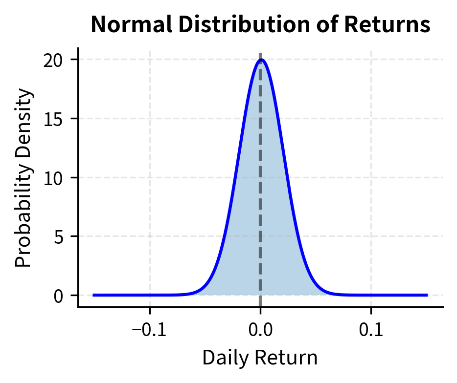
The normal distribution, also called the Gaussian distribution, is the starting point for most financial models. Its prominence stems from the Central Limit Theorem, which states that the sum of many independent random variables with finite variance tends toward a normal distribution regardless of the underlying distributions. Since asset returns can be viewed as the aggregate effect of many independent pieces of information hitting the market, the normal distribution provides a natural first approximation. This explains why the normal distribution became the default assumption in finance before computers made alternative distributions practical.
A continuous probability distribution characterized by its symmetric, bell-shaped curve. It is fully specified by two parameters: the mean (center) and variance (spread). Also known as the Gaussian distribution.
Mathematical Properties
To understand what it means for a random variable to follow a normal distribution, we must first grasp the concept of a probability density function. Unlike discrete random variables that take on specific values with certain probabilities, a continuous random variable like one following a normal distribution can take any value along the real line. The probability density function tells us how likely the variable is to fall in any particular region. The higher the density at a point, the more probable values near that point become.
A random variable follows a normal distribution with mean and variance , written , if its probability density function is:
Each component serves a specific purpose. Let's examine each component:
- : the value at which we evaluate the density
- : the mean (center of the distribution)
- : the standard deviation (controls the spread)
- : a normalization constant ensuring the density integrates to 1
- : measures how many standard deviations is from the mean, squared and scaled
The heart of the normal distribution lies in the exponential term. The quantity measures the squared distance between the point and the center of the distribution . Dividing by scales this distance relative to the spread of the distribution. A value two units away from the mean is much more unusual when than when , because the standardized distance is larger. The negative sign in the exponent ensures that the function decreases as we move away from the mean, and the exponential function transforms this squared distance into a probability density that decays smoothly and symmetrically.
The exponential of a negative quadratic creates the characteristic bell shape: values near the mean have high probability density, while values far from the mean have exponentially decreasing density. This rapid decay is why the normal distribution assigns negligible probability to extreme events. The probability of being more than a few standard deviations from the mean is vanishingly small, a property that proves problematic when modeling financial markets where extreme moves occur more frequently than this decay suggests. The quadratic term in the exponent is the key: because squaring grows faster than linear growth, and the exponential function amplifies this, the tails of the normal distribution thin out extraordinarily quickly.
The normalization constant deserves special attention. This factor ensures that when we integrate the density function over all possible values from negative infinity to positive infinity, we obtain exactly 1. This is the total probability. The arises from the Gaussian integral, one of the most famous results in calculus, while the in the denominator accounts for how wider distributions (larger ) must have lower peak heights to maintain the same total area under the curve.
Key parameters:
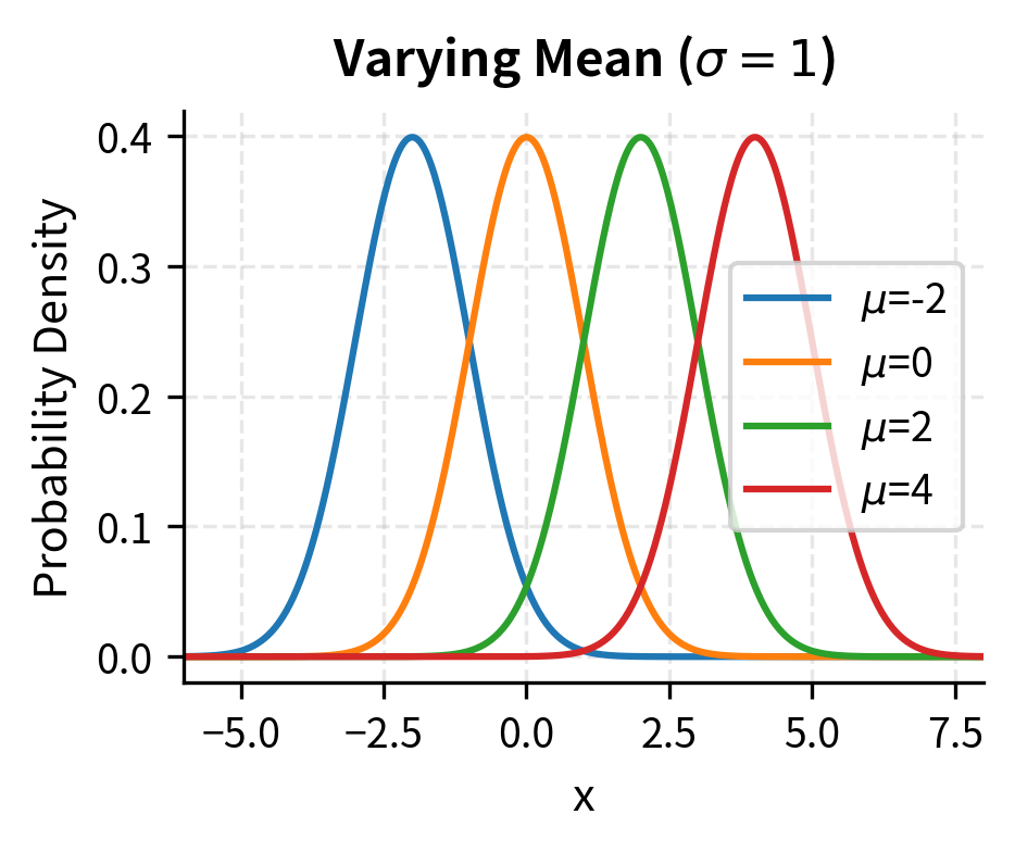
- Mean (): The center of the distribution and the expected value of . In finance, this represents the expected return.
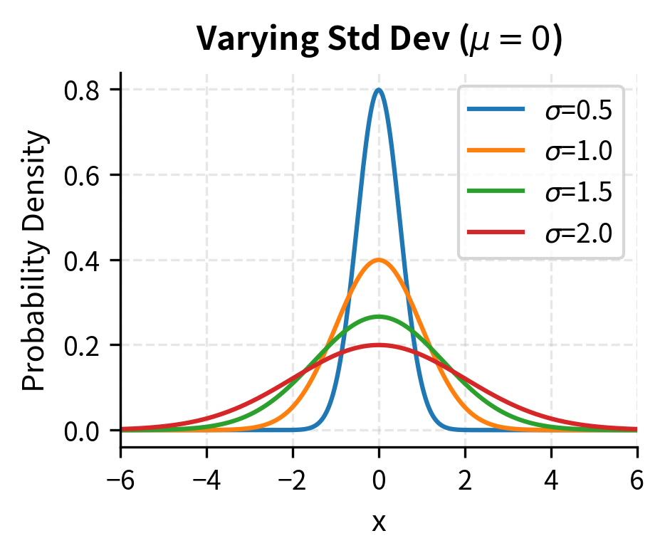
- Variance (): Measures the spread of the distribution. The square root, , is the standard deviation, which in finance we call volatility.
- Skewness: Zero for the normal distribution, meaning it is perfectly symmetric around the mean.
- Kurtosis: Equal to 3 for the normal distribution (or excess kurtosis of 0), which serves as the baseline for measuring tail thickness. Distributions with higher kurtosis have more probability mass in the tails and center, less in the shoulders.
The symmetry of the normal distribution is both its elegance and its limitation. A symmetric distribution treats upward and downward deviations identically, which aligns with our intuition that the laws of probability should not favor one direction over another for fundamental random processes. However, financial returns often exhibit asymmetry: crashes tend to be more severe and sudden than rallies of similar magnitude. This asymmetry, measured by skewness, is one reason the normal distribution serves as only a first approximation to market behavior.
The standard normal distribution is the special case where and . Any normal variable can be standardized:
This standardization process transforms any normal random variable into the canonical standard normal form. The operation first centers the distribution by subtracting the mean (so the new center is at zero), then scales it by dividing by the standard deviation (so the new spread equals one). This transformation preserves the essential shape of the distribution while placing it in a standard coordinate system.
This standardization is critical because it allows us to use a single table of probabilities for any normal distribution. The cumulative distribution function of the standard normal, denoted , gives the probability that a standard normal variable is less than . Before computers, statisticians relied on printed tables of values, and the standardization formula allowed them to answer questions about any normal distribution using this single reference. Even today, the standard normal serves as the universal reference point: when we speak of a "3-sigma event," we mean an outcome more than three standard deviations from the mean, regardless of what the actual mean and standard deviation are.
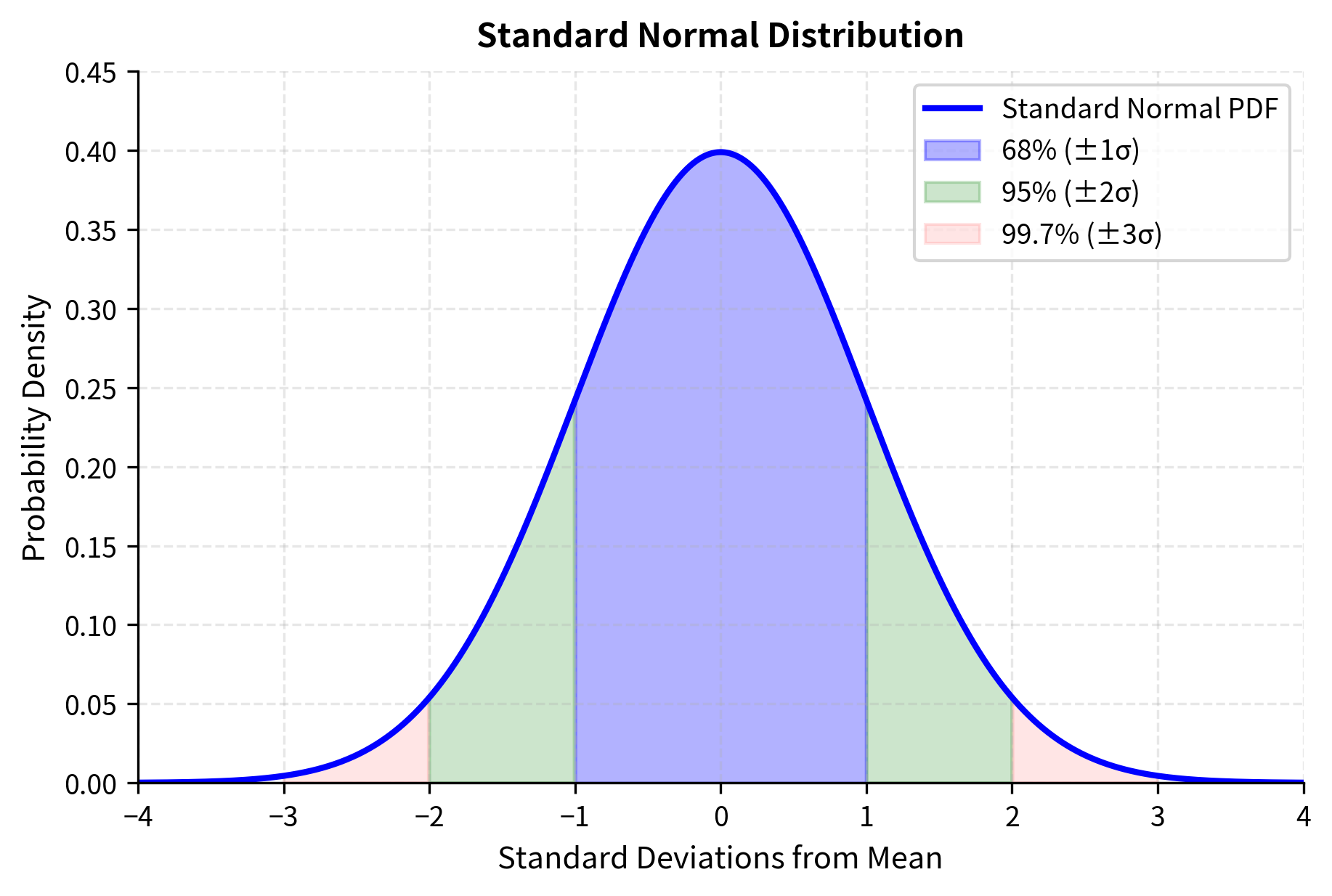
The 68-95-99.7 Rule
One of the most useful properties of the normal distribution is how probability mass is concentrated around the mean:
- Approximately 68% of observations fall within one standard deviation of the mean
- Approximately 95% fall within two standard deviations
- Approximately 99.7% fall within three standard deviations
These percentages emerge directly from integrating the normal density function, but their approximate values (68, 95, and 99.7) are worth committing to memory because they provide instant intuition for assessing how unusual any particular observation is. If someone tells you that an event was a "two-sigma move," you immediately know that such events occur roughly 5% of the time, or about one trading day in twenty.
This rule provides quick mental estimates for risk. If daily stock returns have a standard deviation of 1%, then under normality assumptions, you would expect a move larger than 3% (three standard deviations) to occur only about 0.3% of the time, or roughly once per year of trading days. This calculation reveals both the power and the danger of the normal assumption: it gives us precise quantitative predictions, but those predictions can be spectacularly wrong if the true distribution differs from normal.
Applications in Finance
The normal distribution appears throughout quantitative finance:
Portfolio theory assumes returns are normally distributed, which allows risk to be fully characterized by variance. Harry Markowitz's mean-variance optimization framework rests on this assumption. The profound insight behind this choice is that if returns are normal, then an investor who cares about expected utility needs to consider only the mean and variance of portfolio returns, since all higher moments are determined by these two parameters. This reduces the complex problem of choosing among thousands of possible portfolios to a tractable optimization problem with a clear geometric interpretation.
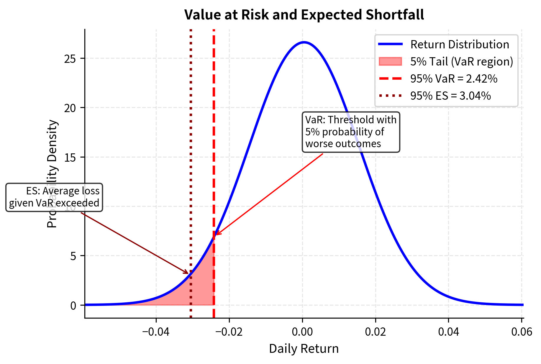
Value at Risk (VaR) calculations often assume normal returns. The VaR at confidence level (reported as a positive loss) is:
This formula translates the abstract concept of a tail quantile into a concrete loss estimate. Under the assumption that returns are normally distributed with mean and standard deviation , we seek the threshold such that returns fall below this level only percent of the time. The standard normal quantile tells us how many standard deviations below the mean this threshold lies.
Each component of this formula plays a specific role:
- : the Value at Risk at confidence level , representing the maximum expected loss
- : the expected return over the time horizon
- : the volatility (standard deviation of returns) over the time horizon
- : the -quantile of the standard normal distribution (e.g., for 95% confidence)
The formula works because under normality, the -percentile of returns is exactly . For example, the 95% VaR uses , meaning we expect losses to exceed this threshold only 5% of the time. Taking the negative of this return quantile yields the positive loss amount .
Option pricing via the Black-Scholes model assumes that log-returns are normally distributed, as we will explore in a later chapter.
These VaR figures tell us the maximum expected loss at each confidence level. The 1-day 95% VaR of approximately 2.4% means that under normal market conditions, we would expect to lose more than 2.4% only about one trading day in twenty. The 10-day VaR is higher due to the square-root-of-time scaling that arises from the assumption that daily returns are independent and identically distributed. This square-root relationship is a direct consequence of the variance addition property: if daily variances are , then the variance over days is , so the standard deviation scales as .
The Lognormal Distribution
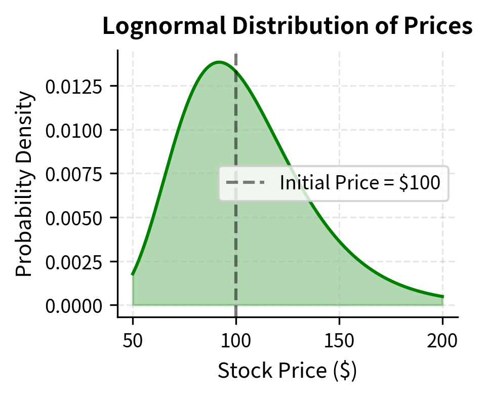
While returns may be approximately normal, prices cannot be. A stock price can rise 50% but cannot fall more than 100%. This asymmetry is captured by the lognormal distribution, which constrains values to be positive. The lognormal distribution emerges naturally when we consider the multiplicative nature of returns: a stock that gains 10% and then loses 10% does not return to its starting price. This multiplicative structure, when iterated over many periods, gives rise to the lognormal distribution through the magic of the exponential function.
A probability distribution of a random variable whose logarithm is normally distributed. If , then follows a lognormal distribution. Asset prices are often modeled as lognormal.
From Returns to Prices
The connection between normal returns and lognormal prices is one of the most important relationships in quantitative finance. If log-returns are normally distributed, then prices are lognormally distributed. Consider a stock with initial price and continuously compounded return over some period:
This equation captures a key relationship in how prices evolve. The exponential function converts the additive world of log-returns into the multiplicative world of price changes. When , the stock has grown by a factor of , or about 10.5%. The slight difference between the log-return and the percentage return becomes more pronounced for larger moves.
The components of this price equation are:
- : stock price at time
- : initial stock price
- : continuously compounded return over the period
- : the growth factor, converting log-return to price ratio
If , then follows a lognormal distribution. This relationship is fundamental: the exponential function transforms the symmetric, unbounded normal distribution into a right-skewed distribution bounded below by zero, which matches the behavior of asset prices that can rise without limit but cannot fall below zero. The transformation preserves the elegant properties of the normal distribution while mapping them onto the economically sensible domain of positive prices.
The probability density function of the lognormal distribution takes a form that reveals its connection to the normal:
Compare this to the normal density to see the key differences. The argument of the exponential now involves rather than , reflecting that we are measuring distance in the log-space. The presence of in front of the exponential arises from the chain rule when transforming from the normal to the lognormal through the change of variables.
Each element of this formula serves a distinct purpose:
- : the value at which we evaluate the density (must be positive)
- : the mean of , not the mean of itself
- : the standard deviation of , not of itself
- : this factor (compared to the normal PDF) accounts for the change of variables from to
The key insight is that and are parameters of the underlying normal distribution of log-values, not the lognormal variable itself. This distinction often causes confusion: when we say a stock has lognormal volatility of 20%, we mean the standard deviation of its log-returns, not of the returns themselves. The actual mean and variance of a lognormal variable are:
These formulas reveal how the parameters of the underlying normal distribution translate into the moments of the lognormal:
- : the expected value (mean) of the lognormal variable
- : the variance of
- : the mean of , the underlying normal distribution
- : the variance of
- : the mean is always greater than due to the convexity of the exponential function
The term in the mean formula is a convexity adjustment: because the exponential function is convex, Jensen's inequality tells us that for any non-constant random variable . Specifically, the curvature of the exponential means that high values of contribute disproportionately to the mean of . This is why the expected value of a lognormal variable is not simply but includes the variance correction, since higher variance increases this convexity effect. This seemingly technical point has profound practical implications: it means that an asset with higher volatility will have a higher expected price level even if the expected log-return remains unchanged.
Geometric Brownian Motion
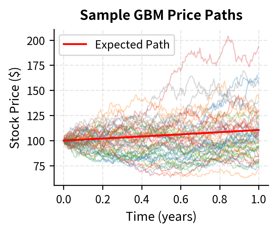
The standard model for stock price dynamics is geometric Brownian motion (GBM), which produces lognormally distributed prices. This model has been central to quantitative finance since Samuelson's work in the 1960s and forms the foundation for the Black-Scholes option pricing formula. Understanding GBM requires familiarity with stochastic calculus, but the core idea is intuitive. Prices evolve continuously with both a deterministic trend and random fluctuations proportional to the current price.
Under GBM, the stock price evolves according to:
This stochastic differential equation describes infinitesimal changes in the stock price. Each term has a clear interpretation:
- : infinitesimal change in stock price
- : current stock price
- : drift rate (expected return per unit time)
- : volatility (standard deviation of returns per unit time)
- : infinitesimal time increment
- : increment of a Wiener process (Brownian motion), with
The first term represents the deterministic trend, while the second term captures random fluctuations proportional to the current price. The key feature is that both terms are proportional to : a 10 stock with the same parameters will have the same percentage return distribution, but the absolute dollar changes will be ten times larger for the more expensive stock. This proportionality is what makes GBM appropriate for modeling asset prices, which tend to grow (or shrink) in percentage terms.
Solving this stochastic differential equation yields:
This solution tells us exactly where the stock price will be at any future time, given the realized path of the Brownian motion. The formula has a clear structure:
- : stock price at time
- : initial stock price at time 0
- : drift rate (annualized expected return)
- : volatility (annualized standard deviation)
- : time horizon in years
- : value of the Wiener process at time , with
- : Itô correction term arising from the quadratic variation of Brownian motion
The Itô correction appears because we apply Itô's lemma to : the second derivative term contributes to the drift. This correction is one of the key differences between ordinary calculus and stochastic calculus. In ordinary calculus, if we know , we would conclude that . However, when follows a diffusion process, the additional term arises from the non-zero quadratic variation of Brownian motion. This mathematical detail has important financial implications: it means the expected log-return is less than the expected arithmetic return, a difference that matters for long-horizon investing.
This model forms the foundation of the Black-Scholes option pricing formula.
Simulating Price Paths
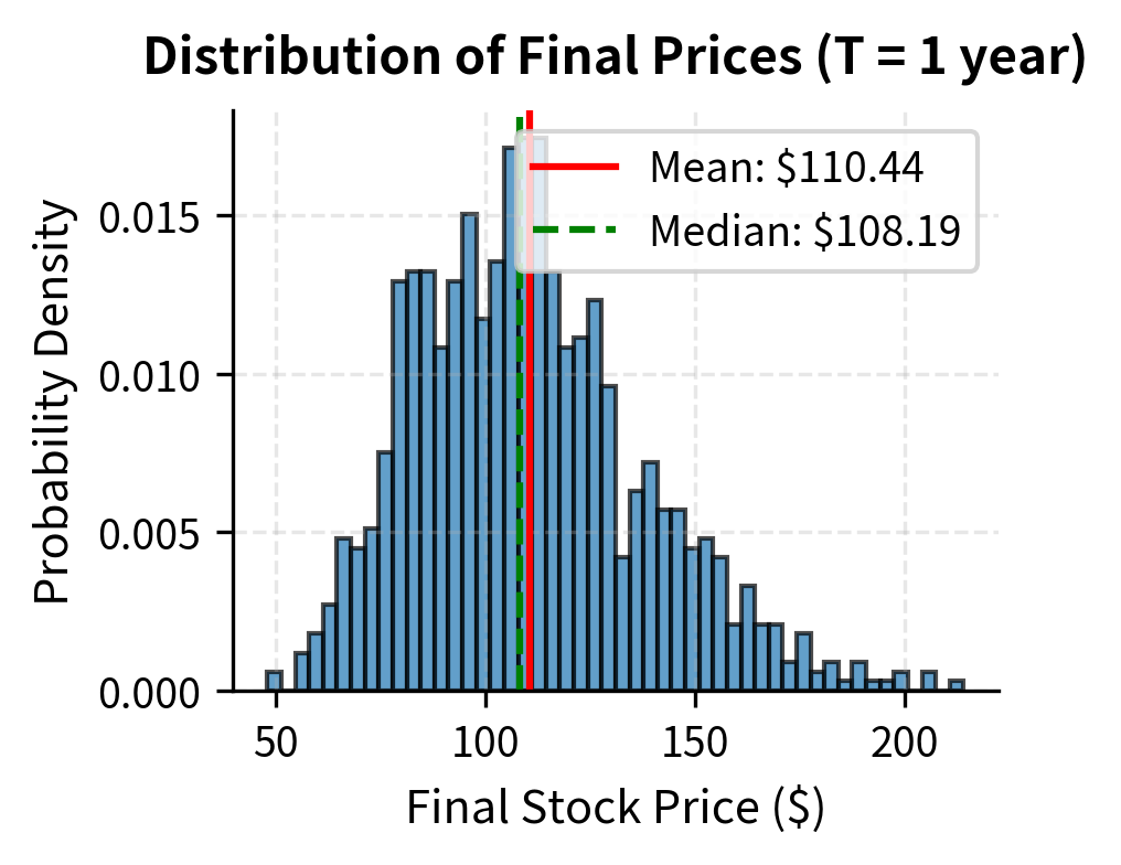
Monte Carlo simulation of stock prices under GBM is simple. We can either simulate the continuous process or use the exact solution. The approach below uses the exact solution, which is more efficient and avoids discretization errors that accumulate in step-by-step simulation methods. By using the closed-form solution for directly, we ensure that our simulated paths have the correct distribution regardless of the time step size.
Notice that the mean simulated price is close to the theoretical expected value of , but the median is lower. This is typical of lognormal distributions. Positive skewness means that a few very high outcomes pull the mean above the median. In practical terms, this means that while the average outcome is favorable, the most likely outcome (the mode) and the middle outcome (the median) are both lower than the average. An investor thinking about typical outcomes should focus on the median, while an investor thinking about long-run average performance should focus on the mean.
Discrete Distributions: Binomial and Poisson
Not all financial phenomena are continuous. Events like defaults, dividend announcements, or large jumps in prices are discrete occurrences. The binomial and Poisson distributions model these situations, providing a framework for counting how many times something happens rather than measuring continuous quantities. These distributions are particularly important in credit risk, where we count defaults in a portfolio, and in derivatives pricing, where discrete lattice models approximate continuous price processes.
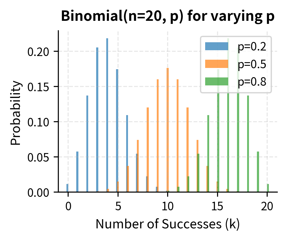
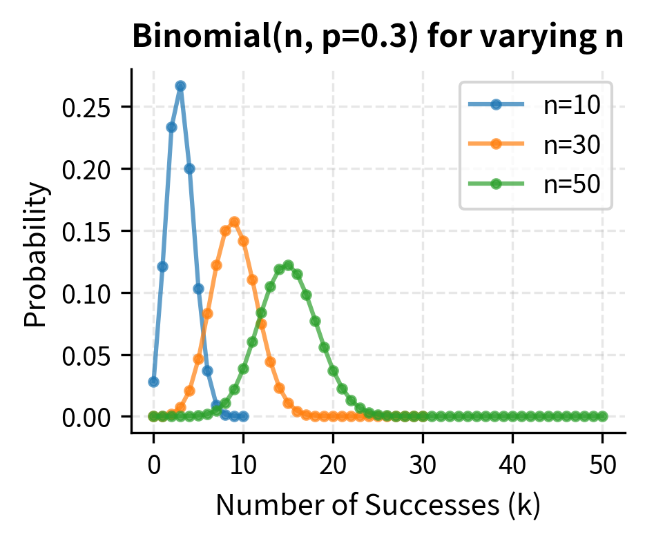
The Binomial Distribution
The binomial distribution models the number of successes in a fixed number of independent trials, each with the same probability of success. The classic example is flipping a coin multiple times and counting heads, but the same mathematics applies to questions such as: How many stocks in a portfolio will outperform? How many corporate bonds will default? How many days this month will have positive returns?
The probability distribution of the number of successes in independent Bernoulli trials, where each trial has success probability . Used in discrete option pricing models and credit risk modeling.
If , the probability mass function is:
This formula answers the question: if we have independent trials, each with success probability , what is the probability of getting exactly successes? The answer decomposes into two multiplicative components: the number of ways the successes can be arranged, and the probability of any particular arrangement.
Each component of this formula serves a specific purpose:
- : the number of successes we're computing the probability for
- : total number of independent trials
- : probability of success on each trial
- : the binomial coefficient, representing the number of ways to choose successes among trials
- : probability of exactly successes
- : probability of exactly failures
The formula multiplies the number of arrangements by the probability of each specific arrangement. Intuitively, if you flip a coin times with probability of heads, the PMF tells you the probability of getting exactly heads: you need successes (probability ), failures (probability ), and the binomial coefficient counts how many orderings produce that outcome. The key insight is that because the trials are independent, the probability of any specific sequence of outcomes is simply the product of the individual probabilities, and the binomial coefficient tells us how many such sequences lead to exactly successes.
The mean and variance have elegant formulas that reveal the distribution's structure:
These formulas encode intuitive relationships:
- : the expected number of successes
- : the variance in the number of successes
- : total number of trials
- : probability of success on each trial
- : probability of failure, which appears in variance because maximum variance occurs when (maximum uncertainty)
The expected number of successes, , is simply the number of trials times the success probability, exactly what intuition suggests. The variance formula is more subtle: it shows that variance is maximized when (complete uncertainty about each trial's outcome) and decreases toward zero as approaches 0 or 1 (near certainty). This makes sense because if is very close to 1, almost all trials succeed, leaving little room for variability in the total count.
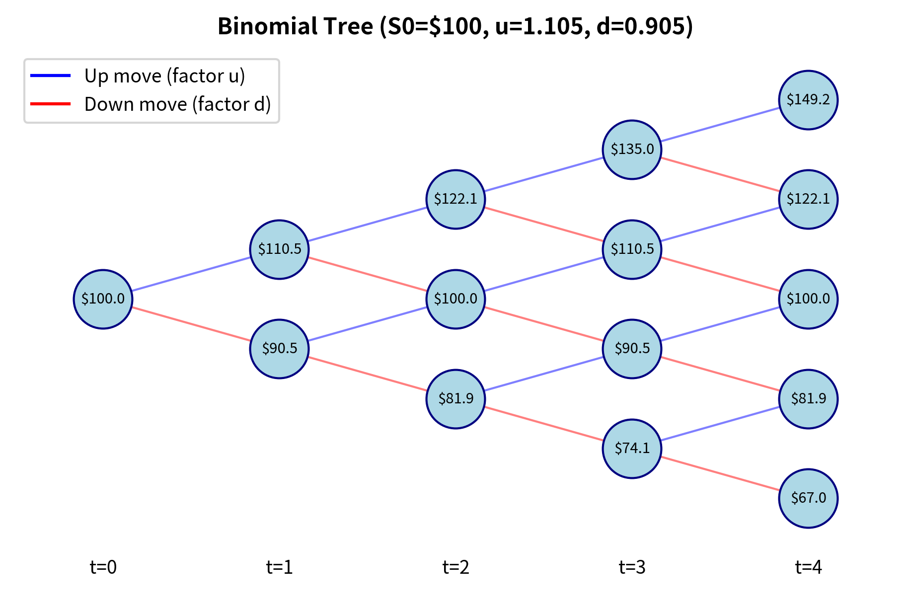
Binomial Option Pricing Model
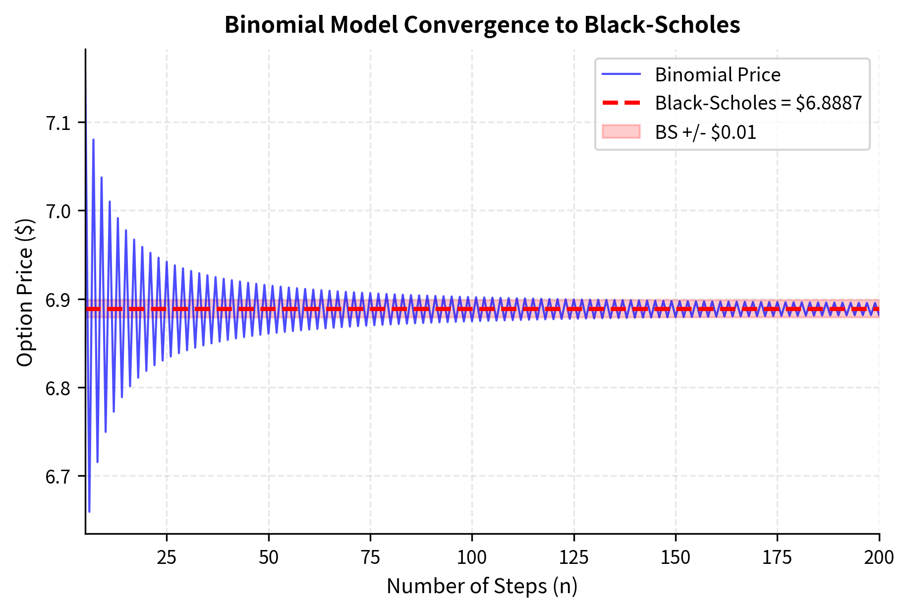
The Cox-Ross-Rubinstein (CRR) binomial model prices options by assuming that at each time step, the stock price either moves up by a factor or down by a factor . This discretization transforms the continuous option pricing problem into a tree of possible outcomes that can be analyzed one step at a time. While this may seem like a crude approximation to the continuous world of actual markets, the model provides deep insights into option pricing and converges to the continuous Black-Scholes formula as the number of time steps increases.
After steps, the stock price has experienced up moves and down moves, giving:
This formula shows how the final price depends entirely on the number of up moves, not their specific timing. The components are:
- : stock price at maturity after steps
- : initial stock price
- : up factor (price multiplier for an up move)
- : down factor (price multiplier for a down move)
- : number of up moves
- : number of down moves Whether the stock rises first and then falls, or falls first and then rises, the final price is the same as long as the total number of up and down moves matches. This path-independence is crucial for European options, which depend only on the final price, though it breaks down for path-dependent derivatives like Asian options.
The number of up moves follows a binomial distribution under the risk-neutral measure, with probability of an up move:
This risk-neutral probability is one of the most important concepts in derivatives pricing. Notice that is not the actual probability that the stock will go up. It is the artificial probability that makes the expected return on the stock equal to the risk-free rate. The components are:
- : risk-neutral probability of an up move
- : risk-free interest rate (annualized)
- : length of each time step in years
- : up factor (stock price multiplier for an up move)
- : down factor (stock price multiplier for a down move)
- : the growth factor for a risk-free investment over one time step
This formula is derived from the no-arbitrage condition: the expected stock return under the risk-neutral measure must equal the risk-free rate. Setting and solving for yields this result. The key insight is that option prices depend only on these risk-neutral probabilities, not on the actual probabilities of up and down moves. This separation of pricing from probability estimation is what makes derivatives pricing possible without knowing investors' risk preferences.
As the number of steps increases, the binomial model converges to the Black-Scholes price. This convergence illustrates how the discrete binomial model approximates the continuous-time lognormal model. The rate of convergence is roughly , meaning that doubling the number of steps roughly halves the error. This convergence is not merely a numerical curiosity; it reflects a deep mathematical connection between the binomial random walk and Brownian motion, formalized in Donsker's theorem.
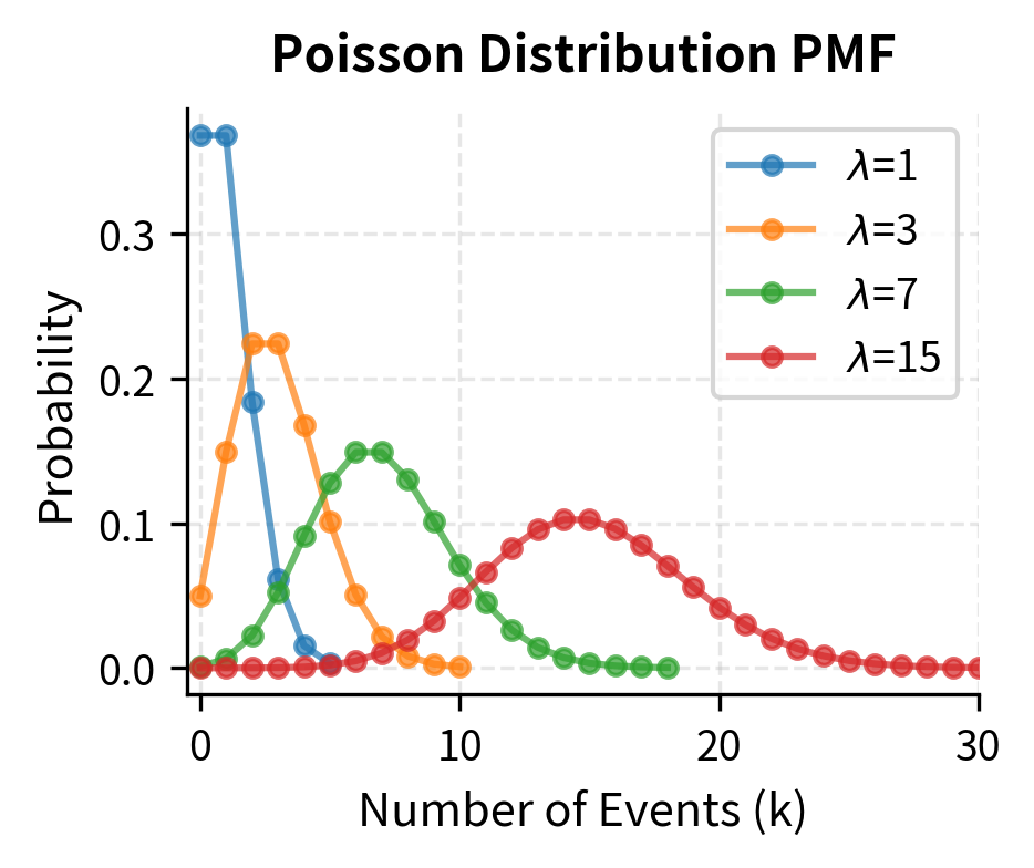
The Poisson Distribution
The Poisson distribution models the number of events occurring in a fixed interval when events happen at a constant average rate and independently of each other. Unlike the binomial distribution, which assumes a fixed number of trials, the Poisson distribution allows for any number of events, making it useful for modeling rare occurrences over a continuous interval.
A discrete probability distribution expressing the probability of a given number of events occurring in a fixed interval, when events occur at a constant average rate independently of each other. Used for modeling defaults, jumps, and arrival processes.
If , the probability mass function is:
This formula has a clear structure when we trace its derivation from first principles. Imagine dividing the interval into many tiny subintervals, each with a small probability of containing an event. As the number of subintervals goes to infinity while keeping the expected total number of events fixed at , we obtain the Poisson distribution.
The components of this formula are:
- : the number of events we're computing the probability for
- : the average rate of events (expected number of events in the interval)
- : the probability of zero events, which serves as a normalization factor
- : captures how the probability grows with more opportunities for events
- : accounts for the indistinguishability of event orderings
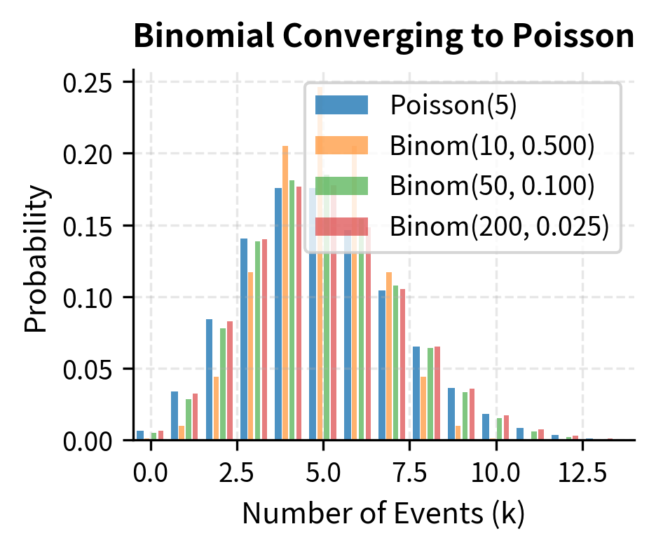
The Poisson distribution arises as the limit of a binomial distribution when and while remains constant, which corresponds to many trials with small individual probabilities. This limiting relationship explains why the Poisson distribution is appropriate for rare events: if we have many opportunities for something unlikely to happen, and the total expected count is finite, the number of occurrences follows a Poisson distribution. This is precisely the situation in credit risk (many bonds, each with a small default probability) and in jump modeling (many small time intervals, each with a small probability of containing a jump).
Both the mean and variance equal :
This property deserves emphasis:
- : the expected number of events
- : the variance in the number of events
- : the average rate parameter
The equality of mean and variance is a distinctive property of the Poisson distribution. When analyzing count data, if the observed variance significantly exceeds the mean (overdispersion), this suggests the Poisson model may be inadequate. Overdispersion often indicates that events are not independent. For instance, defaults may cluster in time due to common economic factors, or that price jumps tend to trigger subsequent jumps through market feedback effects.
Applications of the Poisson Distribution
The Poisson distribution is particularly useful for modeling:
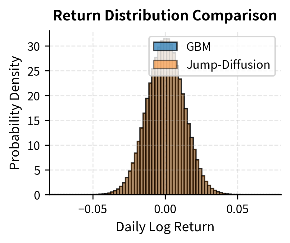
Jump processes in asset prices: The Merton jump-diffusion model adds Poisson-distributed jumps to geometric Brownian motion, capturing sudden large price movements that GBM alone cannot produce. In this model, the stock price follows GBM between jumps, but occasionally experiences discrete jumps whose arrival is governed by a Poisson process. This combination captures both the continuous fluctuations of normal trading and the occasional large movements caused by major news events.
Credit defaults in a portfolio: If defaults occur independently with a small probability, the number of defaults in a large portfolio is approximately Poisson distributed. This approximation underlies many credit risk models, although the assumption of independence often breaks down during systemic crises, when many borrowers default simultaneously.
Order arrivals: In market microstructure, the arrival of orders is often modeled as a Poisson process. This assumption implies that the time between consecutive orders follows an exponential distribution, without clustering or periodicity in order flow. While real markets show more complex arrival patterns, the Poisson model provides a useful baseline.
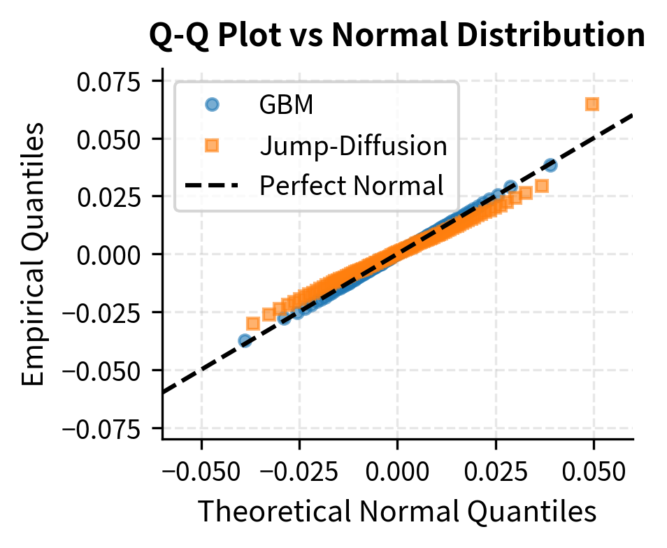
The jump-diffusion model produces returns with higher kurtosis (fatter tails) and more negative skewness than pure GBM. The minimum return is more extreme, reflecting occasional large negative jumps. These properties better match empirical observations of asset returns. The higher kurtosis indicates that the jump-diffusion model places more probability mass both in the center (small moves) and in the tails (large moves), with less probability in the intermediate range, exactly the pattern observed in real financial data.
Fat-Tailed Distributions
Empirical studies consistently show that asset returns have fatter tails than the normal distribution predicts. Events that should occur once in centuries under normality happen multiple times per decade. This observation has major implications for risk management. The discrepancy between theoretical and observed extreme event frequencies is not a minor technical issue. It represents a fundamental mismatch between the mathematical assumptions underlying most financial models and the actual behavior of markets.
Evidence of Fat Tails
The term "fat tails" refers to distributions where extreme events occur more frequently than a normal distribution would suggest. A distribution with fat tails places more probability mass in the regions far from the mean, meaning that large positive or negative values are more common than the normal distribution's rapid exponential decay would predict. Several ways to measure this phenomenon:
Kurtosis: The normal distribution has a kurtosis of 3 (or excess kurtosis of 0). Distributions with higher kurtosis have fatter tails. Equity returns typically exhibit excess kurtosis of 3 to 10, so extreme returns are far more common than the normal distribution predicts. The kurtosis measures the fourth moment of the distribution relative to its variance squared, essentially capturing how much probability mass resides in the tails versus the shoulders of the distribution.
Tail exponents: For very fat-tailed distributions, the probability of extreme events decays as a power law rather than exponentially. The tail exponent characterizes how fast this decay occurs. A smaller means slower decay and fatter tails, while larger means faster decay approaching the thin tails of the normal distribution.
The data reveals a stark departure from normality. Events beyond 4 standard deviations occur roughly 75 times more frequently than a normal distribution predicts. Under the normal assumption, a 5-sigma event should occur once every 7,000 years of trading, yet we observe multiple such events in just two decades. This massive discrepancy is not a statistical fluke. It reflects a fundamental difference between the mathematical properties of the normal distribution and the actual mechanics of how prices move in financial markets.
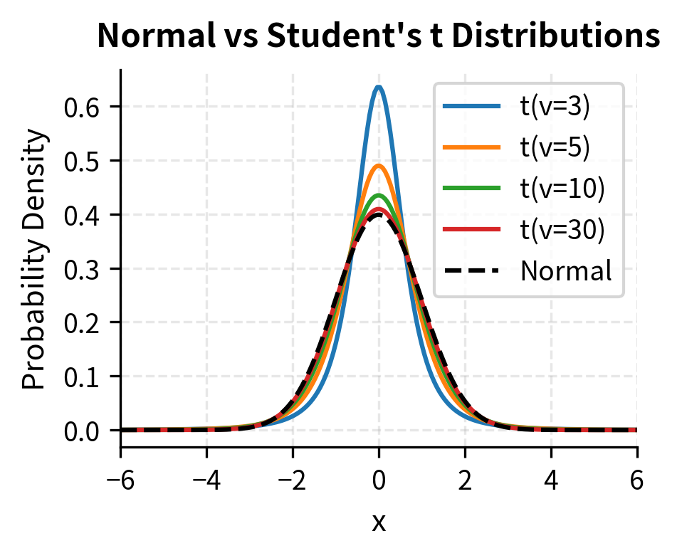
The Student's t Distribution
The Student's t distribution provides a simple way to model fat tails while retaining many convenient properties of the normal distribution. William Sealy Gosset originally developed the t distribution (writing under the pseudonym "Student") for quality control at Guinness brewery. It is now widely used in finance for modeling the heavy tails observed in return data.
A probability distribution with heavier tails than the normal distribution, characterized by its degrees of freedom parameter . As , it converges to the normal distribution. For small , it assigns higher probability to extreme events.
The probability density function of the standard t distribution with degrees of freedom is:
This formula may look complex, but its structure shows the key difference between the t distribution and the normal distribution. While the normal distribution uses the exponential function which decays very rapidly, the t distribution uses a power function which decays much more slowly. This slower decay is precisely what produces the heavier tails.
Each component:
- : the value at which we evaluate the density
- : degrees of freedom parameter (controls tail thickness; lower means fatter tails)
- : the gamma function, generalizing the factorial to non-integer values ( for positive integers)
- : a normalization constant ensuring the density integrates to 1
- : the core term that produces polynomial rather than exponential tail decay
The polynomial decay versus the normal's exponential decay is why the t distribution has heavier tails. To understand this intuitively, consider what happens as becomes large. For the normal distribution, decreases very fast. Doubling squares the exponent, making the probability essentially vanish. For the t distribution, doubling roughly halves the probability raised to a power, which is a much slower decay. As , the polynomial term converges to the exponential, and the t distribution approaches the normal.
Key properties of the t distribution:
- Degrees of freedom (): Controls tail thickness. Lower values mean fatter tails.
- Convergence: As , the t distribution approaches the standard normal.
- Variance: For , the variance is , which is always greater than 1. For , the variance is infinite. This is an extreme case where the tails are so heavy that second moments do not exist.
- Kurtosis: For , excess kurtosis is , always positive and decreasing in . For , the kurtosis is undefined because the fourth moment does not exist.
For financial applications, a t distribution with 4 to 6 degrees of freedom often fits return data well, capturing the observed excess kurtosis while staying manageable. The fact that empirically fitted degrees of freedom are typically in this range has important implications. With around 4, we are near the boundary where the fourth moment (and hence kurtosis) becomes undefined, indicating that we are dealing with genuinely heavy-tailed phenomena that push the limits of standard statistical tools.
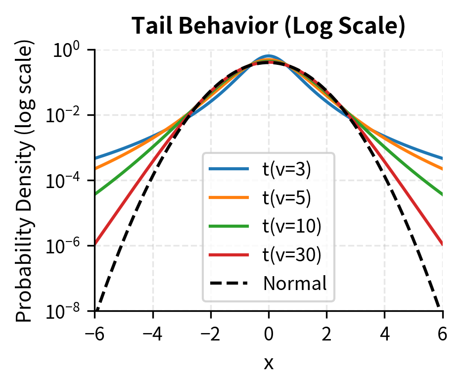
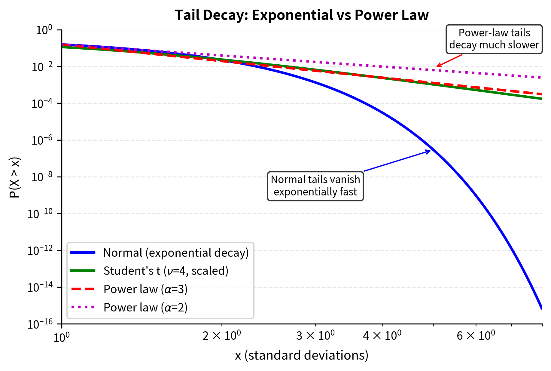
The log-scale plot on the right reveals how dramatically the distributions differ in their tails. At 5 standard deviations, the t distribution with 3 degrees of freedom assigns probability thousands of times higher than the normal distribution. This difference, while invisible on a linear scale where both probabilities appear to be essentially zero, has enormous practical significance for risk management. The one-sided probability of a 5-sigma event under a normal distribution is about 1 in 3.5 million; under a t distribution with 3 degrees of freedom scaled to have unit variance, it is about 1 in 600, a difference of several orders of magnitude that transforms a once-in-millennia event into something that can happen every few years.
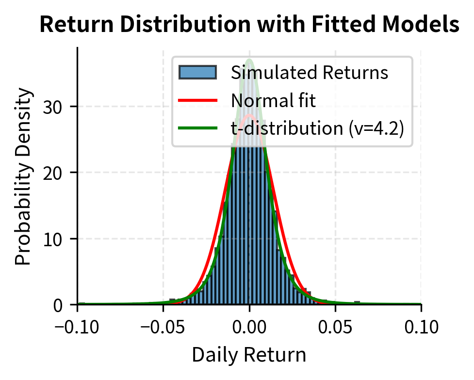
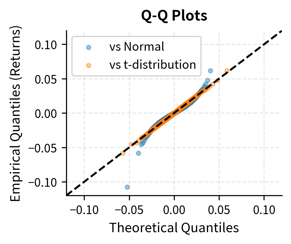
Fitting the t Distribution to Market Data
We can fit a scaled t distribution to observed returns and compare the fit to a normal distribution. This exercise demonstrates not just that the t distribution fits better, but quantifies how much better, providing a concrete measure of the inadequacy of the normal assumption.
The fitted t distribution has around 4-5 degrees of freedom, far from the normal limit. The large improvement in log-likelihood confirms that the t distribution better captures the observed return distribution. The log-likelihood difference of several thousand translates to overwhelming statistical evidence against the normal distribution. The odds ratio in favor of the t distribution is very large.
Power-Law Tails
Some financial time series have tails that are even fatter than what the t distribution can capture. In extreme cases, the tails follow a power law:
This asymptotic relationship describes the behavior of the survival function (the probability of exceeding a threshold) for large values. Unlike the exponential tails of the normal distribution or even the polynomial tails of the t distribution, power-law tails can be extraordinarily heavy, with profound implications for the existence of moments and the behavior of aggregates.
The components of this relationship are:
- : the probability that the random variable exceeds value (the survival function)
- : a large threshold value
- : the tail exponent (also called the tail index), which controls how fast probabilities decay
- : denotes asymptotic equivalence. The ratio of the two sides approaches a constant as
A larger means faster decay and thinner tails; a smaller means slower decay and fatter tails. The probability of extreme events decays polynomially rather than exponentially. For equity returns, empirical studies suggest for the tails, known as the "cubic law." Under this law, the probability of a return twice as large as a given threshold is approximately as likely. This is a much slower decay than the exponential falloff of normal distributions.
To appreciate the difference, consider that under a normal distribution, doubling the threshold from 4σ to 8σ reduces the probability by a factor of roughly , while under a cubic power law, the reduction is only a factor of 8. This staggering difference explains why normal-based risk models fail so spectacularly during market crises. They treat large moves as highly improbable when in fact they are merely uncommon.
A distribution where the probability of observing a value greater than decays as a power of : . The tail exponent determines how fat the tails are. Lower means fatter tails.
The implications of power-law tails are serious for risk management:
- Moments may not exist: If , the variance is infinite. If , even the mean is undefined. For the cubic law with , the variance exists but the fourth moment (kurtosis) does not, which explains why sample kurtosis estimates are so unstable.
- Slow convergence: The Central Limit Theorem converges very slowly for heavy-tailed distributions. While the theorem still applies (for ), the sample size needed for the normal approximation to become accurate can be impractically large.
- Tail risk dominates: With power-law tails, a small number of extreme events can dominate the total risk. In a portfolio context, this means that diversification benefits may be less than standard theory suggests.
Implications for Risk Management
Fat tails change how we should think about risk:
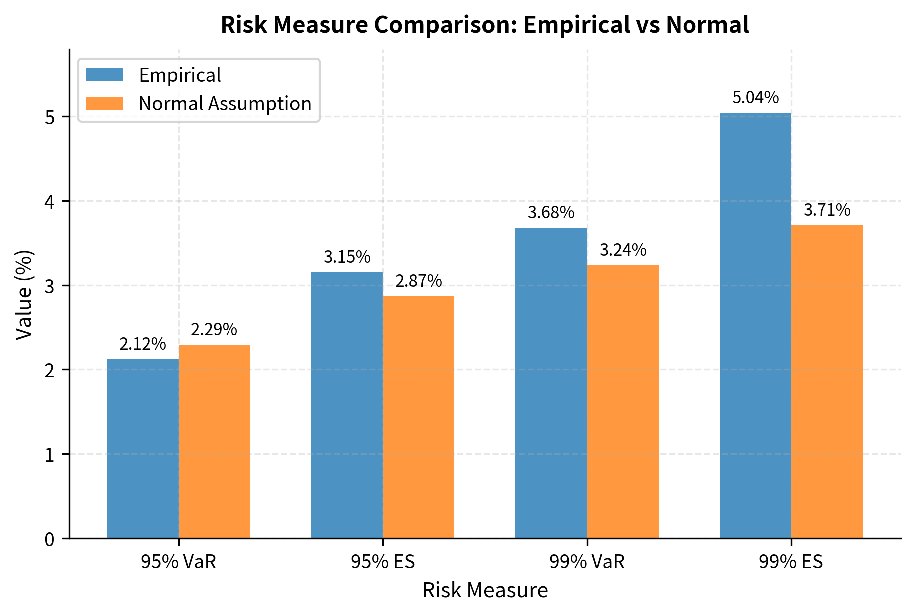
VaR underestimation: Using normal-based VaR systematically underestimates tail risk. The true 99% VaR may be two to three times larger than the normal approximation suggests. This systematic bias grows worse at higher confidence levels, precisely where accuracy matters most.
Expected shortfall: Expected Shortfall (ES), also called Conditional VaR, measures the expected loss given that losses exceed VaR. For fat-tailed distributions, ES can be substantially larger than VaR. While VaR tells you the threshold that losses exceed only percent of the time, ES tells you the average severity of those exceedances, and for heavy-tailed distributions, this average can be surprisingly large. The implications of power-law tails are serious for risk management:
- Moments may not exist: If , the variance is infinite. If , even the mean is undefined.
- Slow convergence: The Central Limit Theorem converges very slowly for heavy-tailed distributions.
- Tail risk dominates: A small number of extreme events can dominate total risk.
The table demonstrates that normal-based risk measures systematically underestimate actual risk. The underestimation is more severe for higher confidence levels, precisely where accuracy matters most for risk management. At the 99% level used by many regulatory frameworks, the true VaR can be nearly twice the normal-based estimate, meaning that a bank believing it is adequately capitalized based on normal assumptions may in fact be dangerously undercapitalized.
Quiz
Ready to test your understanding? Take this quick quiz to reinforce what you've learned about probability distributions in finance.

Comments