

Complete guide to t-tests including one-sample, two-sample (pooled and Welch), paired tests, assumptions, and decision framework. Learn when to use each variant and how to check assumptions.

This article is part of the free-to-read Machine Learning from Scratch
Choose your expertise level to adjust how many terms are explained. Beginners see more tooltips, experts see fewer to maintain reading flow. Hover over underlined terms for instant definitions.
execute: cache: true warning: false
The T-Test
In 1908, a statistician named William Sealy Gosset faced a practical problem at the Guinness Brewery in Dublin. He needed to compare the quality of barley batches using small samples, but the statistical methods of his time assumed you knew the population variance, which he didn't. Gosset solved this problem by deriving a new distribution that accounts for the uncertainty of estimating variance from the sample itself. Because Guinness prohibited employees from publishing scientific papers (fearing competitors would realize the advantage of employing statisticians), Gosset published under the pseudonym "Student." The "Student's t-distribution" and the t-test it enables have since become the workhorse of statistical inference.
The t-test is probably the most frequently used statistical test in science, medicine, and industry. Whenever someone asks "Is this average different from that target?" or "Do these two groups differ?", a t-test is typically the answer. This chapter covers the t-test in depth: why it exists, how it works mathematically, and when to use each variant. After mastering t-tests, you'll be ready to explore F-tests for comparing variances, ANOVA for comparing multiple groups, and the broader topics of statistical power and effect sizes.
Why Do We Need the T-Test?
In the previous chapter on z-tests, we learned to compare means when the population standard deviation is known. The test statistic was:
This follows a standard normal distribution because the denominator is a fixed, known quantity. Only the numerator varies from sample to sample.
But here's the problem: you almost never know . In practice, you estimate the standard deviation from your sample data, giving you the sample standard deviation . Early researchers simply substituted for and continued using normal distribution critical values. This seemed reasonable, but it led to systematic errors. They rejected the null hypothesis more often than they should have, especially with small samples.
Gosset discovered why: when you estimate from the same sample you're testing, you introduce additional variability into the test statistic. The sample standard deviation is itself a random variable that fluctuates from sample to sample. Sometimes underestimates , making your test statistic too large. Sometimes overestimates , making it too small. This extra variability means the test statistic no longer follows a normal distribution. It follows a distribution with heavier tails, one that appropriately penalizes us for not knowing the true population variance.
The Student's T-Distribution
Mathematical Foundation
When we replace with , the test statistic becomes:
This ratio follows a t-distribution with degrees of freedom (df). The degrees of freedom represent the amount of independent information available to estimate the variance. When computing from observations, we use up one degree of freedom estimating the mean, leaving degrees of freedom for estimating variance.
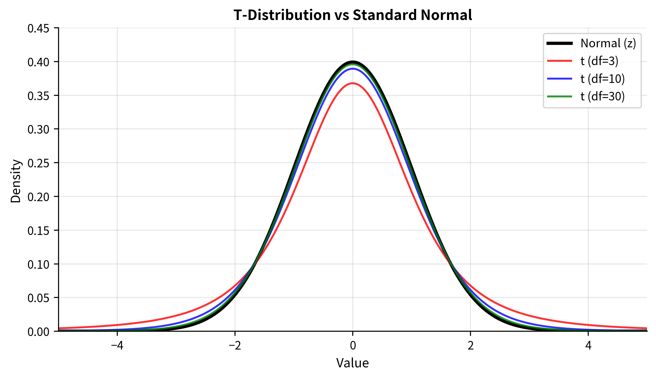
The t-distribution has several key properties:
- Bell-shaped and symmetric: Like the normal distribution, centered at zero under the null hypothesis
- Heavier tails: More probability in the extreme values than the normal distribution
- Parameterized by degrees of freedom: The shape depends on df, with smaller df meaning heavier tails
- Converges to normal: As , the t-distribution approaches the standard normal
The heavier tails are the crucial difference. They reflect the uncertainty added by estimating variance: with small samples, can deviate substantially from , so extreme t-values become more probable. The t-distribution accounts for this by requiring larger critical values to reject the null hypothesis.
Why Heavier Tails Make Sense
Consider what happens when happens to underestimate :
- The denominator is too small
- The t-statistic is inflated
- We might incorrectly reject
When overestimates :
- The denominator is too large
- The t-statistic is deflated
- We might miss a real effect
These errors don't favor either direction on average, but they add variability. The t-distribution captures exactly this additional spread. With only 5 observations (df = 4), the sample standard deviation is quite unreliable, so the t-distribution has very heavy tails. With 100 observations (df = 99), is a much more reliable estimate of , and the t-distribution is nearly identical to the normal.
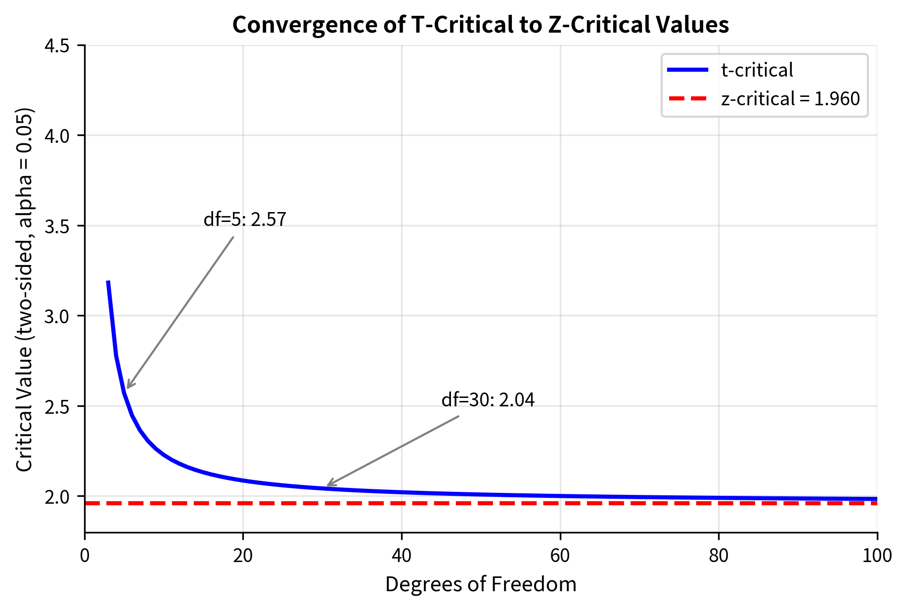
Critical Values: The Practical Impact
The heavier tails translate directly into larger critical values. For a two-sided test at :
| Degrees of Freedom | t-critical | z-critical |
|---|---|---|
| 5 | 2.571 | 1.960 |
| 10 | 2.228 | 1.960 |
| 20 | 2.086 | 1.960 |
| 30 | 2.042 | 1.960 |
| 100 | 1.984 | 1.960 |
| 1.960 | 1.960 |
With df = 5, you need a t-statistic 31% larger than the z-critical value to reject . This penalty appropriately reflects the unreliability of variance estimates from small samples. By df = 30, the difference is only about 4%, which is why older textbooks sometimes said "use z for n > 30." Modern practice uses the t-distribution regardless, as computational tools make it trivially easy.
The One-Sample T-Test
The one-sample t-test compares a sample mean to a hypothesized population value when the population variance is unknown. This is the simplest and most direct application of the t-distribution.
The Complete Procedure
Hypotheses:
- (population mean equals the hypothesized value)
- (two-sided), or / (one-sided)
where:
- = sample mean
- = hypothesized population mean
- = sample standard deviation (with Bessel's correction: divide by )
- = sample size
- = standard error of the mean
Distribution under : (t-distribution with degrees of freedom)
P-value calculation:
- Two-sided: where
- One-sided (greater):
- One-sided (less):
Decision rule: Reject if , or equivalently, if for two-sided tests.
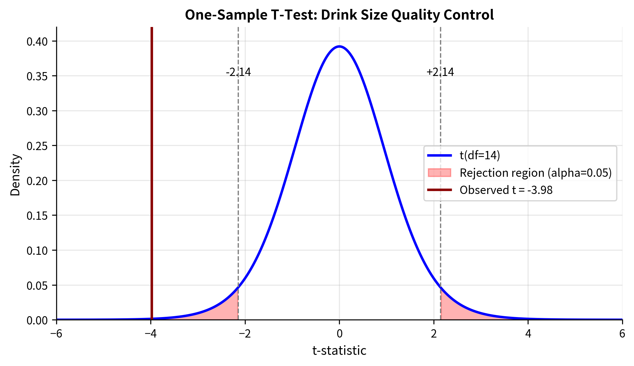
Worked Example: Quality Control
A coffee shop claims their large drinks contain 16 ounces. A quality inspector measures 15 randomly selected drinks to verify this claim.
Let's walk through the calculation step by step:
Step 1: Sample Statistics
Step 2: Standard Error
Step 3: T-Statistic
Step 4: P-Value
With df = 14, we find the probability of observing under :
The Two-Sample T-Test
The two-sample t-test compares means from two independent groups. This is perhaps the most common application: comparing treatment vs. control, method A vs. method B, or any two distinct populations.
A crucial question arises: do the two groups have equal variance? The answer determines which variant of the t-test you should use.
Why Variance Equality Matters
When comparing two means, we need to estimate the standard error of the difference . If both groups share the same variance , we can pool their data to get a more precise estimate. But if variances differ, pooling gives incorrect results, biasing our inference.
This leads to two variants:
- Pooled (Student's) t-test: Assumes equal variances, pools data for efficiency
- Welch's t-test: Makes no variance assumption, handles unequal variances correctly
Pooled Two-Sample T-Test
When we assume , we can estimate this common variance using data from both groups.
Pooled variance estimate:
This is a weighted average of the two sample variances, with weights proportional to their degrees of freedom. Larger samples contribute more to the pooled estimate because they provide more reliable information.
Standard error of the difference:
The term accounts for the fact that uncertainty in the difference comes from uncertainty in both means.
Degrees of freedom:
Each group contributes degrees of freedom for variance estimation, and we combine them.
Welch's T-Test (Recommended Default)
When variances may differ, we cannot pool them. Instead, we estimate standard errors separately and combine them using a different formula.
Standard error of the difference:
This follows from the variance of a difference: for independent samples.
Test statistic:
Degrees of freedom (Welch-Satterthwaite approximation):
This complex formula estimates the effective degrees of freedom when variances are unequal. The result is typically non-integer, which modern software handles through interpolation.
Why Welch's is the recommended default:
- When variances are equal, Welch's test loses only slightly in power compared to the pooled test
- When variances are unequal, the pooled test can give seriously incorrect results
- The asymmetric risk/reward favors Welch's as the default choice
Worked Example: Comparing Teaching Methods
A researcher compares test scores from two teaching methods: Method A (traditional lectures) and Method B (active learning).

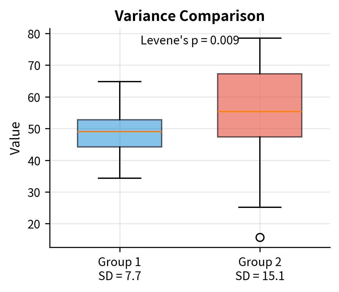
Checking the Equal Variance Assumption
Before choosing between pooled and Welch's tests, you might want to check whether variances are equal. Two common approaches:
1. Visual inspection: Compare the spread in boxplots or calculate the ratio of sample variances. A ratio greater than 2 suggests meaningful inequality.
2. Levene's test: A formal hypothesis test for equality of variances. Unlike older alternatives (Bartlett's test), Levene's test is robust to non-normality.
Many statisticians now recommend always using Welch's t-test as the default, regardless of whether variances appear equal. The reasoning:
- When variances are truly equal, Welch's test loses very little power compared to the pooled test
- When variances are unequal, the pooled test can produce seriously misleading results
- Pre-testing for equal variances adds complexity and has its own issues (low power with small samples, unnecessary when samples are large)
This "Welch by default" approach is increasingly adopted in statistical software and practice.
The Paired T-Test
The paired t-test is used when observations come in matched pairs, where each pair shares some characteristic that makes them non-independent. Common scenarios include:
- Before-after measurements: Same subjects measured twice
- Matched case-control studies: Cases matched to controls on key characteristics
- Twin studies: Comparing outcomes between twins
- Left-right comparisons: Same subject, different sides
Why Pairing Matters
Consider testing whether a training program improves performance. You could:
- Independent design: Randomly assign people to training or control groups, compare group means
- Paired design: Measure each person before and after training, analyze the changes
The paired design is often more powerful because it eliminates between-subject variability. People differ enormously in baseline ability, but by looking at changes within each person, we focus only on the training effect.
The Mathematics
The paired t-test is simply a one-sample t-test on the differences:
where:
- = mean of the paired differences
- = standard deviation of the differences
- = number of pairs
Null hypothesis: (no average change)
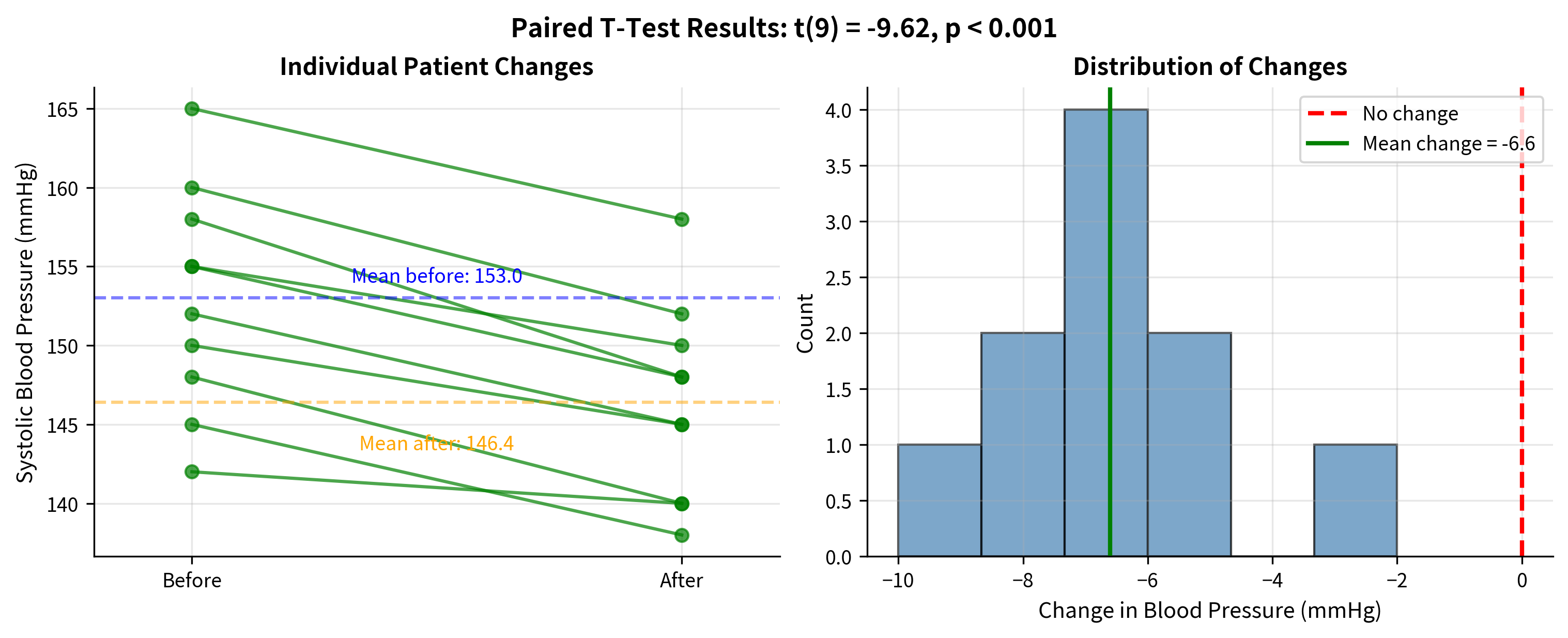
Worked Example: Blood Pressure Medication
A study tests whether a new medication reduces blood pressure. Ten patients have their systolic blood pressure measured before starting medication and again after 4 weeks of treatment.
Why Not Use an Independent T-Test?
You might wonder: what if we ignored the pairing and used an independent two-sample t-test? Let's compare:
The paired test detects the effect with much higher confidence because it accounts for the correlation between before and after measurements within each subject.
Assumptions and Robustness
All t-tests rely on assumptions. Understanding these assumptions, how to check them, and how robust the tests are to violations, is essential for proper application.
Core Assumptions
1. Independence
- One-sample: Observations must be independent of each other
- Two-sample (independent): Observations between groups must be independent; observations within groups must be independent
- Paired: The pairs must be independent of each other (though observations within a pair are dependent by design)
Independence is often the most critical and hardest to verify assumption. It depends on study design rather than data characteristics.
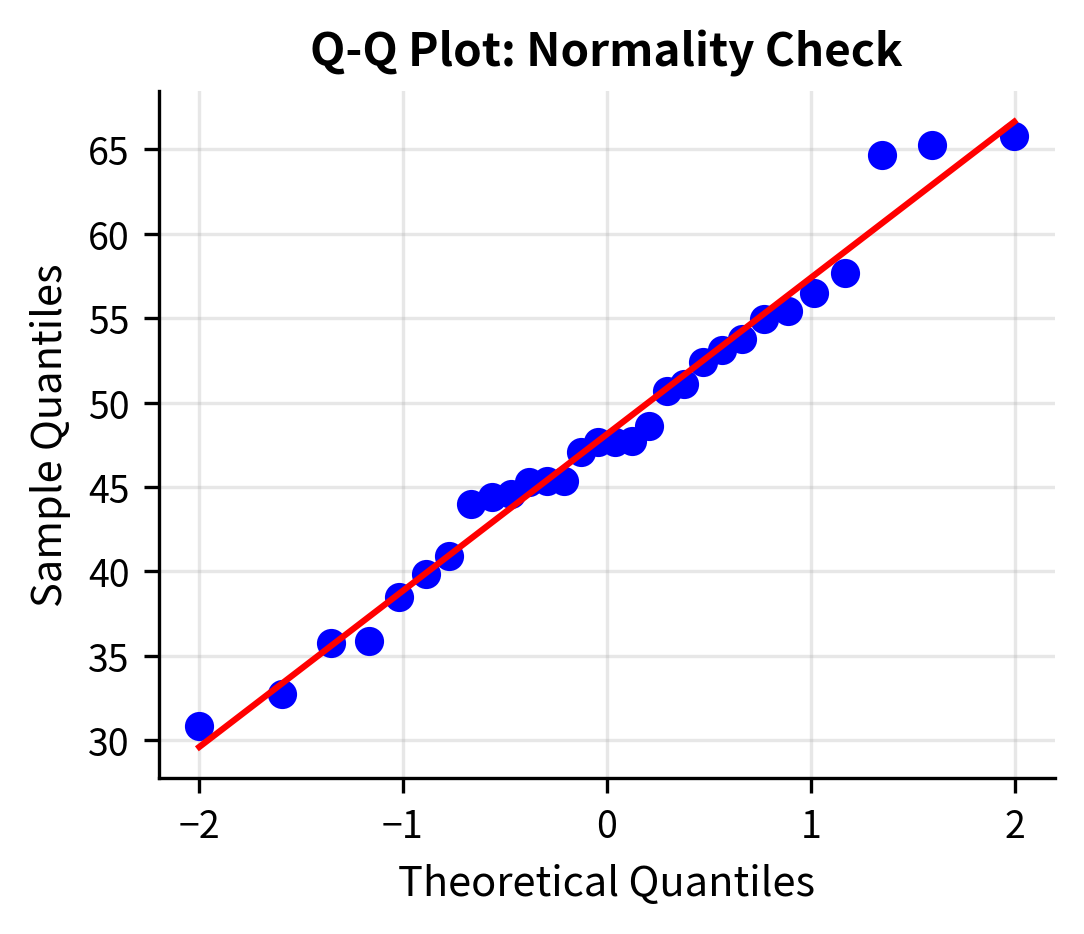
2. Normality
The sampling distribution of the mean should be approximately normal. This is satisfied when:
- The population is normally distributed, OR
- The sample size is large enough for the Central Limit Theorem to apply
Robustness: The t-test is fairly robust to non-normality, especially for:
- Two-sided tests
- Larger sample sizes (n > 30 per group)
- Symmetric distributions
It is less robust for:
- Small samples from highly skewed distributions
- One-sided tests
- Comparing variances or making precise probability statements
3. Homogeneity of Variance (pooled t-test only)
The pooled two-sample t-test assumes equal population variances. Violations affect:
- Type I error rate (can be inflated or deflated)
- The bias is worse with unequal sample sizes
Solution: Use Welch's t-test, which doesn't assume equal variances.
Checking Assumptions
Choosing the Right T-Test: Decision Framework
Selecting the appropriate t-test depends on your research design and data characteristics:
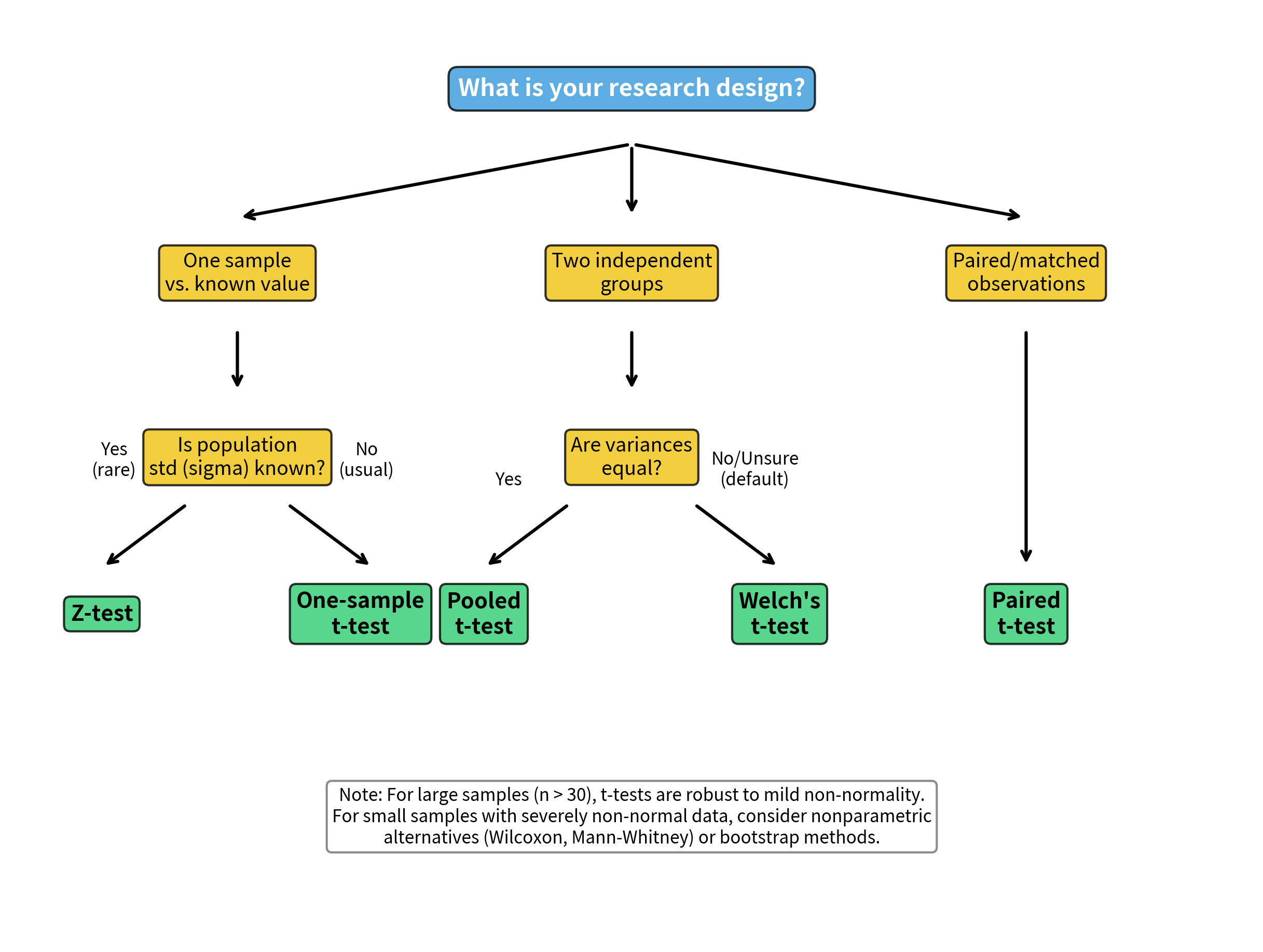
Quick Reference:
| Scenario | Test | scipy.stats function |
|---|---|---|
| One sample vs. hypothesized value | One-sample t-test | ttest_1samp(data, mu_0) |
| Two independent groups (default) | Welch's t-test | ttest_ind(a, b, equal_var=False) |
| Two independent groups (equal variance confirmed) | Pooled t-test | ttest_ind(a, b, equal_var=True) |
| Matched pairs / before-after | Paired t-test | ttest_rel(after, before) |
Summary
The t-test is the fundamental tool for comparing means when population variance is unknown, which is nearly always. Key takeaways:
The t-distribution:
- Accounts for uncertainty from estimating variance
- Has heavier tails than the normal distribution
- Converges to normal as degrees of freedom increase
- Requires larger critical values for small samples
One-sample t-test:
- Compares sample mean to hypothesized value
- Test statistic:
- Degrees of freedom:
Two-sample t-test:
- Compares means from two independent groups
- Pooled variant assumes equal variances
- Welch's variant (recommended default) handles unequal variances
- Degrees of freedom differ between variants
Paired t-test:
- For matched pairs or repeated measures
- Analyzes within-pair differences
- Often more powerful than independent tests by eliminating between-subject variability
Assumptions:
- Independence (critical, design-based)
- Normality (robust for large samples)
- Equal variances (pooled test only; avoid by using Welch's)
When in doubt: Use Welch's t-test for two-sample comparisons. You sacrifice minimal power when variances are equal but gain robustness when they differ.
What's Next
This chapter covered t-tests for comparing one or two means. But what if you want to compare variances rather than means? Or compare more than two groups? The next chapters extend these ideas:
-
The F-Test introduces the F-distribution for comparing variances. This is important both as a standalone test (are two groups equally variable?) and as foundation for ANOVA.
-
ANOVA extends the t-test to compare three or more groups simultaneously, avoiding the multiple comparison problems that arise from running many t-tests.
-
Error types, statistical power, effect sizes, and multiple comparison corrections are all essential for interpreting and designing studies that use t-tests and related methods.
The t-test you've learned here is the building block for all these extensions. Master it, and the more advanced methods will follow naturally.
Quiz
Ready to test your understanding? Take this quick quiz to reinforce what you've learned about the t-test.

Comments