

Complete guide to z-tests including one-sample, two-sample, and proportion tests. Learn when to use z-tests, how to calculate test statistics, and interpret results when population variance is known.

This article is part of the free-to-read Machine Learning from Scratch
Choose your expertise level to adjust how many terms are explained. Beginners see more tooltips, experts see fewer to maintain reading flow. Hover over underlined terms for instant definitions.
The Z-Test
You've learned what p-values mean. You understand how to set up null and alternative hypotheses. You know what assumptions matter. Now it's time to put all of that knowledge into practice with your first complete hypothesis test.
The z-test is the natural starting point because it's the simplest parametric test. When you know the population standard deviation, the z-test gives you exact inference based on the familiar normal distribution. No approximations, no complex formulas, just a straightforward application of everything you've learned so far.
But here's the thing: knowing the population standard deviation is rare in practice. So why learn the z-test at all? Two reasons. First, it's the foundation for understanding more complex tests like the t-test (next chapter). Second, z-tests are the standard approach for testing proportions, which is one of the most common hypothesis testing scenarios in data science, from A/B testing to clinical trials to quality control.
When Should You Use a Z-Test?
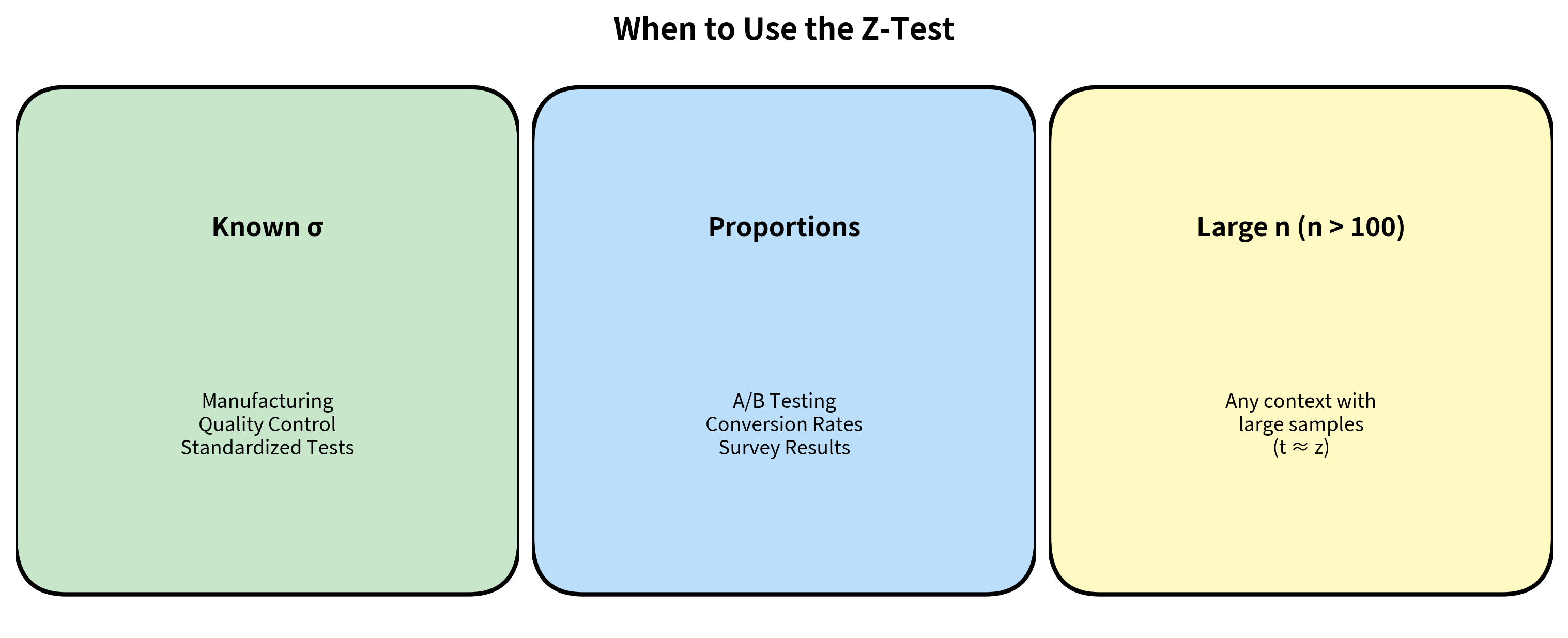
The z-test is appropriate in three scenarios:
Scenario 1: Known Population Standard Deviation
This is rare but does occur:
- Calibrated measurement systems: Manufacturing processes often have extensively characterized measurement instruments where σ is known from calibration studies
- Standardized tests: IQ tests, for example, are designed to have σ = 15 in the general population
- Quality control: When historical data from millions of measurements establishes σ reliably
Scenario 2: Testing Proportions
This is the most common real-world use of z-tests. When testing hypotheses about population proportions, the variance is determined by the proportion itself (). You don't need to estimate it separately, so the z-test is appropriate.
Scenario 3: Very Large Samples
When sample sizes exceed 100 or so, the t-distribution converges to the normal distribution. In these cases, z-tests and t-tests give essentially identical results. However, using the t-test is never wrong even with large samples, so there's no real advantage to using z here.
The Z-Test Formula: A Deep Dive
The Core Formula
The z-test statistic is:
This formula looks simple, but each component has deep meaning. Let's understand why this particular combination of quantities gives us exactly what we need for hypothesis testing.
Step 1: The Numerator Measures the Discrepancy
This is the difference between what you observed (sample mean ) and what the null hypothesis claims (population mean ).
Example: If the null hypothesis claims the population mean is 100 and you observe a sample mean of 95, the numerator is .
But here's the problem: a difference of 5 could be huge or trivial depending on context. If you're measuring heights in millimeters, 5 mm is negligible. If you're measuring earthquake magnitudes, 5 points is catastrophic. We need to standardize.
Step 2: The Denominator Provides Context
This is the standard error, and it answers: "How much do sample means typically vary from sample to sample?"
The standard error depends on two factors:
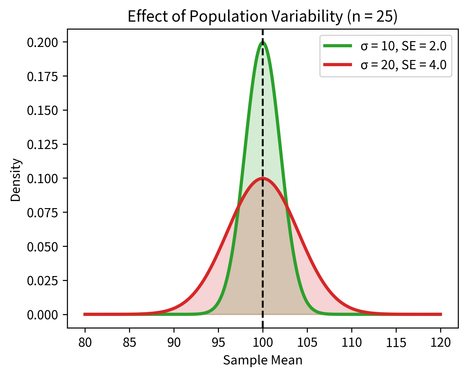
Factor 1: Population variability (σ)
More variable populations produce more variable sample means. If individual observations vary a lot, the averages of groups of observations will also vary.
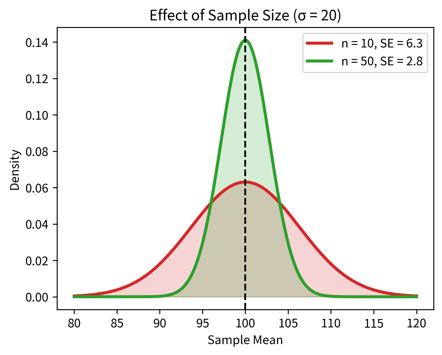
Factor 2: Sample size (n)
Larger samples produce more stable estimates. The in the denominator reflects a fundamental principle: averaging reduces noise. When you average n independent observations, random fluctuations tend to cancel out.
Step 3: The Ratio Gives Standardized Evidence
When you divide the observed discrepancy by the standard error:
You get a standardized score that tells you: "How many standard errors away from the null hypothesis is my observation?"
- means your sample mean is 1 standard error away from
- means your sample mean is 2 standard errors away
- means your sample mean is 1.5 standard errors below
The beauty of standardization is that it puts all tests on the same scale. Whether you're measuring heights, weights, temperatures, or dollars, a z-score of 2 always has the same interpretation: your observation is 2 standard errors from what the null predicts.
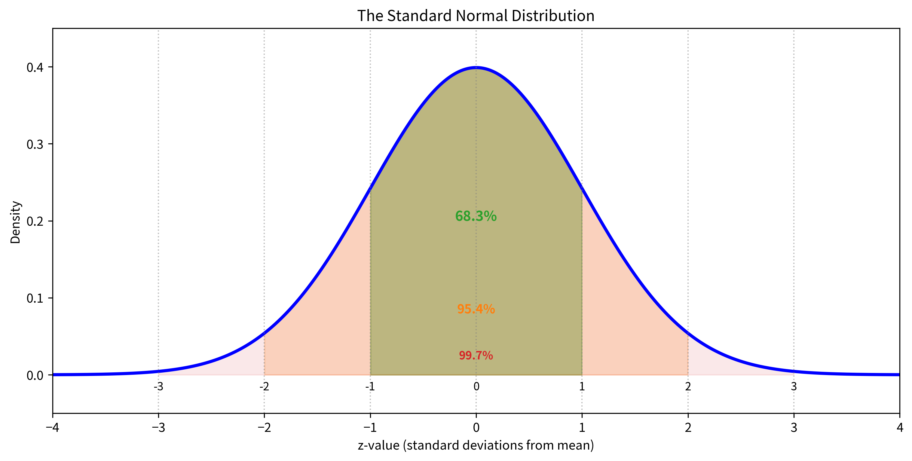
Why the Standard Normal Distribution?
Under the null hypothesis , if either:
- The population is normally distributed, OR
- The sample size is large enough for the Central Limit Theorem to apply
Then the z-statistic follows a standard normal distribution .
This is the key insight that makes z-tests work. We know everything about the standard normal distribution. We can calculate exact probabilities for any z-value. So once we compute z, we can immediately determine how surprising our result is under the null hypothesis.
Computing P-Values from Z-Statistics
Once you have a z-statistic, you need to convert it to a p-value. The process depends on whether you're doing a one-sided or two-sided test.
Two-Sided Test
For a two-sided test (testing whether the mean differs from in either direction):
where is the standard normal CDF. We double the probability because we're interested in extreme values in both tails.
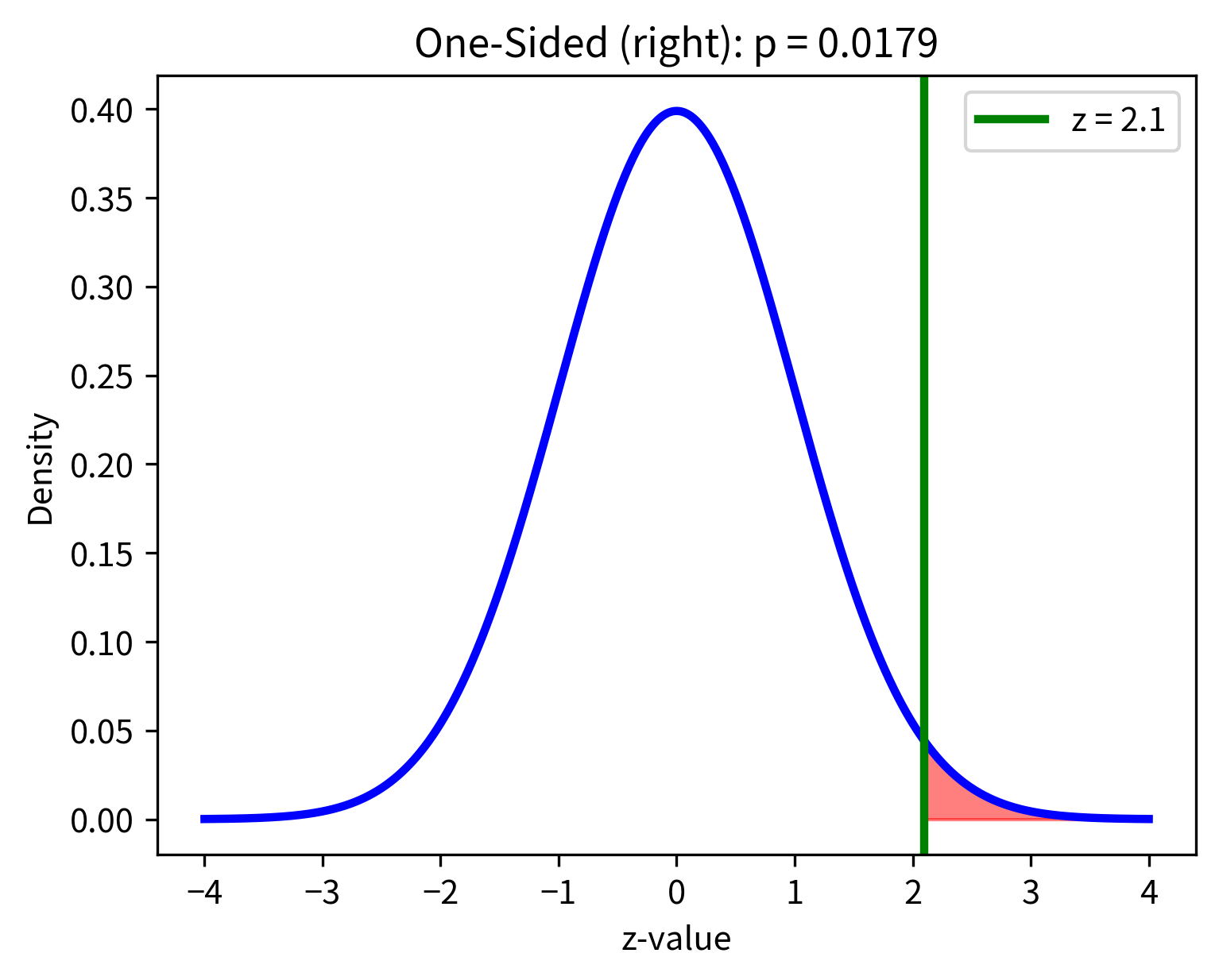
One-Sided Tests
For a right-tailed test (testing whether the mean is greater than ):
For a left-tailed test (testing whether the mean is less than ):

One-Sample Z-Test: Complete Worked Example
Let's work through a complete example with every calculation shown explicitly.
The Problem
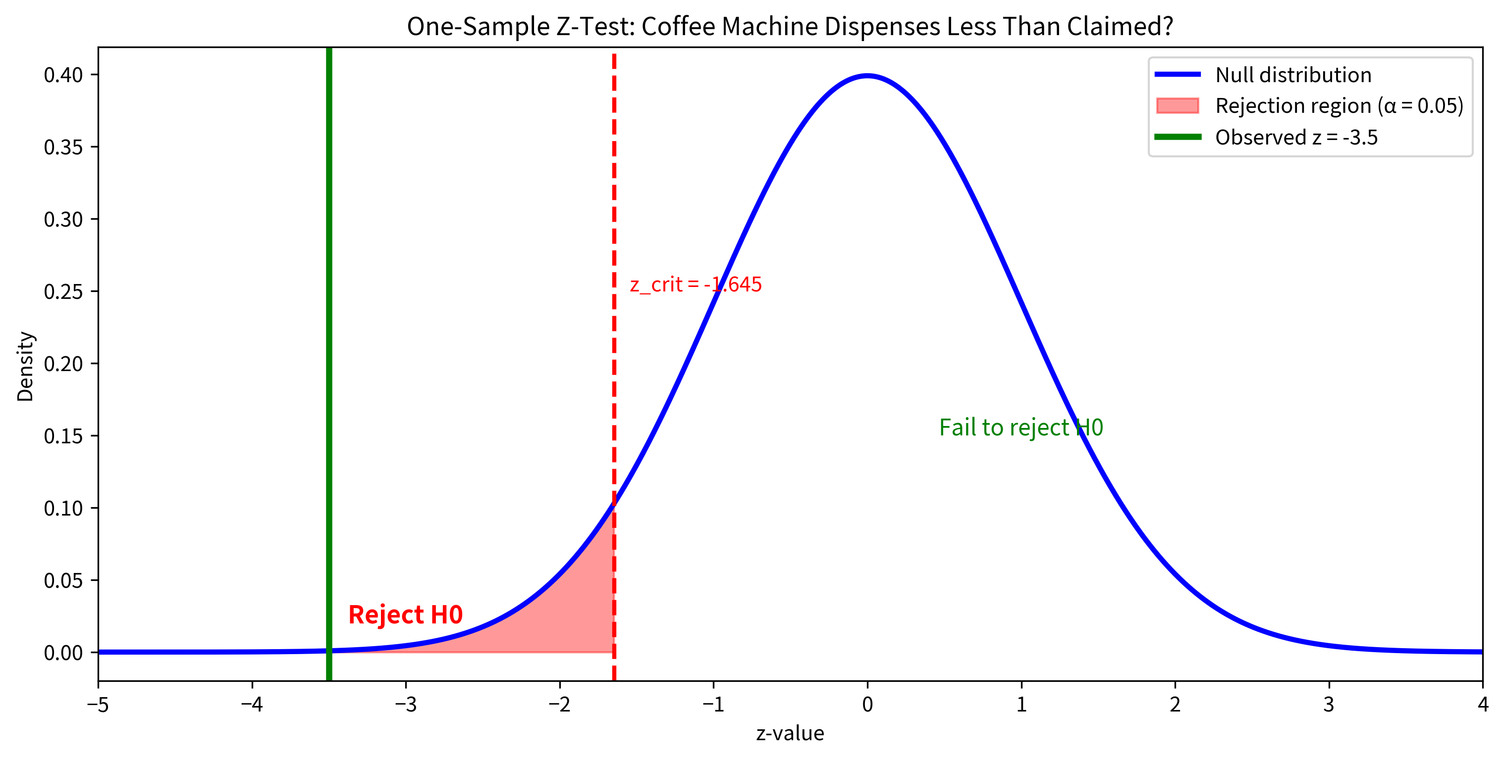
A coffee machine manufacturer claims their machines dispense exactly 200 mL per cup, with a known standard deviation of 5 mL (established through extensive quality testing). A consumer group tests 49 cups from a randomly selected machine and finds a mean of 197.5 mL. Is there evidence that this machine dispenses less than the claimed amount?
Step 1: State the Hypotheses
Since we're specifically asking whether the machine dispenses less than claimed, this is a one-sided test:
- (The machine dispenses the claimed amount)
- (The machine dispenses less than claimed)
Step 2: Identify the Known Values
- Sample mean: mL
- Hypothesized mean: mL
- Population standard deviation: mL
- Sample size:
- Significance level:
Step 3: Calculate the Standard Error
This tells us that sample means of 49 cups typically vary by about 0.714 mL from the true population mean.
Step 4: Calculate the Z-Statistic
The sample mean is 3.50 standard errors below the hypothesized value. This is quite extreme!
Step 5: Calculate the P-Value
For a left-tailed test:
Step 6: Make a Decision
Since , we reject the null hypothesis. There is strong evidence that the machine dispenses less than 200 mL per cup.
Confidence Interval Interpretation
We can also construct a 95% confidence interval for the true mean:
Two-Sample Z-Test
When comparing means from two independent populations with known variances, we use the two-sample z-test.
The Formula
Where:
- : Sample means from groups 1 and 2
- : Hypothesized difference (usually 0 for testing equality)
- : Known population standard deviations
- : Sample sizes
Why Do Variances Add?
When you subtract two independent random variables, their variances add:
This might seem counterintuitive (why add when we're subtracting?), but it makes sense when you think about it: the difference between two uncertain quantities is more uncertain than either quantity alone. Uncertainty compounds.
Example: Comparing Two Production Lines
A factory has two production lines making the same component. Historical quality data shows Line A has units and Line B has units. A sample of 40 items from Line A has mean 50.2, and a sample of 50 items from Line B has mean 48.7. Do the lines produce different mean outputs?
The p-value of about 0.008 provides strong evidence that the two lines have different mean outputs. The 95% CI for the difference [0.39, 2.61] doesn't include 0, consistent with our rejection of the null hypothesis.
Z-Test for Proportions
The z-test for proportions is the most common real-world application of z-tests. It's used extensively in A/B testing, survey analysis, clinical trials, and quality control.
Why Z-Tests Work for Proportions
For a binomial proportion, the variance is determined by the proportion itself:
Under the null hypothesis , we use to calculate the standard error:
The test statistic is:
where is the sample proportion (x successes out of n trials).
When Is the Normal Approximation Valid?
The z-test for proportions uses the normal approximation to the binomial. This works well when:
- (expected successes)
- (expected failures)
For smaller samples or proportions near 0 or 1, use exact binomial tests instead.
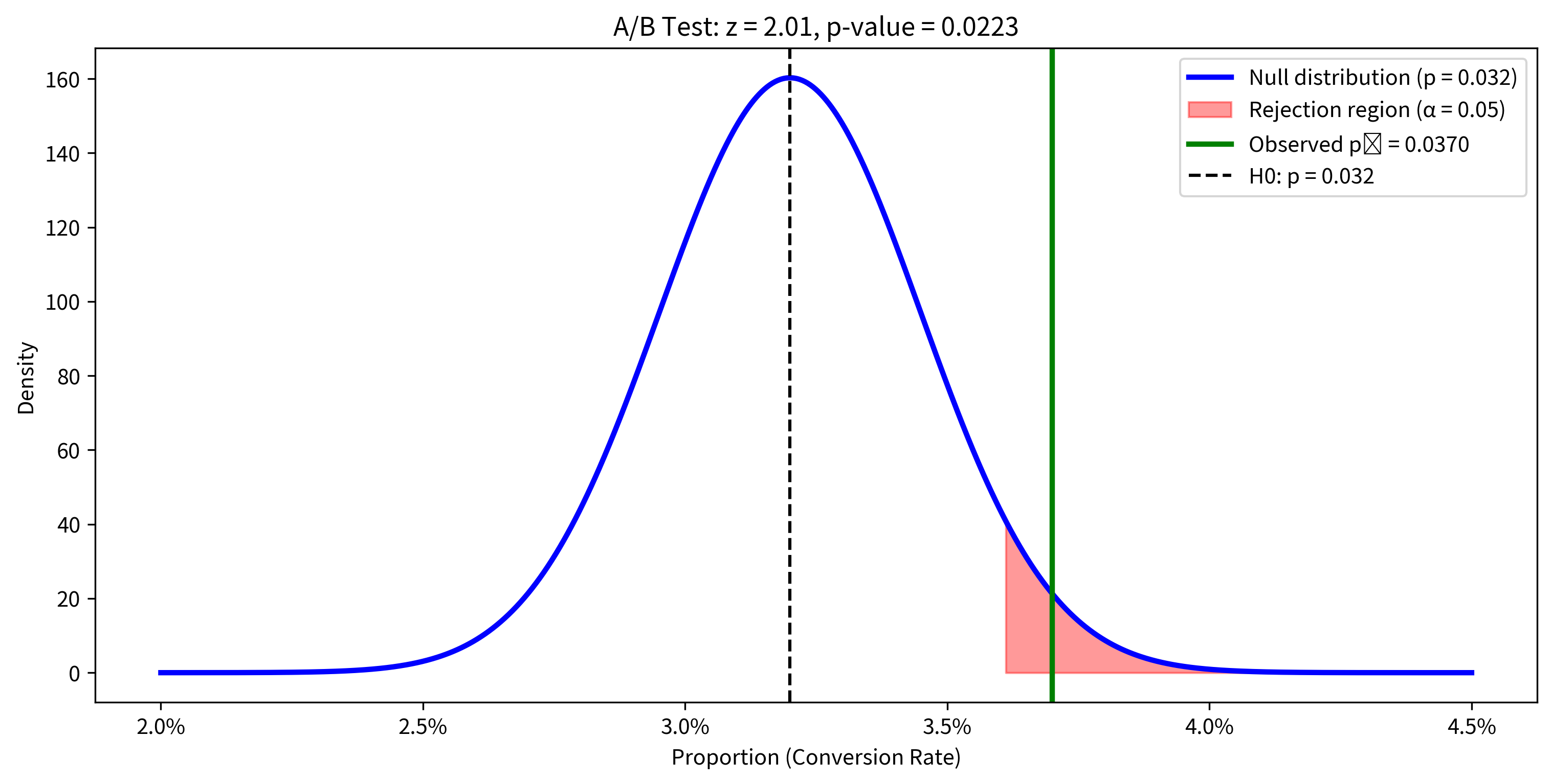
Example: A/B Testing
An e-commerce company wants to test whether a new checkout design improves their conversion rate. Their current conversion rate is 3.2%. After showing the new design to 5000 visitors, 185 converted. Is there evidence of improvement?
The p-value of about 0.034 is less than 0.05, so we have evidence that the new design improves conversion rates. The improvement from 3.2% to 3.7% represents a 15.6% relative increase.
Two-Sample Proportion Test
When comparing proportions from two groups (e.g., control vs treatment), use:
Where is the pooled proportion under the null hypothesis that .
Relationship to the T-Test
The z-test and t-test are closely related. The key differences:
| Aspect | Z-Test | T-Test |
|---|---|---|
| Population σ | Known | Unknown (estimated from sample) |
| Test statistic distribution | Standard normal | t-distribution |
| Tail heaviness | Lighter tails | Heavier tails (especially for small n) |
| Critical values | Fixed (e.g., ±1.96 for 95%) | Depend on degrees of freedom |
As sample size increases, the t-distribution converges to the normal distribution. For n > 100, the difference is negligible.
Rule of thumb: If you're unsure whether to use a z-test or t-test, use the t-test. It's valid in all cases where the z-test is valid, plus it handles the much more common case where σ is unknown.
Summary
This chapter covered the z-test comprehensively:
When to Use Z-Tests
- Known population standard deviation (rare for means)
- Testing proportions (most common application)
- Very large samples where t ≈ z
The Core Mathematics
- Test statistic:
- Under , z follows a standard normal distribution
- The standard error quantifies how much sample means vary
Test Procedures
- One-sample z-test: Test whether a mean differs from a specific value
- Two-sample z-test: Test whether two means differ from each other
- Proportion z-test: Test hypotheses about population proportions
- Two-proportion z-test: Compare proportions between groups (A/B testing)
Key Points
- Always verify normal approximation conditions for proportion tests
- Confidence intervals provide the same information as hypothesis tests
- The z-test is foundational for understanding more complex tests
What's Next
In the next chapter, The T-Test, we tackle the far more common situation: testing hypotheses when the population standard deviation is unknown. The t-test uses the sample standard deviation instead, which introduces additional uncertainty accounted for by the t-distribution's heavier tails.
You'll learn about one-sample t-tests, independent two-sample t-tests (including Welch's robust version), and paired t-tests for dependent samples. The conceptual framework is identical to what you've learned here; only the distribution changes.
After t-tests, subsequent chapters cover F-tests for comparing variances, ANOVA for comparing multiple groups, and advanced topics including power analysis, effect sizes, and multiple comparison corrections.
Quiz
Ready to test your understanding? Take this quick quiz to reinforce what you've learned about the z-test.

Comments