

One-way ANOVA, post-hoc tests, assumptions, and when to use ANOVA. Learn how to compare means across three or more groups while controlling Type I error rates.

This article is part of the free-to-read Machine Learning from Scratch
Choose your expertise level to adjust how many terms are explained. Beginners see more tooltips, experts see fewer to maintain reading flow. Hover over underlined terms for instant definitions.
ANOVA (Analysis of Variance)
Imagine you're running a clinical trial comparing four different medications for lowering blood pressure. You've recruited patients, randomly assigned them to treatment groups, and measured their outcomes. Now you need to determine: do any of these medications work differently from the others?
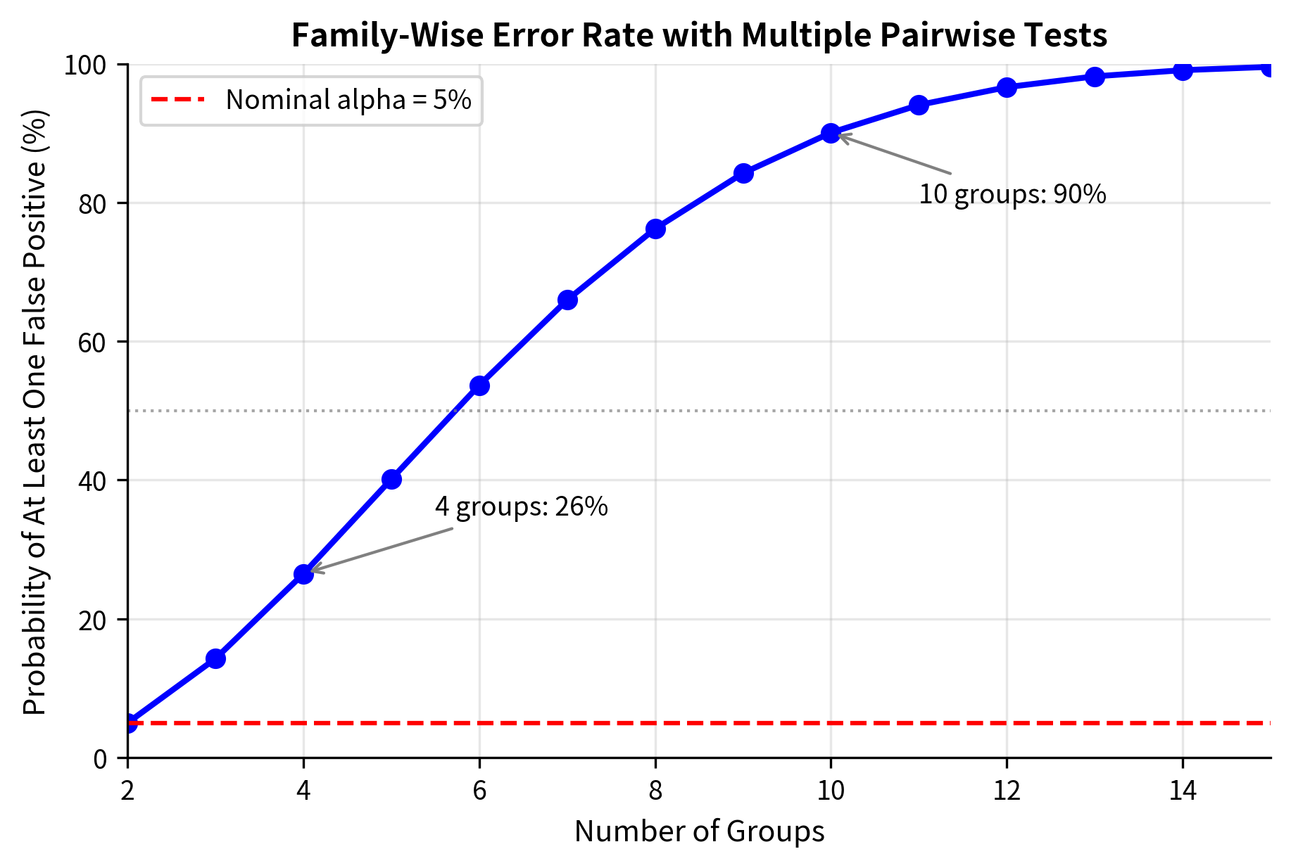
Your first instinct might be to run t-tests comparing each pair of medications: Drug A vs B, A vs C, A vs D, B vs C, B vs D, and C vs D. That's six separate tests. But here's the problem: even if all four drugs are equally effective (no real differences), you'd falsely conclude that at least one pair differs about 26% of the time, not the 5% you expect from a single test at . With more groups, this gets worse. Ten groups would require 45 pairwise comparisons, with a false positive rate exceeding 90%.
This is the multiple comparisons problem, and it's why Analysis of Variance (ANOVA) exists. ANOVA tests whether any group means differ using a single test that maintains your chosen Type I error rate. Developed by Ronald Fisher in the 1920s for agricultural experiments, ANOVA has become one of the most widely used statistical techniques in science, medicine, psychology, and industry.
This chapter builds directly on the F-distribution and F-tests you learned previously. ANOVA uses the same logic: partition total variation into components, then test whether the ratio of variance estimates is larger than expected by chance. By the end of this chapter, you'll understand not just how to perform ANOVA, but why it works and when to use it.
The Multiple Comparisons Problem
Before diving into ANOVA, let's understand exactly why multiple t-tests fail.
When you conduct a single hypothesis test at , you accept a 5% chance of a Type I error (false positive) when the null is true. But with multiple tests, each test adds another opportunity for error.
The probability of at least one false positive across independent tests is:
For :
| Number of Groups | Pairwise Comparisons | P(At least one Type I error) |
|---|---|---|
| 3 | 3 | 14.3% |
| 4 | 6 | 26.5% |
| 5 | 10 | 40.1% |
| 10 | 45 | 90.1% |
This explosion of false positives makes multiple t-tests unreliable. ANOVA solves this by asking a single question: "Do any of the group means differ?" rather than asking many questions about specific pairs.
The Logic of ANOVA: Comparing Variances to Test Means
ANOVA's name, "Analysis of Variance," seems paradoxical. If we want to compare means, why analyze variances? The genius of ANOVA lies in recognizing that differences among means manifest as a specific pattern of variance.
The Core Insight
Consider three groups with potentially different population means , , and . When we collect samples from these groups, we observe two types of variation:
1. Within-group variation: How much individuals vary around their own group mean. This reflects natural variability in the data, measurement error, and individual differences. Crucially, this variation exists regardless of whether the population means differ.
2. Between-group variation: How much the group means vary around the overall (grand) mean. This reflects sampling variation plus any true differences among population means.
Here's the key insight: if all population means are equal, the between-group variation should be similar to what we'd expect from sampling variation alone. The group means will differ somewhat, but only because of random sampling, not because the populations are truly different.
But if population means differ, the between-group variation will be inflated beyond what sampling alone would produce. The group means will be more spread out than chance would predict.
ANOVA formalizes this by computing the ratio:
- If : Between and within variation are similar; no evidence of mean differences
- If : Between variation is much larger than within; evidence that means differ

The Mathematics of One-Way ANOVA
Let's formalize these ideas mathematically. One-way ANOVA compares means across groups, where "one-way" means there's a single grouping factor.
Notation
- = number of groups
- = sample size of group (for )
- = total sample size
- = observation in group
- = mean of group
- = grand mean (overall mean)
The ANOVA Decomposition
The total variation in the data can be decomposed into two components:
Let's understand each component:
Total Sum of Squares (): Measures total variation in the data. Each observation's squared deviation from the grand mean, summed across all observations. This is the same quantity we'd use to compute variance of the entire dataset.
Between-Group Sum of Squares (): Measures variation of group means around the grand mean. Each group mean's squared deviation from the grand mean, weighted by sample size. Larger groups contribute more because their means are more reliable.
Within-Group Sum of Squares (): Measures variation within each group. Each observation's squared deviation from its own group mean, summed across all groups. This represents the "noise" or baseline variability.
From Sums of Squares to Mean Squares
Sums of squares grow with sample size, so we convert them to mean squares (variance estimates) by dividing by degrees of freedom:
Why these degrees of freedom?
- Between-groups (): We have group means, but they must average to the grand mean (one constraint), leaving independent pieces of information.
- Within-groups (): We have observations, but we estimate group means (one per group), losing degrees of freedom.
The F-Statistic
The F-statistic is the ratio of mean squares:
Under the null hypothesis that all population means are equal (), this F-statistic follows an F-distribution with and degrees of freedom.
Intuition:
- estimates (the common variance within groups) regardless of whether the null is true
- estimates only if the null is true; if means differ, it estimates something larger
- If is true, ; if is false,
The Hypotheses
Null hypothesis: (all population means are equal)
Alternative hypothesis: At least one population mean differs from the others
Note that rejecting tells us that some means differ, but not which ones. For that, we need post-hoc tests (discussed later).
Worked Example: Comparing Fertilizers
A agricultural researcher tests three fertilizers to see if they produce different plant growth. She randomly assigns 10 plants to each fertilizer and measures growth (in cm) after 6 weeks.
Let's trace through the calculation step by step:
Step 1: Basic Statistics
Step 2: Sum of Squares Between
Step 3: Sum of Squares Within
Step 4: Mean Squares and F-Statistic
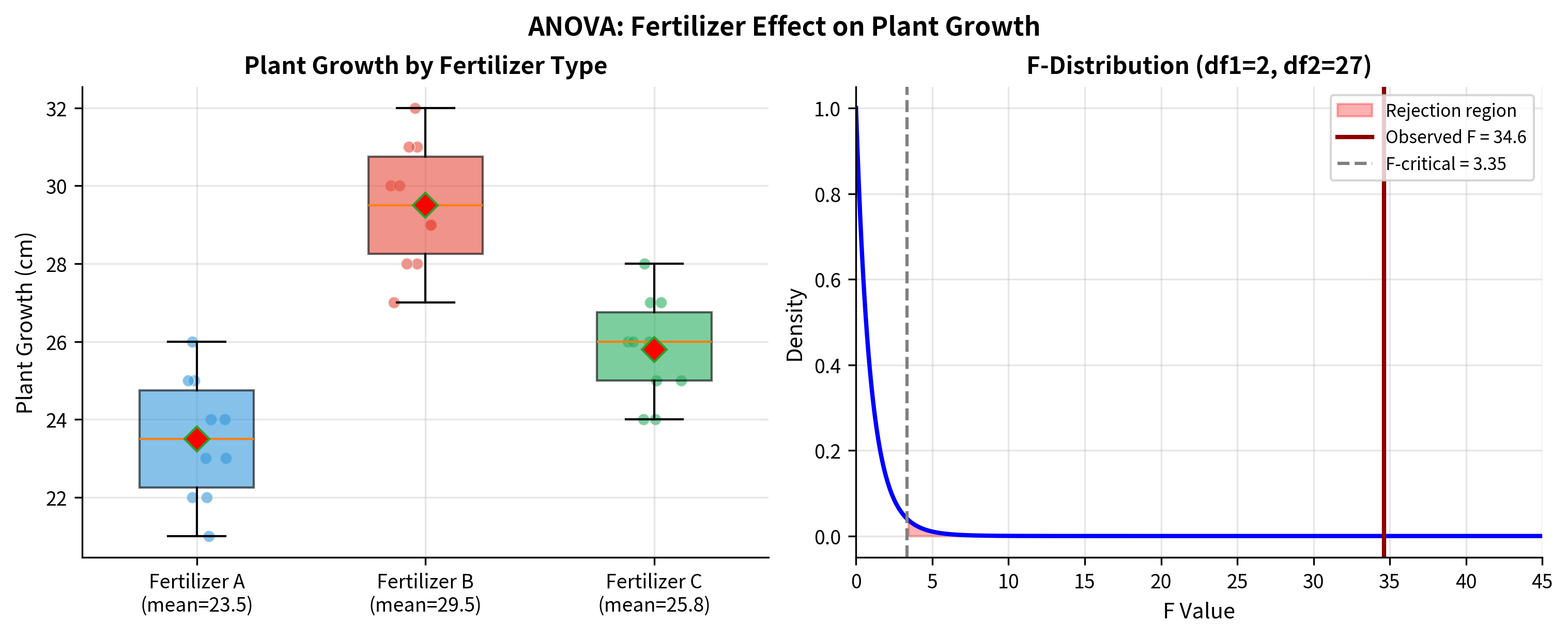
The ANOVA reveals a highly significant difference among fertilizers (, ). The effect size indicates that 72% of the variation in plant growth is explained by fertilizer type, a very large effect.
Post-Hoc Tests: Which Groups Differ?
When ANOVA rejects the null hypothesis, we know at least one group mean differs from the others, but not which specific pairs differ. Post-hoc tests make pairwise comparisons while controlling the family-wise error rate.
The Need for Multiple Comparison Corrections
Without correction, testing all pairwise differences would inflate the Type I error rate, exactly the problem ANOVA was designed to solve. Post-hoc tests apply corrections to maintain the overall error rate at .
Tukey's Honest Significant Difference (HSD)
Tukey's HSD is the most commonly used post-hoc test for ANOVA. It controls the family-wise error rate while comparing all pairs of means.
The test compares the difference between any two group means to a critical value based on the studentized range distribution:
where is the critical value from the studentized range distribution.
Two means are significantly different if .
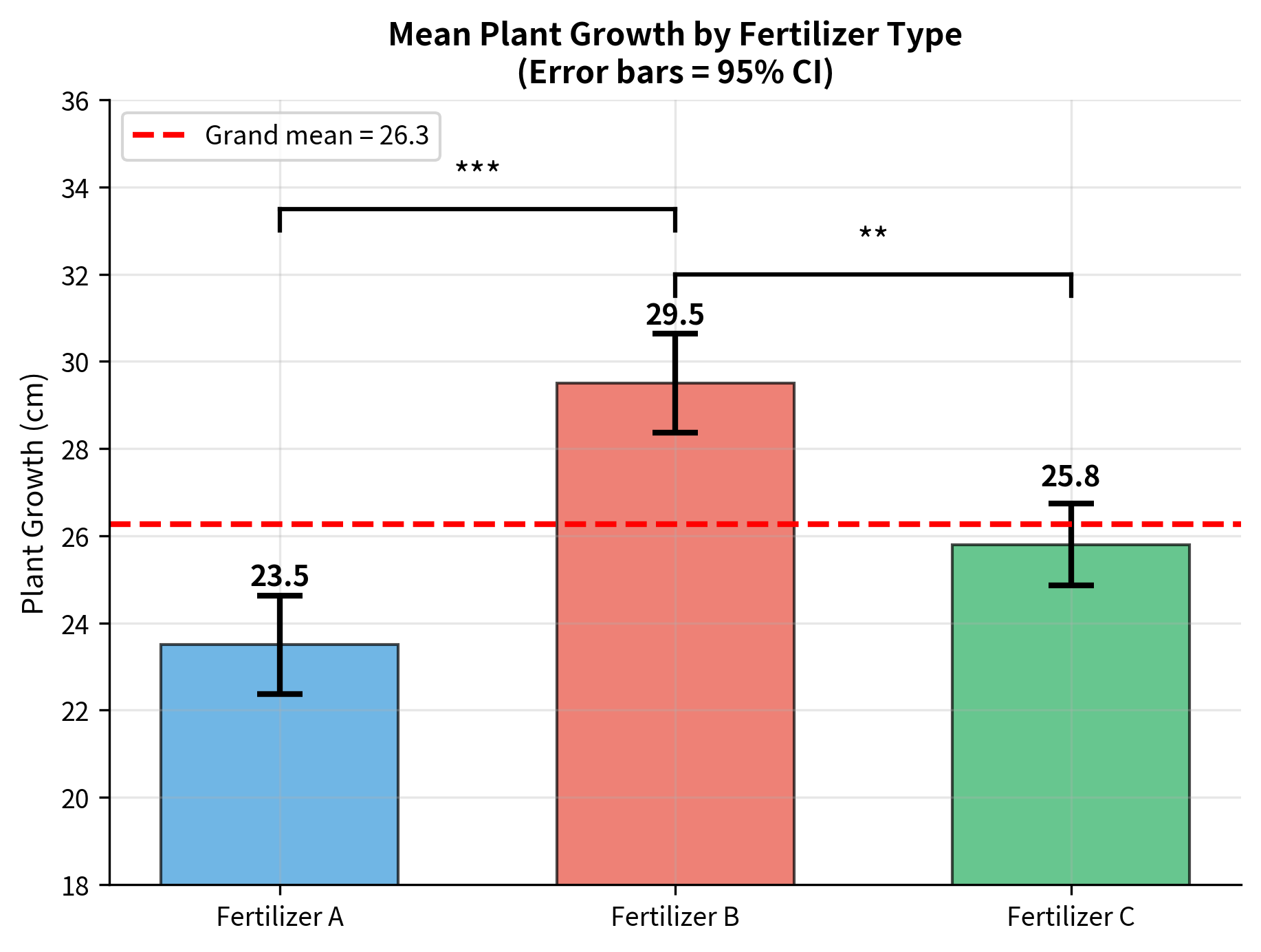
The post-hoc analysis reveals:
- Fertilizer B produces significantly more growth than both A and C
- Fertilizers A and C do not differ significantly from each other
This is consistent with the visual impression from the boxplots: Fertilizer B is clearly the best performer.
Effect Size: Eta-Squared
Statistical significance tells us whether an effect exists, but not how large it is. Effect size measures quantify practical significance.
Eta-Squared ()
The most common effect size for ANOVA is eta-squared:
This represents the proportion of total variance explained by group membership. It ranges from 0 to 1:
| Interpretation | |
|---|---|
| 0.01 | Small effect |
| 0.06 | Medium effect |
| 0.14+ | Large effect |
In our fertilizer example, is a very large effect: fertilizer type explains 72% of the variation in plant growth.
Omega-Squared ()
Eta-squared tends to overestimate the population effect size. Omega-squared provides a less biased estimate:
Assumptions of ANOVA
Like the t-test, ANOVA relies on several assumptions. Understanding these helps you interpret results appropriately and choose alternatives when needed.
1. Independence
Observations must be independent both within and between groups. This is primarily a study design issue:
- Random sampling from populations
- Random assignment to treatment groups
- No clustering or repeated measures (for one-way ANOVA)
2. Normality
Data within each group should be approximately normally distributed. ANOVA is moderately robust to violations of normality, especially when:
- Sample sizes are similar across groups
- Sample sizes are reasonably large (n > 15-20 per group)
- Distributions are not extremely skewed
For small samples or severely non-normal data, consider the Kruskal-Wallis test (non-parametric alternative).
3. Homogeneity of Variance (Homoscedasticity)
All groups should have similar variances. This assumption is important because the F-test uses a pooled variance estimate.
Checking: Use Levene's test or visual inspection of group spreads.
When Assumptions Are Violated
| Violation | Alternative |
|---|---|
| Non-normality | Kruskal-Wallis test |
| Unequal variances | Welch's ANOVA |
| Both | Kruskal-Wallis or permutation test |
Visualizing ANOVA Results
Good visualization helps communicate ANOVA findings effectively.
When to Use ANOVA vs. Other Tests
| Scenario | Recommended Test |
|---|---|
| 2 groups, comparing means | t-test |
| 3+ groups, comparing means | One-way ANOVA |
| 3+ groups, non-normal data | Kruskal-Wallis |
| 3+ groups, unequal variances | Welch's ANOVA |
| Multiple factors | Two-way ANOVA, factorial ANOVA |
| Repeated measures | Repeated measures ANOVA |
Summary
Analysis of Variance (ANOVA) is a powerful technique for comparing means across three or more groups while maintaining control over the Type I error rate.
Core concepts:
- ANOVA compares variances to test means: between-group variation vs. within-group variation
- If group means truly differ, between-group variance will be inflated relative to within-group variance
- The F-statistic is the ratio of these variance estimates
The ANOVA decomposition:
The F-statistic:
Key results:
- ANOVA tests the omnibus hypothesis: are all means equal?
- A significant F-test indicates at least one mean differs, but not which ones
- Post-hoc tests (like Tukey's HSD) identify specific pairwise differences
- Effect sizes (, ) quantify the magnitude of group differences
Assumptions:
- Independence of observations
- Normality within groups (moderately robust)
- Equal variances across groups (Levene's test to check)
When assumptions fail:
- Unequal variances: Welch's ANOVA
- Non-normality: Kruskal-Wallis test
What's Next
This chapter covered one-way ANOVA for comparing means across multiple groups. The following chapters extend your understanding of hypothesis testing:
-
Type I and Type II Errors explores the two ways hypothesis tests can fail: false positives and false negatives. Understanding these errors is essential for interpreting ANOVA results and designing studies.
-
Power and Sample Size shows how to plan studies with adequate power to detect meaningful effects, connecting directly to the effect sizes you learned to calculate here.
-
Effect Sizes provides deeper coverage of measuring practical significance, including alternatives to eta-squared and guidelines for interpretation.
-
Multiple Comparisons revisits the family-wise error rate problem in depth, covering correction methods like Bonferroni, Holm, and false discovery rate control.
The ANOVA framework you've learned here extends naturally to more complex designs: two-way ANOVA (two grouping factors), factorial ANOVA (multiple factors with interactions), and repeated measures ANOVA (same subjects measured multiple times). These advanced topics build directly on the variance decomposition logic you now understand.
Quiz
Ready to test your understanding? Take this quick quiz to reinforce what you've learned about ANOVA.

Comments