Type I and Type II Errors: False Positives, False Negatives & Statistical Power

Michael Brenndoerfer

Data, Analytics & AI Machine Learning Machine Learning from Scratch

Understanding false positives, false negatives, statistical power, and the tradeoff between error types. Learn how to balance Type I and Type II errors in study design.

Reading Level

Choose your expertise level to adjust how many terms are explained. Beginners see more tooltips, experts see fewer to maintain reading flow. Hover over underlined terms for instant definitions.

Type I and Type II ErrorsLink Copied

In 1999, British solicitor Sally Clark was convicted of murdering her two infant sons, who had died suddenly in 1996 and 1998. The prosecution's star witness, pediatrician Sir Roy Meadow, testified that the probability of two children in an affluent family dying from Sudden Infant Death Syndrome (SIDS) was 1 in 73 million. This number, obtained by squaring the 1 in 8,543 probability of a single SIDS death, seemed to prove Clark's guilt beyond any reasonable doubt.

But the calculation was catastrophically wrong. It assumed the two deaths were independent events, ignoring known genetic and environmental factors that make SIDS more likely in families who have already experienced it. More importantly, even if the probability were correct, it confused two very different questions: "What is the probability of two SIDS deaths?" versus "Given two infant deaths, what is the probability the mother is a murderer rather than a victim of tragic coincidence?"

Clark spent three years in prison before her conviction was overturned. The court recognized what statisticians call the prosecutor's fallacy: confusing the probability of the evidence given innocence with the probability of innocence given the evidence. Sally Clark's case illustrates the devastating real-world consequences of misunderstanding error rates in hypothesis testing.

Every statistical test involves making a decision under uncertainty, and every decision carries the risk of error. Understanding these errors, their nature, their probabilities, and the tradeoffs between them, is essential for anyone who uses statistics to make decisions.

The Two Ways Tests Can FailLink Copied

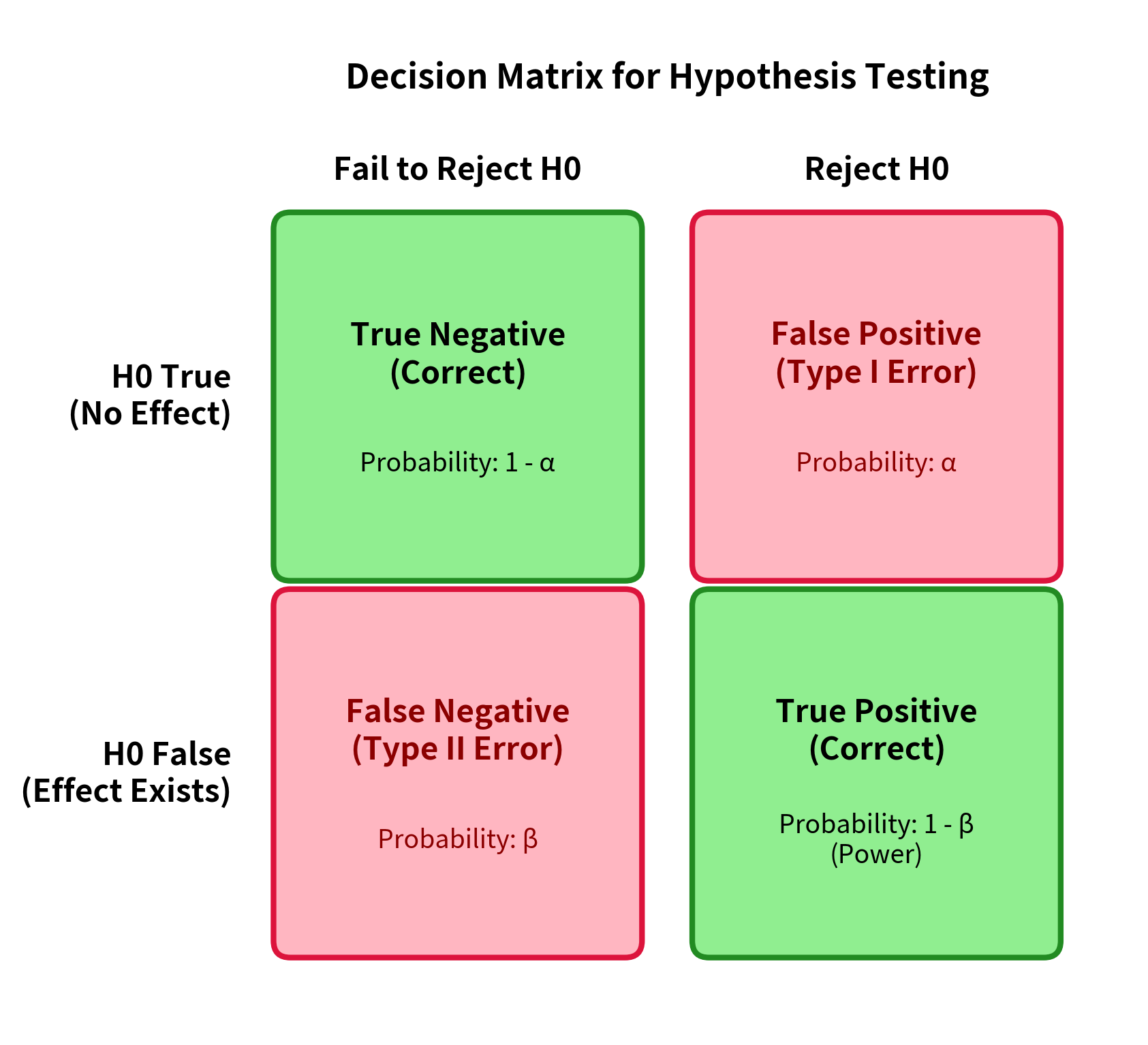
When we conduct a hypothesis test, we are making a binary decision: reject the null hypothesis or fail to reject it. Reality also has two states: either the null hypothesis is true, or it is false. This creates a 2×2 matrix of possible outcomes.

Out[2]:

Visualization

A 2x2 matrix showing the four possible outcomes of hypothesis testing decisions. — The four possible outcomes when making a decision based on a hypothesis test. Correct decisions occur when our conclusion matches reality. Errors occur when they do not. Type I errors (false positives) happen when we reject a true null hypothesis. Type II errors (false negatives) happen when we fail to reject a false null hypothesis.

Let's define these four outcomes precisely:

True Negative: The null hypothesis is true (no effect exists), and we correctly fail to reject it. This is a correct decision.
True Positive: The null hypothesis is false (an effect exists), and we correctly reject it. This is a correct decision, and its probability is called power.
Type I Error (False Positive): The null hypothesis is true (no effect exists), but we incorrectly reject it. We claim to have found something that isn't there.
Type II Error (False Negative): The null hypothesis is false (an effect exists), but we fail to reject it. We miss a real effect that is actually there.

Type I Errors: The False AlarmLink Copied

A Type I error occurs when you reject a true null hypothesis. In plain language: you conclude that something interesting is happening when, in reality, nothing is going on. You've raised a false alarm.

The Probability of Type I Error: αLink Copied

The probability of a Type I error is denoted by the Greek letter alpha (α), and it equals the significance level you choose for your test. When you set α = 0.05, you are accepting a 5% probability of falsely rejecting the null hypothesis when it is true.

Mathematically:

\alpha = P(\text{Reject } H_0 \mid H_0 \text{ is true})

This is a conditional probability: the probability of rejecting the null hypothesis, given that the null hypothesis is actually true. It represents the false positive rate of your test.

Why α Equals the Significance LevelLink Copied

To understand why α equals our chosen significance level, recall how hypothesis testing works. We:

Assume the null hypothesis is true
Calculate the sampling distribution of our test statistic under this assumption
Determine what values of the test statistic would be "extreme enough" to reject $H_0$
The significance level is precisely the probability of observing such extreme values when $H_0$ is true

For a two-tailed z-test with α = 0.05:

\alpha = P(|Z| > z_{\alpha/2} \mid H_0) = P(Z < -1.96) + P(Z > 1.96) = 0.025 + 0.025 = 0.05

Out[3]:

Visualization

Normal distribution with shaded rejection regions in both tails. — The null distribution showing regions where we would reject H₀. The shaded areas in the tails represent the probability of a Type I error (α). When we set α = 0.05, we reject H₀ if our test statistic falls in either tail beyond ±1.96. These are precisely the values that would occur only 5% of the time if H₀ were true.

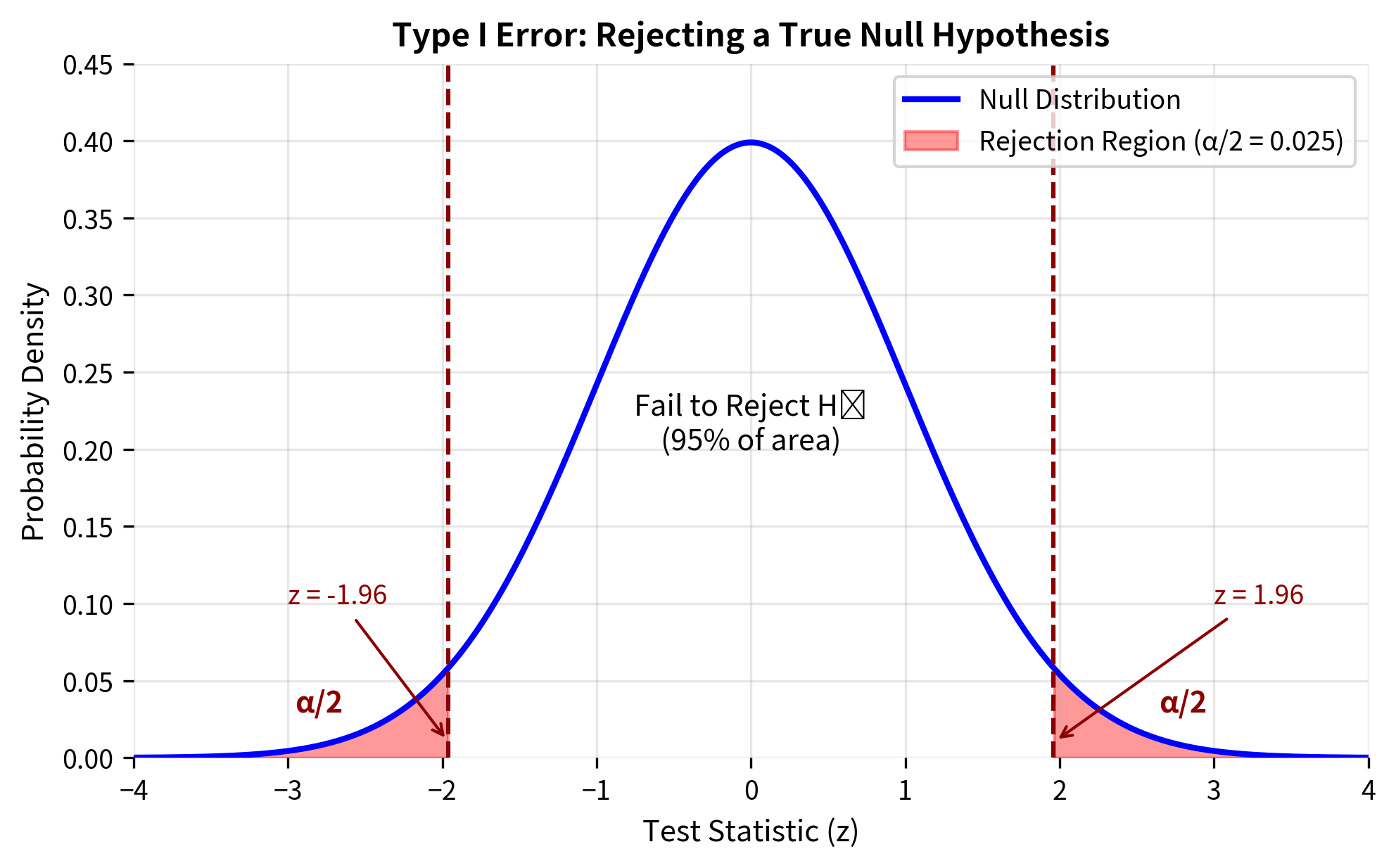
The Key Insight: You Control αLink Copied

Unlike many other aspects of hypothesis testing, the significance level α is under your direct control. You choose it before conducting the test, based on the consequences of false positives in your specific context.

The conventional choice of α = 0.05 is just that, a convention. It was popularized by Ronald Fisher in the early 20th century as a reasonable default, but it is not a universal law. Different contexts warrant different choices:

Context	Typical α	Rationale
Exploratory research	0.10	Missing effects is costly; expect replication
Standard scientific research	0.05	Convention balancing Type I and II errors
Confirmatory/regulatory	0.01	False positives have serious consequences
Particle physics discoveries	~0.0000003 (5σ)	Extraordinary claims require extraordinary evidence
Genome-wide association	5 × 10⁻⁸	Multiple testing across millions of variants

Real-World Consequences of Type I ErrorsLink Copied

Type I errors can have serious consequences across many domains:

Medical diagnosis: A healthy patient is told they have cancer. This causes severe psychological distress, leads to invasive follow-up procedures (biopsies, additional imaging), and may result in unnecessary treatment with harmful side effects.

Criminal justice: An innocent person is convicted of a crime. This is the scenario our legal systems are designed to prevent: the presumption of innocence exists precisely because Type I errors (convicting the innocent) are considered worse than Type II errors (acquitting the guilty).

Drug approval: The FDA approves a drug that is actually no better than placebo. Patients take an ineffective medication, potentially experiencing side effects without any benefit, while being denied treatments that might actually work.

A/B testing: A company deploys a new website design based on a "significant" result that was actually just noise. Engineering resources are wasted, and if the change is actually harmful, user experience suffers.

Scientific research: A researcher publishes a "discovery" that is just a statistical fluke. Other researchers waste time and resources trying to replicate or build on the finding. The scientific literature becomes polluted with false results.

Type II Errors: The Missed DiscoveryLink Copied

A Type II error occurs when you fail to reject a false null hypothesis. In plain language: a real effect exists, but your test fails to detect it. You've missed a genuine discovery.

The Probability of Type II Error: βLink Copied

The probability of a Type II error is denoted by the Greek letter beta (β):

\beta = P(\text{Fail to reject } H_0 \mid H_0 \text{ is false})

This is also a conditional probability: the probability of not rejecting the null hypothesis, given that it is actually false.

Computing β: The MathematicsLink Copied

Unlike α, which you simply choose, β must be calculated based on several factors. The calculation requires specifying an alternative hypothesis: you need to know what the true state of the world is to compute the probability of missing it.

Let's work through the mathematics for a one-sample z-test. Suppose:

Null hypothesis: $H_0: \mu = \mu_0$
True population mean: $\mu = \mu_1$ (where $\mu_1 \neq \mu_0$ )
Known population standard deviation: $\sigma$
Sample size: $n$
Significance level: $\alpha$ (two-tailed test)

Step 1: Find the critical values under $H_0$

Under the null hypothesis, the test statistic $Z = \frac{\bar{X} - \mu_0}{\sigma / \sqrt{n}}$ follows a standard normal distribution. The critical values for a two-tailed test at significance level α are:

z_{\text{crit}} = \pm z_{\alpha/2}

For α = 0.05: $z_{\text{crit}} = \pm 1.96$

Step 2: Convert critical z-values to critical sample means

We reject $H_0$ if $\bar{X}$ falls outside the interval:

\bar{X}_{\text{lower}} = \mu_0 - z_{\alpha/2} \cdot \frac{\sigma}{\sqrt{n}}

\bar{X}_{\text{upper}} = \mu_0 + z_{\alpha/2} \cdot \frac{\sigma}{\sqrt{n}}

Step 3: Calculate β under the alternative

A Type II error occurs when $\bar{X}$ falls in the "fail to reject" region even though the true mean is $\mu_1$ . Under the alternative:

\bar{X} \sim N\left(\mu_1, \frac{\sigma^2}{n}\right)

The probability of not rejecting $H_0$ is:

\beta = P\left(\bar{X}_{\text{lower}} < \bar{X} < \bar{X}_{\text{upper}} \mid \mu = \mu_1\right)

Standardizing using the true mean $\mu_1$ :

\beta = \Phi\left(\frac{\bar{X}_{\text{upper}} - \mu_1}{\sigma/\sqrt{n}}\right) - \Phi\left(\frac{\bar{X}_{\text{lower}} - \mu_1}{\sigma/\sqrt{n}}\right)

where $\Phi$ is the standard normal CDF.

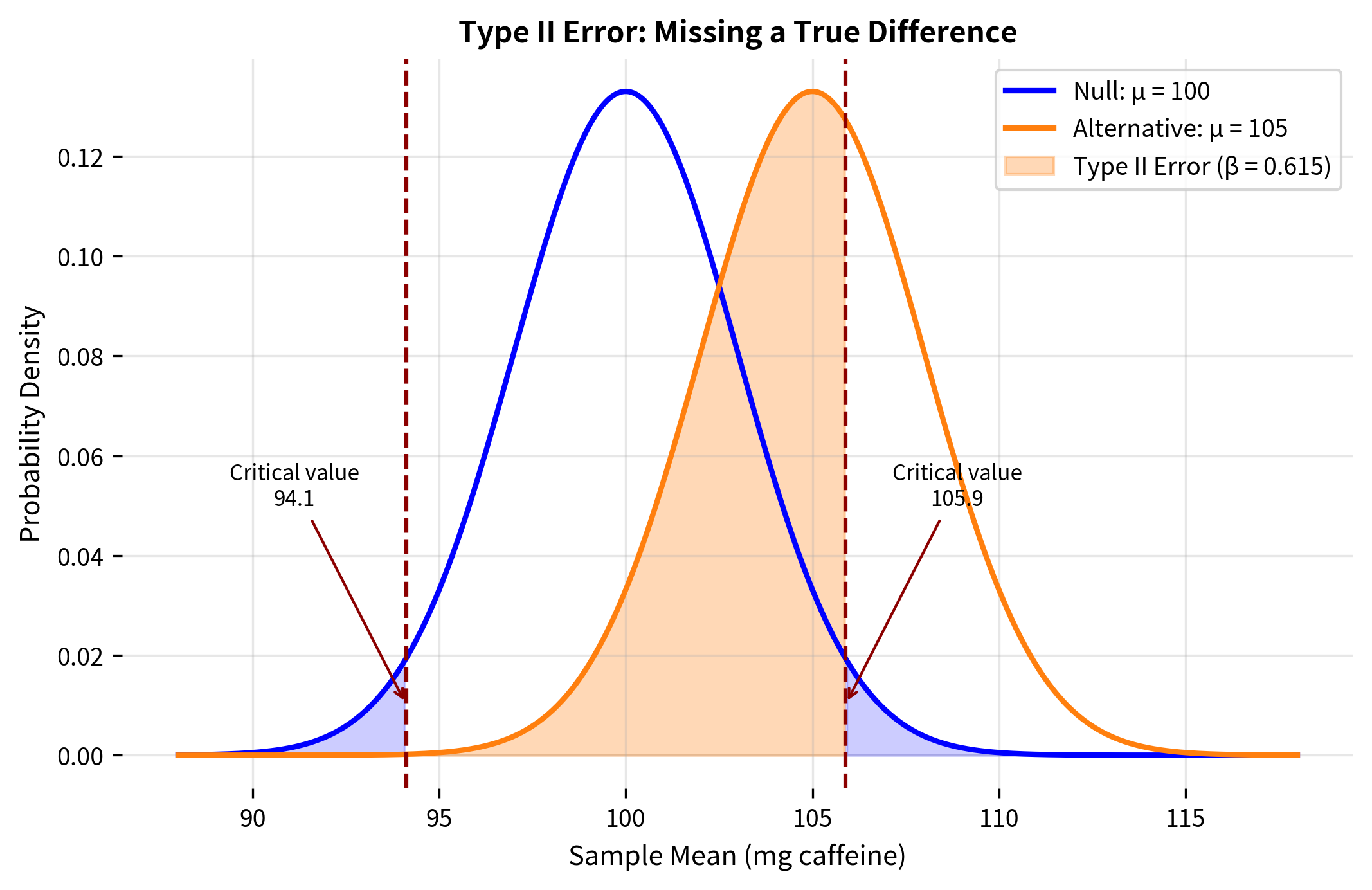
Worked Example: Calculating βLink Copied

Let's calculate β for a concrete scenario.

Scenario: A coffee company claims their beans have a mean caffeine content of 100 mg per cup ( $H_0: \mu = 100$ ). A consumer group suspects the true content is 105 mg ( $H_1: \mu = 105$ ). They plan to test 25 cups, and caffeine content is known to have σ = 15 mg.

In[4]:

Code

import numpy as np
from scipy import stats

# Parameters
mu_0 = 100  # Null hypothesis mean
mu_1 = 105  # True mean (alternative)
sigma = 15  # Population standard deviation
n = 25  # Sample size
alpha = 0.05  # Significance level

# Standard error
se = sigma / np.sqrt(n)
print(f"Standard error: σ/√n = {sigma}/√{n} = {se:.2f}")

# Critical values for the sample mean (two-tailed test)
z_crit = stats.norm.ppf(1 - alpha / 2)
x_lower = mu_0 - z_crit * se
x_upper = mu_0 + z_crit * se
print(f"\nCritical z-value: ±{z_crit:.3f}")
print(f"Fail to reject H₀ if: {x_lower:.2f} < X̄ < {x_upper:.2f}")

# Calculate β: P(fail to reject | H₁ is true)
# This is P(x_lower < X̄ < x_upper) when X̄ ~ N(mu_1, se²)
beta = stats.norm.cdf(x_upper, loc=mu_1, scale=se) - stats.norm.cdf(
    x_lower, loc=mu_1, scale=se
)
print(f"\nType II error probability: β = {beta:.4f} ({beta * 100:.1f}%)")
print(f"Power (1 - β) = {1 - beta:.4f} ({(1 - beta) * 100:.1f}%)")

import numpy as np
from scipy import stats

# Parameters
mu_0 = 100  # Null hypothesis mean
mu_1 = 105  # True mean (alternative)
sigma = 15  # Population standard deviation
n = 25  # Sample size
alpha = 0.05  # Significance level

# Standard error
se = sigma / np.sqrt(n)
print(f"Standard error: σ/√n = {sigma}/√{n} = {se:.2f}")

# Critical values for the sample mean (two-tailed test)
z_crit = stats.norm.ppf(1 - alpha / 2)
x_lower = mu_0 - z_crit * se
x_upper = mu_0 + z_crit * se
print(f"\nCritical z-value: ±{z_crit:.3f}")
print(f"Fail to reject H₀ if: {x_lower:.2f} < X̄ < {x_upper:.2f}")

# Calculate β: P(fail to reject | H₁ is true)
# This is P(x_lower < X̄ < x_upper) when X̄ ~ N(mu_1, se²)
beta = stats.norm.cdf(x_upper, loc=mu_1, scale=se) - stats.norm.cdf(
    x_lower, loc=mu_1, scale=se
)
print(f"\nType II error probability: β = {beta:.4f} ({beta * 100:.1f}%)")
print(f"Power (1 - β) = {1 - beta:.4f} ({(1 - beta) * 100:.1f}%)")

Out[4]:

Console

Standard error: σ/√n = 15/√25 = 3.00

Critical z-value: ±1.960
Fail to reject H₀ if: 94.12 < X̄ < 105.88

Type II error probability: β = 0.6152 (61.5%)
Power (1 - β) = 0.3848 (38.5%)

Let's visualize what's happening:

Out[5]:

Visualization

Two overlapping normal distributions showing the relationship between null and alternative hypotheses and the Type II error region. — Visualization of Type II error. The blue distribution shows the sampling distribution under the null hypothesis (μ = 100). The orange distribution shows the sampling distribution under the true alternative (μ = 105). The vertical dashed lines mark the critical values. The orange shaded area represents β: the probability that our sample mean falls in the ''fail to reject'' region even when the true mean is 105.

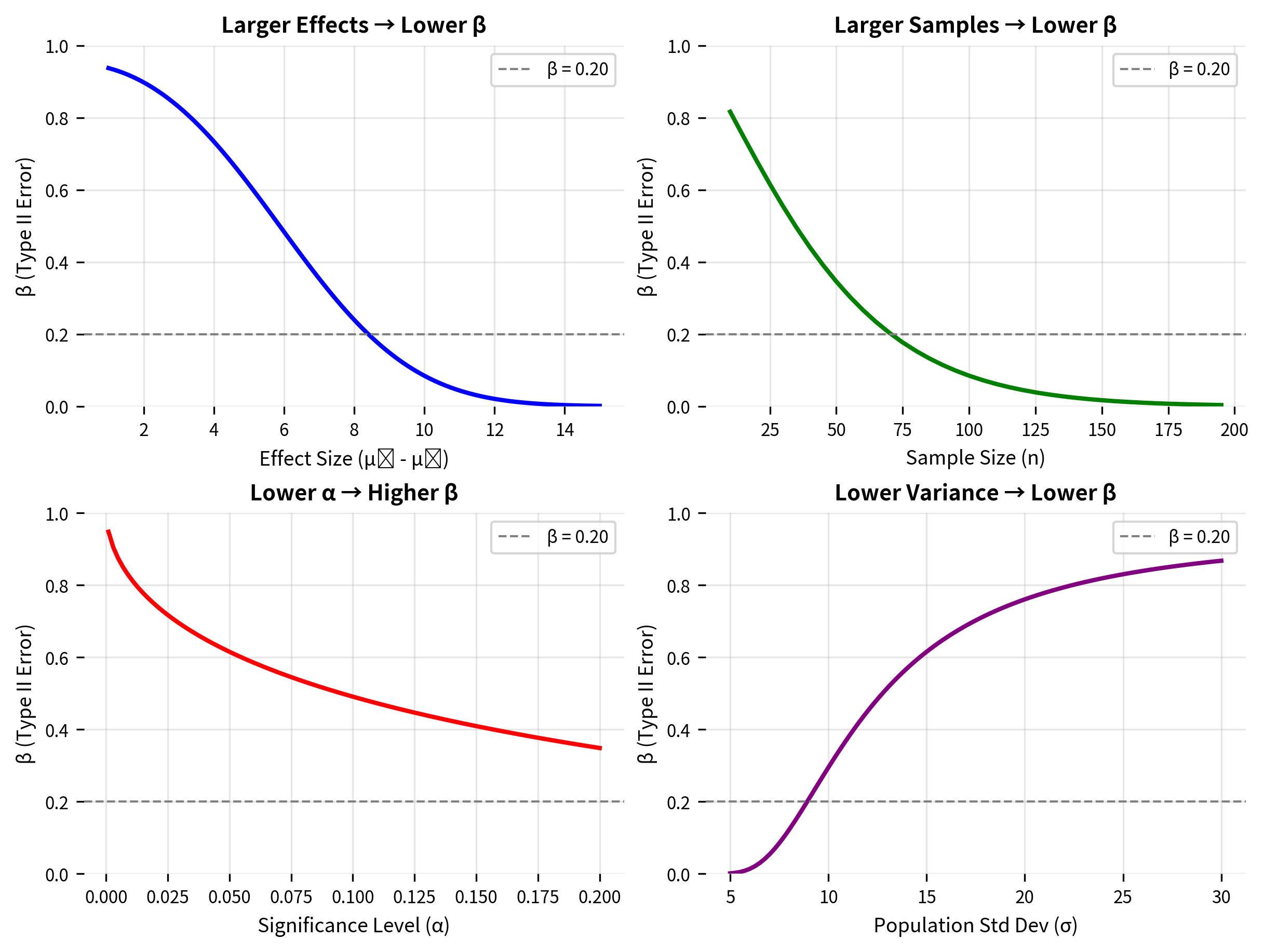
What Determines β?Link Copied

The Type II error probability depends on four interrelated factors:

1. Effect size: The larger the true effect (the distance between $\mu_0$ and $\mu_1$ ), the smaller β becomes. Larger effects are easier to detect because the alternative distribution is further from the null distribution.

2. Sample size: Larger samples decrease β. More data reduces the standard error $\sigma/\sqrt{n}$ , making both distributions narrower and easier to distinguish.

3. Significance level: Lower α means higher β, all else equal. Making it harder to reject $H_0$ (requiring more extreme evidence) also makes it harder to detect true effects.

4. Population variability: Lower population variance (smaller σ) decreases β. Less noise means the signal is easier to detect.

Out[6]:

Visualization

Four panel plot showing how effect size, sample size, significance level, and population variance affect beta. — How different factors affect Type II error probability (β). Top-left: Larger effect sizes reduce β. Top-right: Larger sample sizes reduce β. Bottom-left: Lower significance levels increase β. Bottom-right: Lower population variance reduces β. The conventional target of β = 0.20 (80% power) is shown as a dashed line.

Real-World Consequences of Type II ErrorsLink Copied

Type II errors represent missed opportunities and can have serious consequences:

Medical diagnosis: A patient with early-stage cancer is told their screening test is negative. The cancer continues to grow undetected, potentially reaching a stage where treatment is less effective.

Drug development: A pharmaceutical company abandons a drug that would actually be effective because their clinical trial failed to show a statistically significant benefit. Patients are deprived of a treatment that could help them.

Safety testing: An engineer fails to detect that a structural component is weaker than specifications require. The component is used in construction, potentially leading to failure under stress.

Criminal justice: A guilty person is acquitted due to insufficient evidence. While this is preferred to convicting the innocent, it still represents a failure of the justice system to hold offenders accountable.

Research: A scientist fails to detect a genuine relationship in their data. The discovery is delayed or never made, slowing scientific progress.

Statistical Power: 1 - βLink Copied

Statistical power is defined as $1 - \beta$ : the probability of correctly rejecting a false null hypothesis. If β is the probability of a Type II error (missing a real effect), then power is the probability of detecting that real effect.

\text{Power} = 1 - \beta = P(\text{Reject } H_0 \mid H_0 \text{ is false})

Why Power MattersLink Copied

Power tells you how sensitive your study is. If a genuine effect exists, power gives the probability that your study will find it:

80% power: 80% chance of detecting a true effect, 20% chance of missing it
50% power: Essentially a coin flip: you're as likely to miss the effect as to find it
20% power: You'll miss the effect 80% of the time: your study is almost useless

The conventional target is 80% power (β = 0.20). This means accepting a 1-in-5 chance of missing a real effect, which is considered an acceptable tradeoff in most research contexts. Some fields, particularly confirmatory research or high-stakes decisions, target 90% power.

Power CurvesLink Copied

A power curve shows how power varies with effect size for a given sample size and significance level. These curves are essential for understanding what effects your study can detect.

Out[7]:

Visualization

Line plot showing power curves that increase with effect size, with different curves for different sample sizes. — Power curves showing the probability of detecting an effect as a function of effect size (Cohen's d) for different sample sizes. The dashed horizontal line marks 80% power, the conventional target. Larger samples allow detection of smaller effects. With n = 10, you need a large effect (d ≈ 1.0) to reach 80% power. With n = 200, even a small effect (d ≈ 0.2) can be detected with high probability.

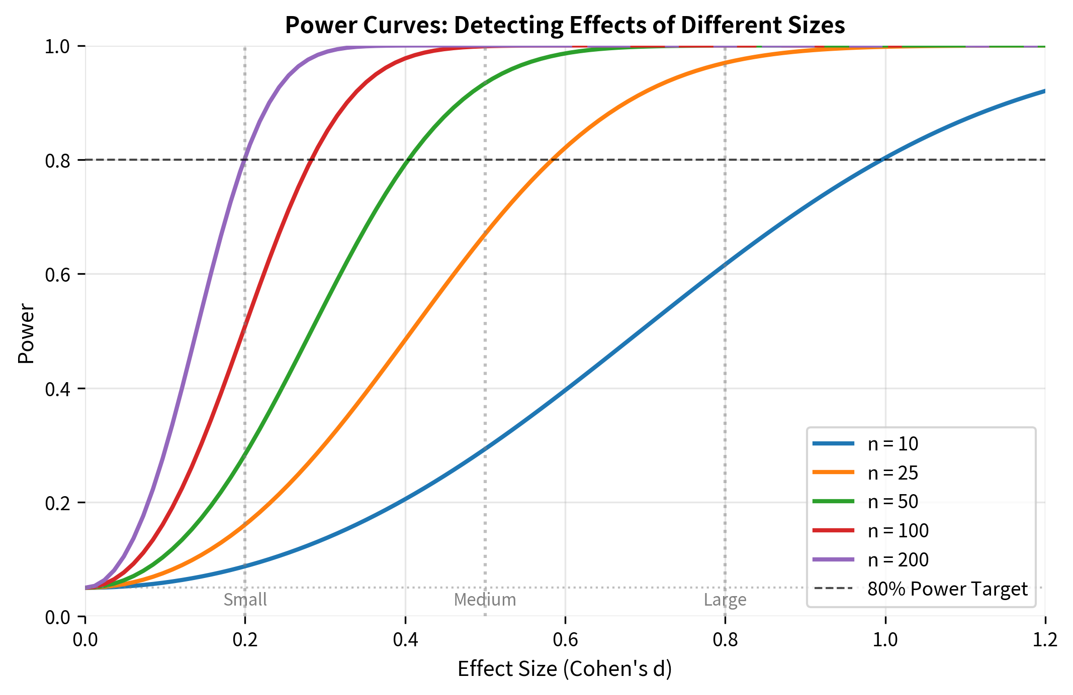
The Problem of Underpowered StudiesLink Copied

Underpowered studies are one of the most serious problems in research. When a study lacks sufficient power:

True effects are missed: The study is likely to produce a non-significant result even when a real effect exists.
Significant results are exaggerated: If an underpowered study does find significance, the effect size estimate is likely to be inflated (the "winner's curse").
Non-significant results are misinterpreted: Researchers may incorrectly conclude that "there is no effect" when the study simply lacked the power to detect it.
Resources are wasted: Time, money, and participant effort go into studies that cannot answer the research question.
Publication bias is amplified: Only the "lucky" underpowered studies that happen to achieve significance get published, leading to a distorted literature.

In[8]:

Code

import numpy as np
from scipy import stats

np.random.seed(42)

# Simulate an underpowered study
# True effect: d = 0.3 (small effect)
# Sample size: n = 20 per group (typical for many studies)

n_simulations = 10000
n_per_group = 20
true_effect = 0.3  # Cohen's d
alpha = 0.05

significant_count = 0
significant_effects = []

for _ in range(n_simulations):
    # Generate data from two populations with a true difference
    group1 = np.random.normal(0, 1, n_per_group)
    group2 = np.random.normal(true_effect, 1, n_per_group)

    # Conduct t-test
    t_stat, p_value = stats.ttest_ind(group2, group1)

    if p_value < alpha:
        significant_count += 1
        # Calculate observed effect size
        pooled_std = np.sqrt(
            (np.var(group1, ddof=1) + np.var(group2, ddof=1)) / 2
        )
        observed_d = (np.mean(group2) - np.mean(group1)) / pooled_std
        significant_effects.append(observed_d)

power = significant_count / n_simulations
print(f"True effect size: d = {true_effect}")
print(f"Sample size: n = {n_per_group} per group")
print(f"Simulated power: {power:.1%}")
print(f"\nOf {n_simulations:,} studies:")
print(f"  - {significant_count:,} achieved p < 0.05")
print(f"  - {n_simulations - significant_count:,} failed to detect the effect")

if significant_effects:
    print("\nAmong significant results:")
    print(f"  - Mean observed effect: d = {np.mean(significant_effects):.3f}")
    print(
        f"  - This is {np.mean(significant_effects) / true_effect:.1f}x the true effect!"
    )

import numpy as np
from scipy import stats

np.random.seed(42)

# Simulate an underpowered study
# True effect: d = 0.3 (small effect)
# Sample size: n = 20 per group (typical for many studies)

n_simulations = 10000
n_per_group = 20
true_effect = 0.3  # Cohen's d
alpha = 0.05

significant_count = 0
significant_effects = []

for _ in range(n_simulations):
    # Generate data from two populations with a true difference
    group1 = np.random.normal(0, 1, n_per_group)
    group2 = np.random.normal(true_effect, 1, n_per_group)

    # Conduct t-test
    t_stat, p_value = stats.ttest_ind(group2, group1)

    if p_value < alpha:
        significant_count += 1
        # Calculate observed effect size
        pooled_std = np.sqrt(
            (np.var(group1, ddof=1) + np.var(group2, ddof=1)) / 2
        )
        observed_d = (np.mean(group2) - np.mean(group1)) / pooled_std
        significant_effects.append(observed_d)

power = significant_count / n_simulations
print(f"True effect size: d = {true_effect}")
print(f"Sample size: n = {n_per_group} per group")
print(f"Simulated power: {power:.1%}")
print(f"\nOf {n_simulations:,} studies:")
print(f"  - {significant_count:,} achieved p < 0.05")
print(f"  - {n_simulations - significant_count:,} failed to detect the effect")

if significant_effects:
    print("\nAmong significant results:")
    print(f"  - Mean observed effect: d = {np.mean(significant_effects):.3f}")
    print(
        f"  - This is {np.mean(significant_effects) / true_effect:.1f}x the true effect!"
    )

Out[8]:

Console

True effect size: d = 0.3
Sample size: n = 20 per group
Simulated power: 15.6%

Of 10,000 studies:
  - 1,559 achieved p < 0.05
  - 8,441 failed to detect the effect

Among significant results:
  - Mean observed effect: d = 0.793
  - This is 2.6x the true effect!

This simulation demonstrates the winner's curse: when underpowered studies do achieve significance, they systematically overestimate the true effect size. This happens because only the "lucky" samples, those with upward random fluctuations, cross the significance threshold.

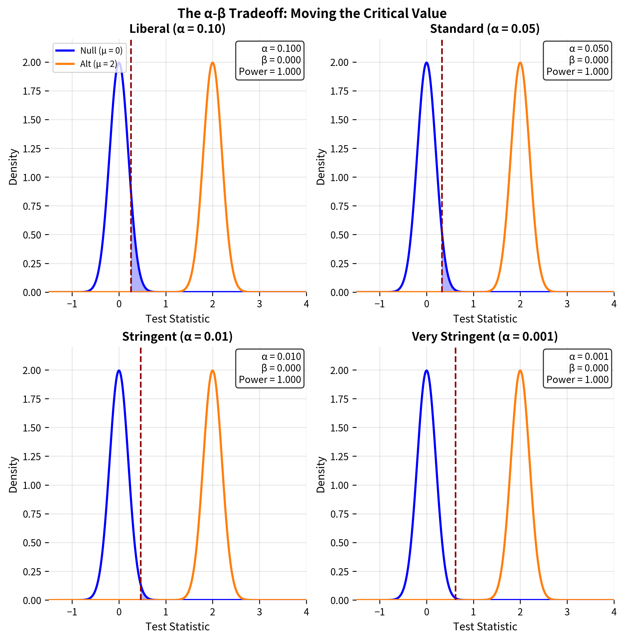
The Fundamental TradeoffLink Copied

For a fixed sample size, there is an inevitable tradeoff between Type I and Type II errors. Decreasing α (being more stringent about false positives) necessarily increases β (making false negatives more likely), and vice versa.

This tradeoff is best visualized by showing both distributions, the null and the alternative, and seeing how the critical value divides the space.

Out[9]:

Visualization

Managing the TradeoffLink Copied

Given this tradeoff, how should you balance Type I and Type II errors? The answer depends on the relative costs of each error type in your specific context.

Framework for Choosing α:

Consider what happens if you make each type of error:

If Type I Error is...	And Type II Error is...	Then...
Very costly	Less costly	Use lower α (0.01 or lower)
Less costly	Very costly	Use higher α (0.10) and ensure adequate power
Equally costly	Equally costly	Use conventional α (0.05)

Examples of Context-Dependent Decisions:

Criminal trial: Type I error (convicting innocent) is considered much worse than Type II error (acquitting guilty). This is why "beyond reasonable doubt" sets a very high bar, effectively using a very low α.
Medical screening: For a deadly but treatable disease, Type II error (missing cases) may be worse than Type I error (false alarms that lead to follow-up testing). A higher α might be appropriate.
Drug approval: Both errors are costly: approving ineffective drugs (Type I) wastes resources and exposes patients to side effects, while rejecting effective drugs (Type II) denies patients beneficial treatments. The FDA's approach is to use stringent α but also require adequate sample sizes for power.
Particle physics: Claiming a new particle discovery that is actually noise would be extremely embarrassing and wasteful. The 5-sigma standard (α ≈ 3 × 10⁻⁷) reflects the high cost of Type I errors in this field.

Putting It All Together: A Worked ExampleLink Copied

Let's work through a complete example that ties together all the concepts.

Scenario: A pharmaceutical company is testing whether a new drug reduces blood pressure more than the current standard treatment. They need to design a study that balances both error types appropriately.

In[10]:

Code

import numpy as np
from scipy import stats

# Study parameters
# Current treatment: mean reduction of 10 mmHg
# New drug: suspected to reduce by 13 mmHg (3 mmHg improvement)
# Standard deviation: 8 mmHg (from previous studies)

mu_0 = 10  # Effect of current treatment (null: new drug is same)
mu_1 = 13  # Expected effect of new drug
sigma = 8  # Population standard deviation
effect = mu_1 - mu_0  # Expected improvement

print("=== Study Design Analysis ===\n")
print(f"Null hypothesis: New drug effect = {mu_0} mmHg (same as current)")
print(f"Alternative: New drug effect = {mu_1} mmHg")
print(f"Expected improvement: {effect} mmHg")
print(f"Population SD: {sigma} mmHg")

# Analysis with different sample sizes
print("\n--- Power Analysis ---")
print(f"{'n':<8} {'SE':<8} {'β':<10} {'Power':<10}")
print("-" * 40)

for n in [25, 50, 100, 150, 200]:
    se = sigma / np.sqrt(n)
    z_crit = stats.norm.ppf(0.975)  # Two-tailed, α = 0.05

    # Critical values for sample mean
    x_lower = mu_0 - z_crit * se
    x_upper = mu_0 + z_crit * se

    # Beta under alternative (focusing on upper tail since we expect mu_1 > mu_0)
    beta = stats.norm.cdf(x_upper, loc=mu_1, scale=se) - stats.norm.cdf(
        x_lower, loc=mu_1, scale=se
    )
    power = 1 - beta

    print(f"{n:<8} {se:<8.2f} {beta:<10.4f} {power:<10.1%}")

import numpy as np
from scipy import stats

# Study parameters
# Current treatment: mean reduction of 10 mmHg
# New drug: suspected to reduce by 13 mmHg (3 mmHg improvement)
# Standard deviation: 8 mmHg (from previous studies)

mu_0 = 10  # Effect of current treatment (null: new drug is same)
mu_1 = 13  # Expected effect of new drug
sigma = 8  # Population standard deviation
effect = mu_1 - mu_0  # Expected improvement

print("=== Study Design Analysis ===\n")
print(f"Null hypothesis: New drug effect = {mu_0} mmHg (same as current)")
print(f"Alternative: New drug effect = {mu_1} mmHg")
print(f"Expected improvement: {effect} mmHg")
print(f"Population SD: {sigma} mmHg")

# Analysis with different sample sizes
print("\n--- Power Analysis ---")
print(f"{'n':<8} {'SE':<8} {'β':<10} {'Power':<10}")
print("-" * 40)

for n in [25, 50, 100, 150, 200]:
    se = sigma / np.sqrt(n)
    z_crit = stats.norm.ppf(0.975)  # Two-tailed, α = 0.05

    # Critical values for sample mean
    x_lower = mu_0 - z_crit * se
    x_upper = mu_0 + z_crit * se

    # Beta under alternative (focusing on upper tail since we expect mu_1 > mu_0)
    beta = stats.norm.cdf(x_upper, loc=mu_1, scale=se) - stats.norm.cdf(
        x_lower, loc=mu_1, scale=se
    )
    power = 1 - beta

    print(f"{n:<8} {se:<8.2f} {beta:<10.4f} {power:<10.1%}")

Out[10]:

Console

=== Study Design Analysis ===

Null hypothesis: New drug effect = 10 mmHg (same as current)
Alternative: New drug effect = 13 mmHg
Expected improvement: 3 mmHg
Population SD: 8 mmHg

--- Power Analysis ---
n        SE       β          Power     
----------------------------------------
25       1.60     0.5338     46.6%     
50       1.13     0.2446     75.5%     
100      0.80     0.0367     96.3%     
150      0.65     0.0042     99.6%     
200      0.57     0.0004     100.0%

Out[11]:

Visualization

Line plot showing power increasing with sample size, with 80% power marked. — Power analysis for the blood pressure drug study. The plot shows how power increases with sample size. With α = 0.05 and an expected 3 mmHg improvement (σ = 8 mmHg), approximately 100 patients per group are needed to achieve 80% power. Recruiting fewer patients risks missing a genuine clinical benefit.

Decision Framework for the ExampleLink Copied

Based on this analysis, the pharmaceutical company can make an informed decision:

In[12]:

Code

# Summary of study design options

print("=== Study Design Decision Framework ===\n")

options = [
    {
        "n": 50,
        "power": 0.56,
        "cost": "Low",
        "risk": "High (44% chance of missing a real benefit)",
    },
    {
        "n": 100,
        "power": 0.80,
        "cost": "Medium",
        "risk": "Moderate (20% chance of missing a real benefit)",
    },
    {
        "n": 150,
        "power": 0.91,
        "cost": "High",
        "risk": "Low (9% chance of missing a real benefit)",
    },
]

print("Option Analysis:")
print("-" * 70)
for opt in options:
    print(f"\nn = {opt['n']} patients per group:")
    print(f"  Power: {opt['power']:.0%}")
    print(f"  Cost: {opt['cost']}")
    print(f"  Risk: {opt['risk']}")

print("\n" + "=" * 70)
print("\nRecommendation: n = 100 per group")
print("  - Achieves conventional 80% power target")
print("  - Balances cost with acceptable Type II error risk")
print("  - If budget allows, n = 150 provides additional safety margin")

# Summary of study design options

print("=== Study Design Decision Framework ===\n")

options = [
    {
        "n": 50,
        "power": 0.56,
        "cost": "Low",
        "risk": "High (44% chance of missing a real benefit)",
    },
    {
        "n": 100,
        "power": 0.80,
        "cost": "Medium",
        "risk": "Moderate (20% chance of missing a real benefit)",
    },
    {
        "n": 150,
        "power": 0.91,
        "cost": "High",
        "risk": "Low (9% chance of missing a real benefit)",
    },
]

print("Option Analysis:")
print("-" * 70)
for opt in options:
    print(f"\nn = {opt['n']} patients per group:")
    print(f"  Power: {opt['power']:.0%}")
    print(f"  Cost: {opt['cost']}")
    print(f"  Risk: {opt['risk']}")

print("\n" + "=" * 70)
print("\nRecommendation: n = 100 per group")
print("  - Achieves conventional 80% power target")
print("  - Balances cost with acceptable Type II error risk")
print("  - If budget allows, n = 150 provides additional safety margin")

Out[12]:

Console

=== Study Design Decision Framework ===

Option Analysis:
----------------------------------------------------------------------

n = 50 patients per group:
  Power: 56%
  Cost: Low
  Risk: High (44% chance of missing a real benefit)

n = 100 patients per group:
  Power: 80%
  Cost: Medium
  Risk: Moderate (20% chance of missing a real benefit)

n = 150 patients per group:
  Power: 91%
  Cost: High
  Risk: Low (9% chance of missing a real benefit)

======================================================================

Recommendation: n = 100 per group
  - Achieves conventional 80% power target
  - Balances cost with acceptable Type II error risk
  - If budget allows, n = 150 provides additional safety margin

SummaryLink Copied

Type I and Type II errors are the two ways hypothesis tests can fail. Understanding them is essential for designing studies and interpreting results:

Type I Error (α): Rejecting a true null hypothesis, a false positive. You conclude an effect exists when it doesn't.

Probability equals your chosen significance level
You control α directly by your choice of significance threshold
Consequences: wasted resources, false claims, harm from unnecessary interventions

Type II Error (β): Failing to reject a false null hypothesis, a false negative. You miss a real effect.

Probability depends on effect size, sample size, significance level, and population variance
You influence β through study design, primarily sample size
Consequences: missed discoveries, failed treatments, wasted research effort

Power (1 - β): The probability of correctly detecting a true effect.

Conventional target: 80% (β = 0.20)
Higher power requires larger samples, larger effects, or higher α
Underpowered studies are one of the most serious problems in research

The Fundamental Tradeoff: For a fixed sample size, decreasing α increases β. The only way to reduce both simultaneously is to increase the sample size.

The key insight is that these error rates are not just abstract probabilities: they have real consequences for patients, businesses, and scientific progress. Thoughtful study design requires explicitly considering these tradeoffs in the context of your specific application.

What's NextLink Copied

Understanding error types prepares you for power analysis and sample size determination. In the next section, you'll learn how to calculate the sample size needed to detect effects of a given size with a specified probability. This involves:

Setting power targets based on the consequences of Type II errors
Calculating minimum detectable effects for given sample sizes
Understanding the relationship between effect size, sample size, and power
Using power analysis software and formulas

You'll also explore effect sizes in depth: standardized measures of the magnitude of effects that are independent of sample size. Effect sizes are essential for interpreting results and for meta-analysis, where results from multiple studies are combined. Finally, you'll learn about multiple comparisons, where conducting many tests inflates the overall Type I error rate and requires special correction methods.

These concepts build directly on the error framework you've learned here. Every statistical decision involves weighing the risks of Type I and Type II errors—the tools in upcoming sections will help you make these decisions systematically.

QuizLink Copied

Ready to test your understanding? Take this quick quiz to reinforce what you've learned about Type I and Type II errors.

Loading component...

Comments

Back to Machine Learning from Scratch

Previous Chapter

ANOVA (Analysis of Variance)

Next Chapter

Sample Size, Minimum Detectable Effect, and Power

Reference

BIBTEXAcademic

@misc{typeiandtypeiierrorsfalsepositivesfalsenegativesstatisticalpower, author = {Michael Brenndoerfer}, title = {Type I and Type II Errors: False Positives, False Negatives & Statistical Power}, year = {2026}, url = {https://mbrenndoerfer.com/writing/type-i-type-ii-errors-false-positives-false-negatives-statistical-power}, organization = {mbrenndoerfer.com}, note = {Accessed: 2025-01-01} }

APAAcademic

Michael Brenndoerfer (2026). Type I and Type II Errors: False Positives, False Negatives & Statistical Power. Retrieved from https://mbrenndoerfer.com/writing/type-i-type-ii-errors-false-positives-false-negatives-statistical-power

MLAAcademic

Michael Brenndoerfer. "Type I and Type II Errors: False Positives, False Negatives & Statistical Power." 2026. Web. today. <https://mbrenndoerfer.com/writing/type-i-type-ii-errors-false-positives-false-negatives-statistical-power>.

CHICAGOAcademic

Michael Brenndoerfer. "Type I and Type II Errors: False Positives, False Negatives & Statistical Power." Accessed today. https://mbrenndoerfer.com/writing/type-i-type-ii-errors-false-positives-false-negatives-statistical-power.

HARVARDAcademic

Michael Brenndoerfer (2026) 'Type I and Type II Errors: False Positives, False Negatives & Statistical Power'. Available at: https://mbrenndoerfer.com/writing/type-i-type-ii-errors-false-positives-false-negatives-statistical-power (Accessed: today).

SimpleBasic

Michael Brenndoerfer (2026). Type I and Type II Errors: False Positives, False Negatives & Statistical Power. https://mbrenndoerfer.com/writing/type-i-type-ii-errors-false-positives-false-negatives-statistical-power

Direct link:

https://mbrenndoerfer.com/writing/type-i-type-ii-errors-false-positives-false-negatives-statistical-power

About the author: Michael Brenndoerfer

All opinions expressed here are my own and do not reflect the views of my employer.

Michael currently works as an Associate Director of Data Science at EQT Partners in Singapore, leading AI and data initiatives across private capital investments.

With over a decade of experience spanning private equity, management consulting, and software engineering, he specializes in building and scaling analytics capabilities from the ground up. He has published research in leading AI conferences and holds expertise in machine learning, natural language processing, and value creation through data.

View Full Resume Publications Contact Books

Type I and Type II Errors: False Positives, False Negatives & Statistical Power

Type I and Type II ErrorsLink Copied

The Two Ways Tests Can FailLink Copied

Type I Errors: The False AlarmLink Copied

The Probability of Type I Error: αLink Copied

Why α Equals the Significance LevelLink Copied

The Key Insight: You Control αLink Copied

Real-World Consequences of Type I ErrorsLink Copied

Type II Errors: The Missed DiscoveryLink Copied

The Probability of Type II Error: βLink Copied

Computing β: The MathematicsLink Copied

Worked Example: Calculating βLink Copied

What Determines β?Link Copied

Real-World Consequences of Type II ErrorsLink Copied

Statistical Power: 1 - βLink Copied

Why Power MattersLink Copied

Power CurvesLink Copied

The Problem of Underpowered StudiesLink Copied

The Fundamental TradeoffLink Copied

Managing the TradeoffLink Copied

Putting It All Together: A Worked ExampleLink Copied

Decision Framework for the ExampleLink Copied

SummaryLink Copied

What's NextLink Copied

QuizLink Copied

Comments

Reference

About the author: Michael Brenndoerfer

Related Content

Hypothesis Testing Summary & Practical Guide: Reporting, Test Selection & scipy.stats

Multiple Comparisons: FWER, FDR, Bonferroni, Holm & Benjamini-Hochberg

Effect Sizes and Statistical Significance: Cohen's d & Practical Significance

Stay updated

Comments

About the author: Michael Brenndoerfer

Related Content

Hypothesis Testing Summary & Practical Guide: Reporting, Test Selection & scipy.stats

Multiple Comparisons: FWER, FDR, Bonferroni, Holm & Benjamini-Hochberg

Effect Sizes and Statistical Significance: Cohen's d & Practical Significance

Stay updated