

Power analysis, sample size determination, MDE calculation, and avoiding underpowered studies. Learn how to design studies with adequate sensitivity to detect meaningful effects.

This article is part of the free-to-read Machine Learning from Scratch
Choose your expertise level to adjust how many terms are explained. Beginners see more tooltips, experts see fewer to maintain reading flow. Hover over underlined terms for instant definitions.
Sample Size, Minimum Detectable Effect, and Power
In 2012, a team of Stanford researchers published a study claiming that organic foods had significant health benefits over conventional foods. The study made headlines worldwide. But critics quickly pointed out a fundamental problem: many of the individual comparisons in the meta-analysis were severely underpowered. Studies with only 10-20 participants were trying to detect subtle differences in nutrient content that would require hundreds of participants to measure reliably. The "no significant difference" conclusions for many nutrients didn't mean organic and conventional foods were the same: they meant the studies simply couldn't tell.
This is one of the most common and costly mistakes in research: conducting a study without first determining whether it has enough statistical power to answer the question being asked. An underpowered study is like trying to hear a whisper at a rock concert: even if the signal exists, you'll never detect it through the noise.
Power analysis is the process of determining how many observations you need to detect effects of a given size with a specified probability. It's arguably the most important practical skill in hypothesis testing, because even the most elegant experimental design is worthless if the sample size is too small to detect the effects you care about.
This section builds directly on the concepts of Type I and Type II errors. You learned that β is the probability of missing a true effect, and power (1 - β) is the probability of detecting it. Now you'll learn how to calculate the sample size needed to achieve a desired power level for effects of a given magnitude.
The Power Analysis Framework
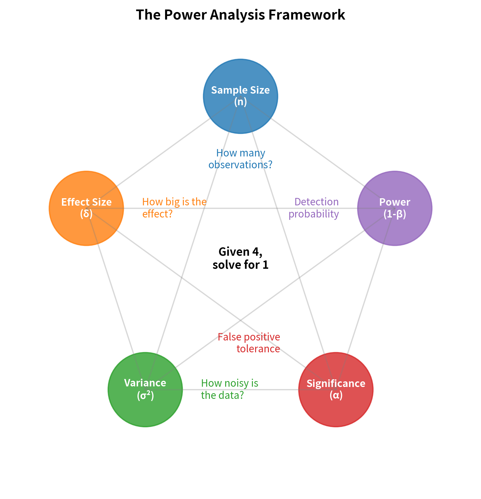
Power analysis connects five interrelated quantities. Given any four, you can solve for the fifth:
The Five Quantities
1. Sample Size (n): The number of observations in your study. Larger samples provide more information and reduce uncertainty.
2. Effect Size (δ): The magnitude of the true effect you're trying to detect. This can be expressed in raw units (e.g., "10 mmHg reduction in blood pressure") or standardized units (e.g., Cohen's d = 0.5).
3. Population Variance (σ²): The natural variability in your measurements. More variance means more noise, making signals harder to detect.
4. Significance Level (α): The probability of Type I error you're willing to accept. Lower α means more stringent requirements for rejecting the null hypothesis.
5. Power (1 - β): The probability of correctly detecting a true effect. Higher power means greater sensitivity to real effects.
The Relationships
These quantities are connected by fundamental relationships that govern all hypothesis tests:
- Larger sample sizes increase power because more data reduces sampling variability
- Larger effect sizes increase power because bigger signals are easier to detect
- Higher variance decreases power because more noise obscures the signal
- Lower α decreases power because stricter criteria make rejection harder
- Targeting higher power requires larger samples to achieve greater sensitivity
Deriving the Sample Size Formula
Let's derive the sample size formula for the most common case: a one-sample z-test. The same logic extends to other tests with minor modifications.
Setup
We want to test:
- (null hypothesis)
- (specific alternative, where )
With:
- Known population standard deviation σ
- Significance level α (two-tailed)
- Desired power 1 - β
The Derivation
Step 1: Find the rejection criterion under H₀
Under the null hypothesis, the test statistic follows N(0, 1).
We reject when , which corresponds to:
Step 2: Calculate power under H₁
Under the alternative , we want:
For a one-sided test (detecting ), the power is:
Under , . Standardizing:
Step 3: Solve for n
Setting power equal to :
This means:
Note: is the z-value such that , so .
Solving for n:
where is the standardized effect size (Cohen's d).
Sample Size Formulas for Common Tests
Different tests require slightly different formulas. Here are the most common ones:
Two-Sample t-test (Equal Variances)
For comparing two independent groups with observations each:
The factor of 2 accounts for the increased variance when comparing two groups.
Paired t-test
For paired observations (before/after, matched pairs):
where and is the standard deviation of the differences.
The paired design is typically more efficient because it removes between-subject variability.
Test for Two Proportions
For comparing two proportions and :
where .
Summary Table
| Test Type | Sample Size Formula | Notes |
|---|---|---|
| One-sample z/t | d = δ/σ | |
| Two-sample t | n per group | |
| Paired t | n pairs, d = δ/σ_d | |
| Two proportions | Complex formula above | n per group |
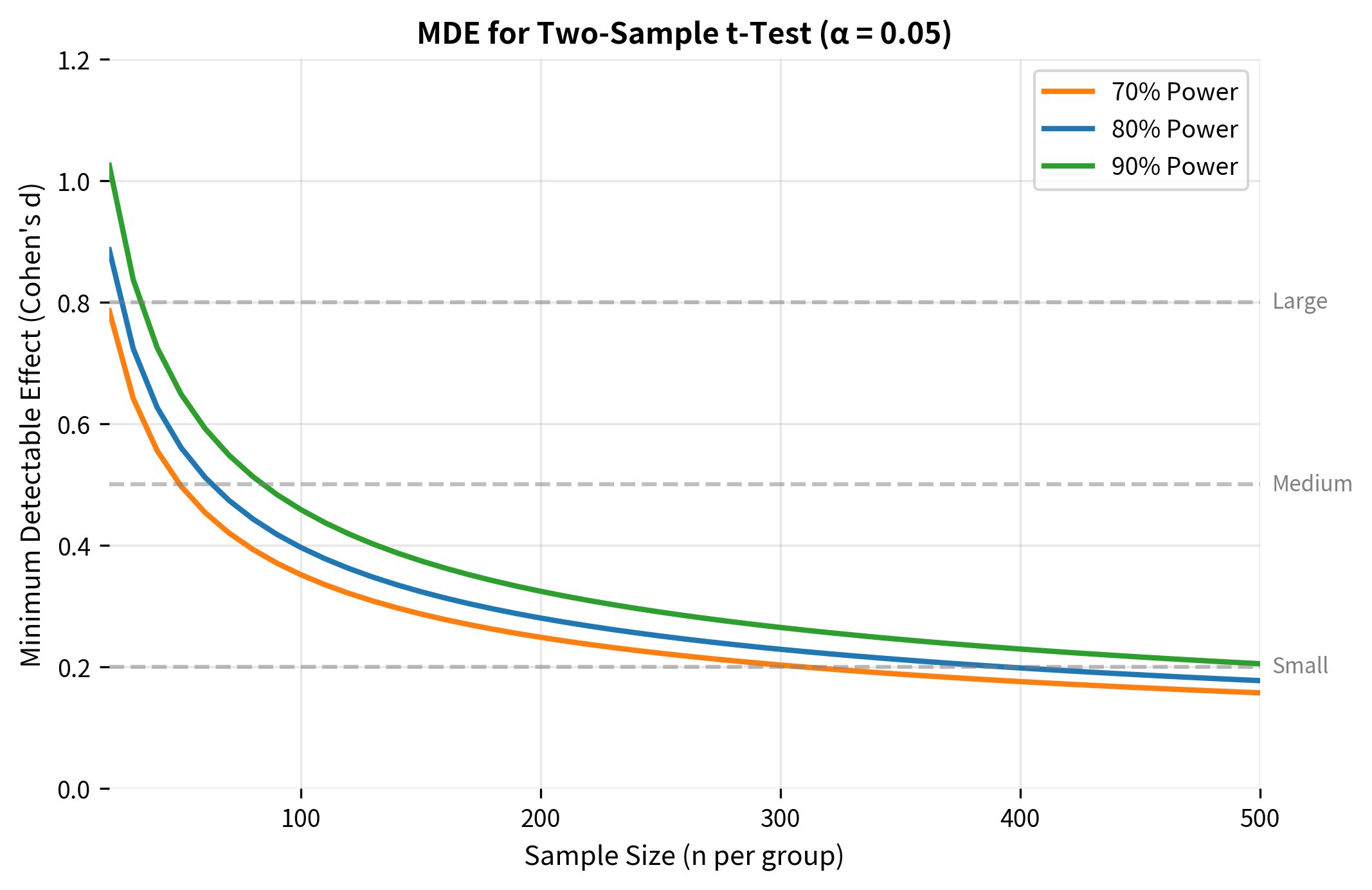
Minimum Detectable Effect (MDE)
Sometimes you have a fixed sample size (due to budget, time, or available participants) and need to know: What's the smallest effect this study can reliably detect?
The minimum detectable effect (MDE) answers this question. It's the effect size threshold below which your study has inadequate power.
Deriving the MDE Formula
Rearranging the sample size formula to solve for effect size:
For a two-sample test:
MDE in Practice: A/B Testing
MDE is particularly important for A/B testing in tech companies. Before running an experiment, you need to know:
- What's the smallest improvement worth detecting?
- How much traffic/time do we need to detect it?
This analysis reveals an important truth: detecting small improvements in conversion rates requires very large samples. A 10% relative lift on a 3% baseline means detecting a 0.3 percentage point improvement, which requires roughly 35,000 users per group.
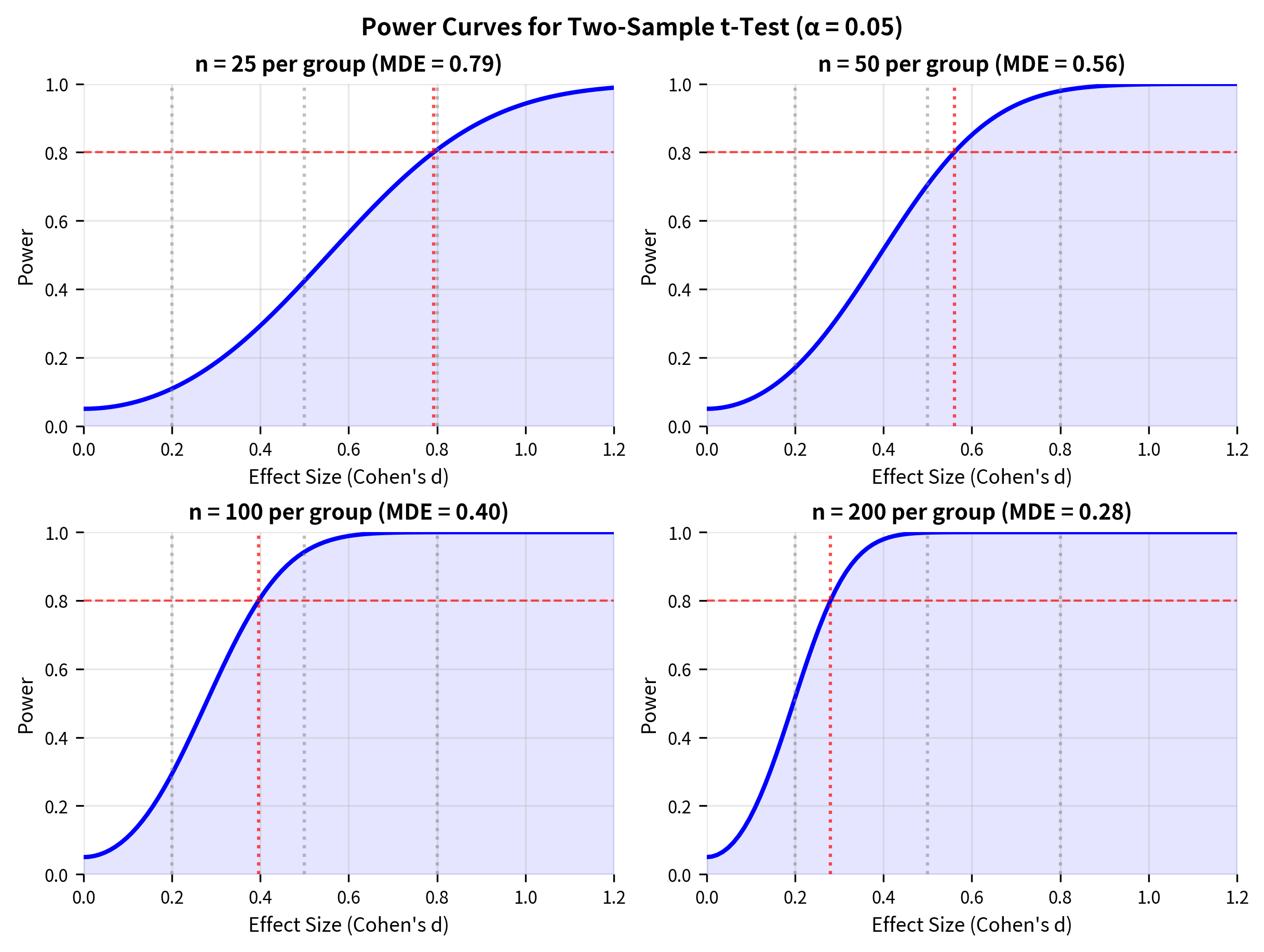
Visualizing Power Analysis
Understanding how the five quantities interact is easier with visualization.

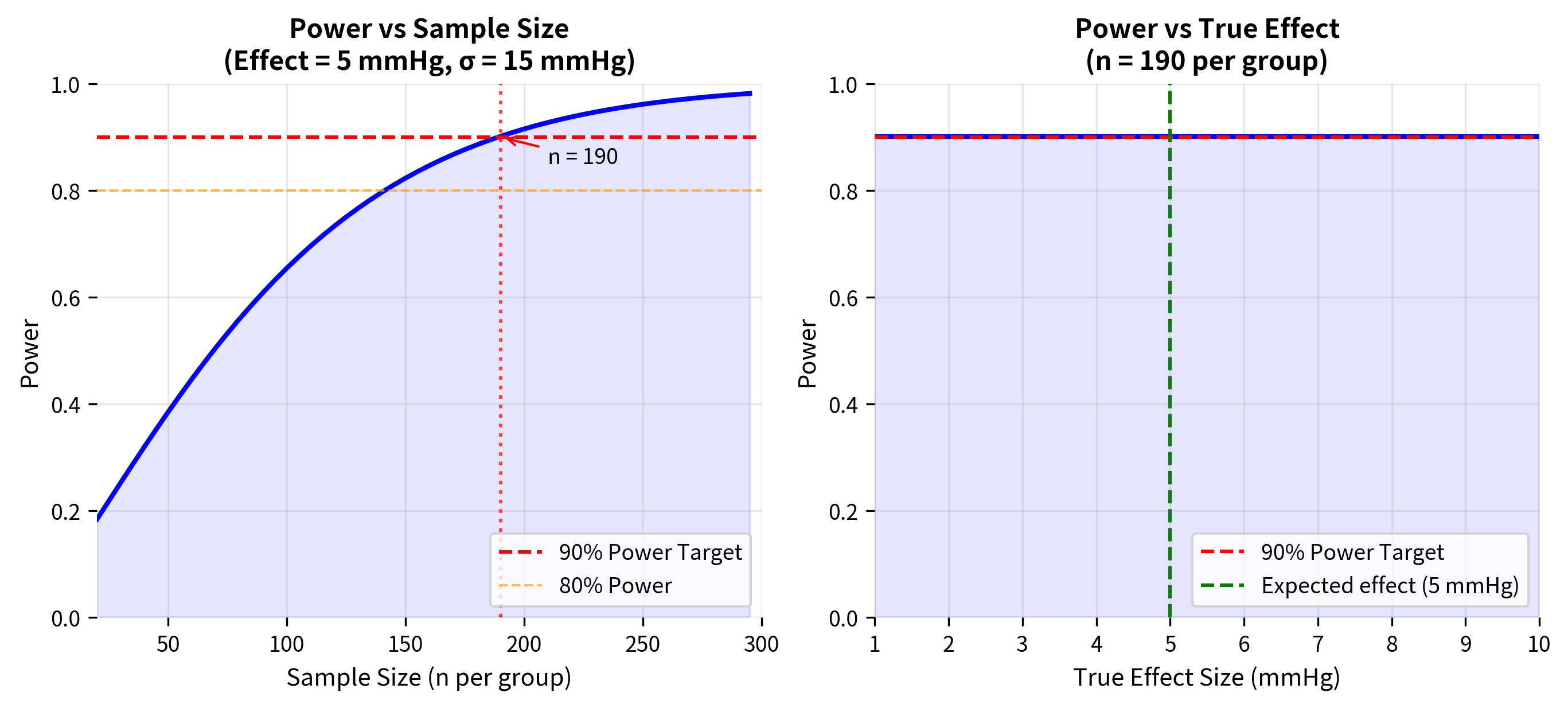
Worked Example: Clinical Trial Design
Let's work through a complete power analysis for a realistic scenario.
Scenario: A pharmaceutical company is designing a clinical trial to test whether a new blood pressure medication reduces systolic blood pressure more than the current standard treatment. Based on pilot data:
- Current treatment reduces systolic BP by 10 mmHg on average
- Standard deviation of BP reduction is approximately 15 mmHg
- The company wants to detect a 5 mmHg additional reduction (clinically meaningful)
- They want 90% power to ensure reliable results
- Using standard α = 0.05 (two-tailed)
Decision Summary
The Problem of Underpowered Studies
Underpowered studies are one of the most pervasive problems in research. When a study has insufficient power:
Consequences of Low Power
1. High False Negative Rate: Real effects are missed because the study lacks sensitivity to detect them. This wastes resources and may lead to abandoning potentially useful treatments or interventions.
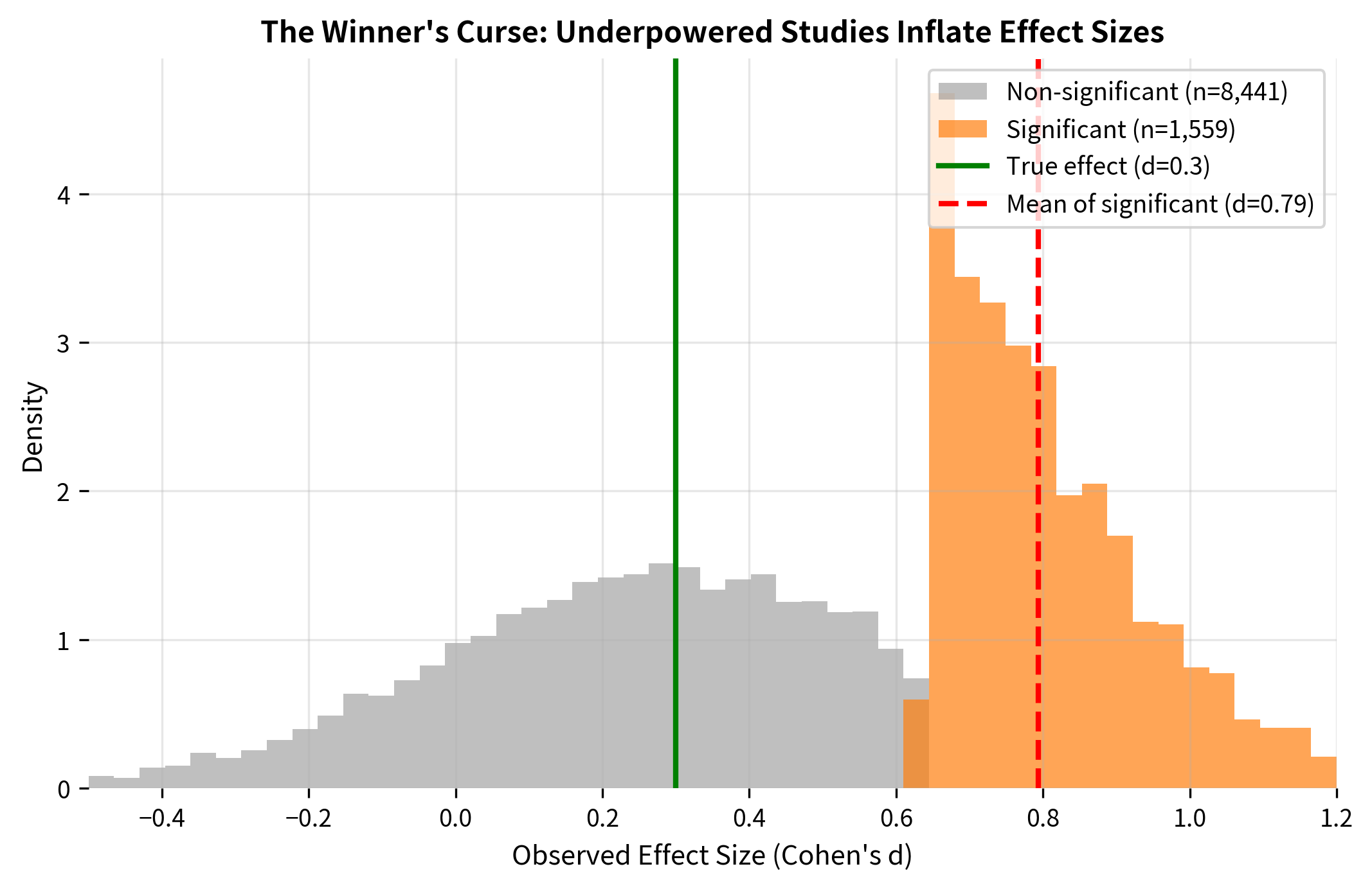
2. Winner's Curse (Effect Size Inflation): When an underpowered study does achieve significance, the estimated effect size is systematically inflated. Only the "lucky" samples with upward random fluctuations cross the significance threshold.
3. Non-Replicability: Inflated effect sizes from underpowered studies are unlikely to replicate. Follow-up studies with the same sample size will often fail to reach significance, contributing to the "replication crisis."
4. Wasted Resources: Underpowered studies waste time, money, and participant effort on research that cannot reliably answer the question being asked.
Avoiding Underpowered Studies
The solution is straightforward: conduct power analysis before data collection. This involves:
-
Specify the smallest effect size of practical importance: What's the minimum effect worth detecting? This is a scientific/business question, not a statistical one.
-
Choose target power: The convention is 80%, but 90% is better for confirmatory research.
-
Calculate required sample size: Use the formulas and tools covered in this section.
-
If required sample is infeasible: Either accept lower power (with documented limitations), seek more funding/participants, or consider whether the study should be conducted at all.
An underpowered study with uncertain results is often worse than no study at all, because it can mislead future research and policy decisions.
Practical Power Analysis Tools
While understanding the formulas is important, in practice you'll often use software tools.
Python: statsmodels
Power Analysis Checklist
When planning a study, work through this checklist:
-
Define the hypothesis clearly: What exactly are you testing?
-
Determine the appropriate test: One-sample, two-sample, paired, proportions, etc.
-
Specify the minimum effect size of interest: Based on practical significance, not statistical convenience.
-
Estimate population variance: From pilot data, literature, or conservative assumptions.
-
Choose significance level: Usually α = 0.05, but consider context.
-
Set target power: At least 80%, preferably 90% for confirmatory research.
-
Calculate required sample size: Using appropriate formulas or software.
-
Conduct sensitivity analysis: What if assumptions are wrong?
-
Document all assumptions: For transparency and reproducibility.
-
Assess feasibility: Is the required sample achievable?
Summary
Power analysis is essential for designing studies that can actually answer research questions. The key points are:
The five quantities (sample size, effect size, variance, α, power) are mathematically connected. Given any four, you can solve for the fifth.
Sample size formulas vary by test type but share a common structure. The key insight is that requirements scale with the square of the ratio (z_α + z_β)/d, so small changes in effect size dramatically affect sample needs.
Minimum detectable effect (MDE) tells you the smallest effect your study can reliably detect. This is crucial for assessing whether a study is worth conducting.
Underpowered studies have serious consequences: high false negative rates, inflated effect estimates (winner's curse), and poor replicability.
Power analysis should be done before data collection, not after. Post-hoc power analysis is meaningless because it's just a transformation of the p-value.
Sensitivity analysis is important because effect size and variance assumptions are often uncertain. Understand how your conclusions change if assumptions are wrong.
What's Next
With sample size determination mastered, you're ready to explore effect sizes in depth. Effect sizes quantify the magnitude of effects in standardized units, making them comparable across studies and contexts. You'll learn:
- Why statistical significance is not the same as practical significance
- How to calculate and interpret various effect size measures
- The relationship between effect size, sample size, and significance
- How to report effect sizes alongside p-values for complete statistical reporting
After effect sizes, you'll learn about multiple comparisons: what happens to power and error rates when you conduct many tests simultaneously. The final section ties all these concepts together with practical guidelines for statistical analysis and reporting.
Quiz
Ready to test your understanding? Take this quick quiz to reinforce what you've learned about sample size, minimum detectable effect, and power analysis.

Comments