Hypothesis Testing Summary & Practical Guide: Reporting, Test Selection & scipy.stats

Michael BrenndoerferJanuary 10, 202618 min read

Practical reporting guidelines, summary of key concepts, test selection parameters table, multiple comparison corrections table, and scipy.stats functions reference. Complete reference guide for hypothesis testing.

Reading Level

Choose your expertise level to adjust how many terms are explained. Beginners see more tooltips, experts see fewer to maintain reading flow. Hover over underlined terms for instant definitions.

Summary and Practical Guide to Hypothesis Testing

In 1925, Ronald Fisher published Statistical Methods for Research Workers, introducing hypothesis testing to the scientific world. His framework revolutionized how we learn from data, providing a rigorous method for distinguishing signal from noise. Nearly a century later, hypothesis testing remains the backbone of empirical research across every scientific discipline: from medicine and psychology to economics and machine learning.

Yet despite its ubiquity, hypothesis testing is frequently misused and misunderstood. Studies show that many published papers contain statistical errors, misinterpret p-values, or fail to report essential information. The goal of this final chapter is to synthesize everything you've learned into a practical guide that helps you avoid these pitfalls and conduct hypothesis tests that are both valid and useful.

This chapter serves as your reference manual: a complete framework for choosing the right test, conducting the analysis correctly, and reporting results in a way that advances scientific knowledge. Keep it handy whenever you're working with data.

The Complete Hypothesis Testing Workflow

Before diving into details, here's the complete workflow for conducting a hypothesis test. Each step is critical: skipping any one can invalidate your conclusions.
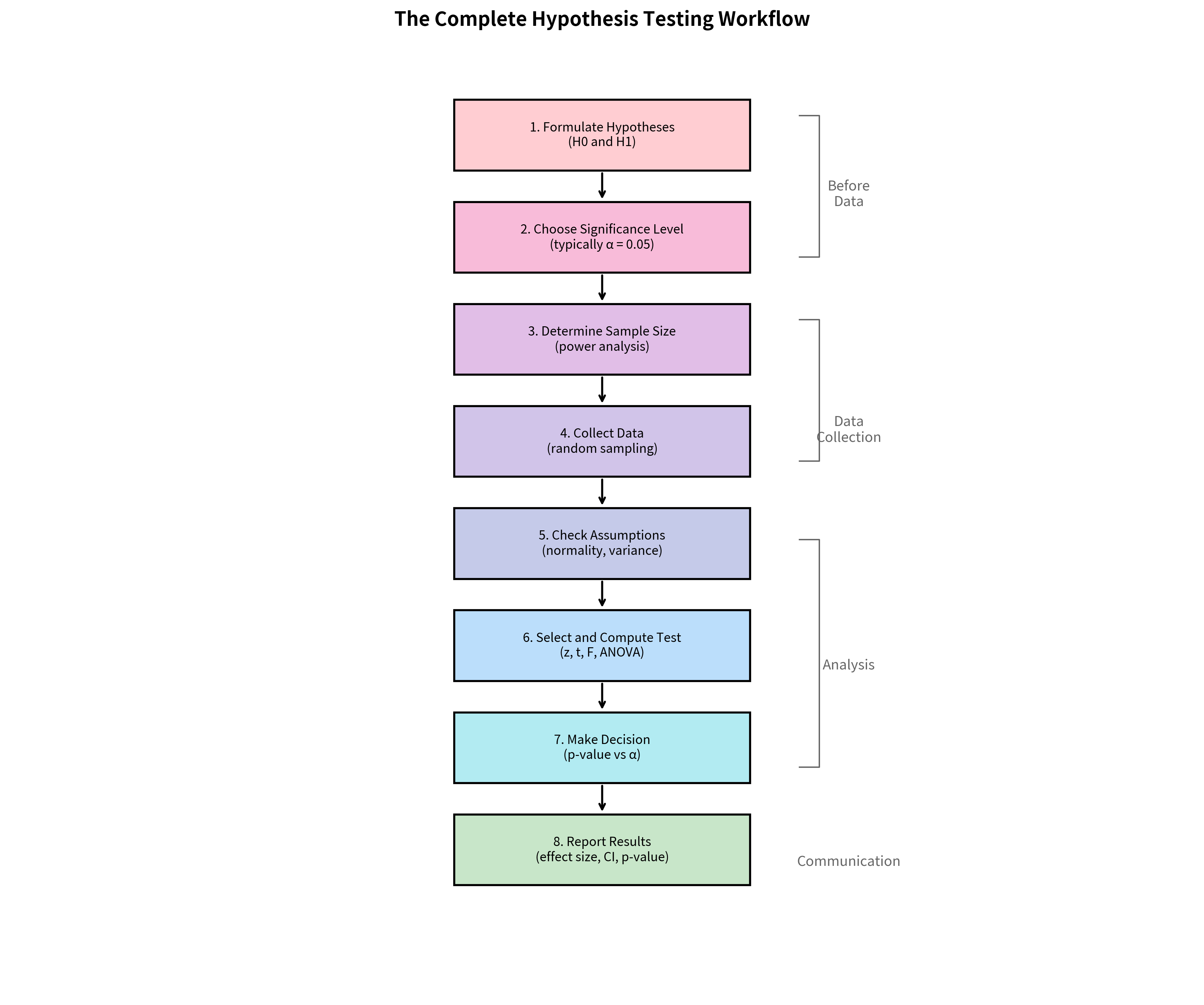
In[3]:
Code
fig, ax = plt.subplots(figsize=(12, 10))
ax.set_xlim(0, 12)
ax.set_ylim(0, 12)
ax.axis("off")


def draw_box(x, y, w, h, text, color, fontsize=9):
    rect = plt.Rectangle(
        (x, y),
        w,
        h,
        facecolor=color,
        edgecolor="black",
        linewidth=1.5,
        zorder=2,
    )
    ax.add_patch(rect)
    ax.text(
        x + w / 2,
        y + h / 2,
        text,
        ha="center",
        va="center",
        fontsize=fontsize,
        wrap=True,
        zorder=3,
    )


def draw_arrow(x1, y1, x2, y2):
    ax.annotate(
        "",
        xy=(x2, y2),
        xytext=(x1, y1),
        arrowprops=dict(arrowstyle="->", color="black", lw=1.5),
        zorder=1,
    )


# Step boxes
steps = [
    (4.5, 10.5, 3, 0.9, "1. Formulate Hypotheses\n(H0 and H1)", "#ffcdd2"),
    (
        4.5,
        9.2,
        3,
        0.9,
        "2. Choose Significance Level\n(typically α = 0.05)",
        "#f8bbd9",
    ),
    (4.5, 7.9, 3, 0.9, "3. Determine Sample Size\n(power analysis)", "#e1bee7"),
    (4.5, 6.6, 3, 0.9, "4. Collect Data\n(random sampling)", "#d1c4e9"),
    (
        4.5,
        5.3,
        3,
        0.9,
        "5. Check Assumptions\n(normality, variance)",
        "#c5cae9",
    ),
    (
        4.5,
        4.0,
        3,
        0.9,
        "6. Select and Compute Test\n(z, t, F, ANOVA)",
        "#bbdefb",
    ),
    (4.5, 2.7, 3, 0.9, "7. Make Decision\n(p-value vs α)", "#b2ebf2"),
    (
        4.5,
        1.4,
        3,
        0.9,
        "8. Report Results\n(effect size, CI, p-value)",
        "#c8e6c9",
    ),
]

for x, y, w, h, text, color in steps:
    draw_box(x, y, w, h, text, color)

# Arrows between steps
for i in range(len(steps) - 1):
    draw_arrow(6, steps[i][1], 6, steps[i + 1][1] + steps[i + 1][3])

# Side annotations
ax.text(
    8.5,
    10.2,
    "Before\nData",
    fontsize=10,
    ha="center",
    va="center",
    style="italic",
    color="#666",
)
ax.text(
    8.5,
    7.2,
    "Data\nCollection",
    fontsize=10,
    ha="center",
    va="center",
    style="italic",
    color="#666",
)
ax.text(
    8.5,
    4.2,
    "Analysis",
    fontsize=10,
    ha="center",
    va="center",
    style="italic",
    color="#666",
)
ax.text(
    8.5,
    1.7,
    "Communication",
    fontsize=10,
    ha="center",
    va="center",
    style="italic",
    color="#666",
)

# Bracket
ax.plot([8, 8.2, 8.2, 8], [11.2, 11.2, 9.4, 9.4], color="#666", lw=1)
ax.plot([8, 8.2, 8.2, 8], [8.6, 8.6, 6.8, 6.8], color="#666", lw=1)
ax.plot([8, 8.2, 8.2, 8], [5.8, 5.8, 2.9, 2.9], color="#666", lw=1)

ax.set_title(
    "The Complete Hypothesis Testing Workflow",
    fontsize=14,
    fontweight="bold",
    y=1.02,
)
plt.show()
Out[3]:
Visualization
Flowchart showing the 8 steps of hypothesis testing from formulating hypotheses to reporting results.
The complete hypothesis testing workflow. Following these steps in order ensures valid and interpretable results. Note that many decisions (hypotheses, α level, sample size) should be made before data collection.

Step-by-Step Guide

Step 1: Formulate Hypotheses

  • Define H0H_0 (null hypothesis): The default assumption, typically "no effect" or "no difference"
  • Define H1H_1 (alternative hypothesis): What you're trying to demonstrate
  • Choose one-tailed or two-tailed based on your research question
  • Do this BEFORE seeing the data

Step 2: Choose Significance Level (α)

  • Standard: α = 0.05 (5% false positive rate)
  • Stringent: α = 0.01 for high-stakes decisions
  • Lenient: α = 0.10 for exploratory research
  • Consider the consequences of Type I vs Type II errors

Step 3: Determine Sample Size

  • Use power analysis to calculate required n
  • Specify: α, power (typically 0.80), minimum effect size of interest
  • Balance statistical needs against practical constraints

Step 4: Collect Data

  • Use appropriate randomization and sampling methods
  • Ensure independence of observations
  • Avoid peeking at results during collection

Step 5: Check Assumptions

  • Normality: Shapiro-Wilk test, Q-Q plots
  • Equal variances: Levene's test
  • Independence: Study design consideration
  • Choose robust alternatives if assumptions violated

Step 6: Select and Compute Test

Step 7: Make Decision

  • If p < α: Reject H₀, conclude evidence for H₁
  • If p ≥ α: Fail to reject H₀, insufficient evidence
  • Remember: "fail to reject" ≠ "accept H₀"

Step 8: Report Results

  • Effect size (Cohen's d, η², r)
  • Confidence interval
  • Exact p-value
  • Test statistic and degrees of freedom
  • Assumption check results

Test Selection Decision Tree

Choosing the correct test is critical. Use this decision framework based on your research question and data characteristics.

Out[4]:
Visualization
Decision tree diagram for selecting hypothesis tests based on data type and research question.
Decision tree for selecting the appropriate hypothesis test. Start at the top and follow the branches based on your research question and data structure.

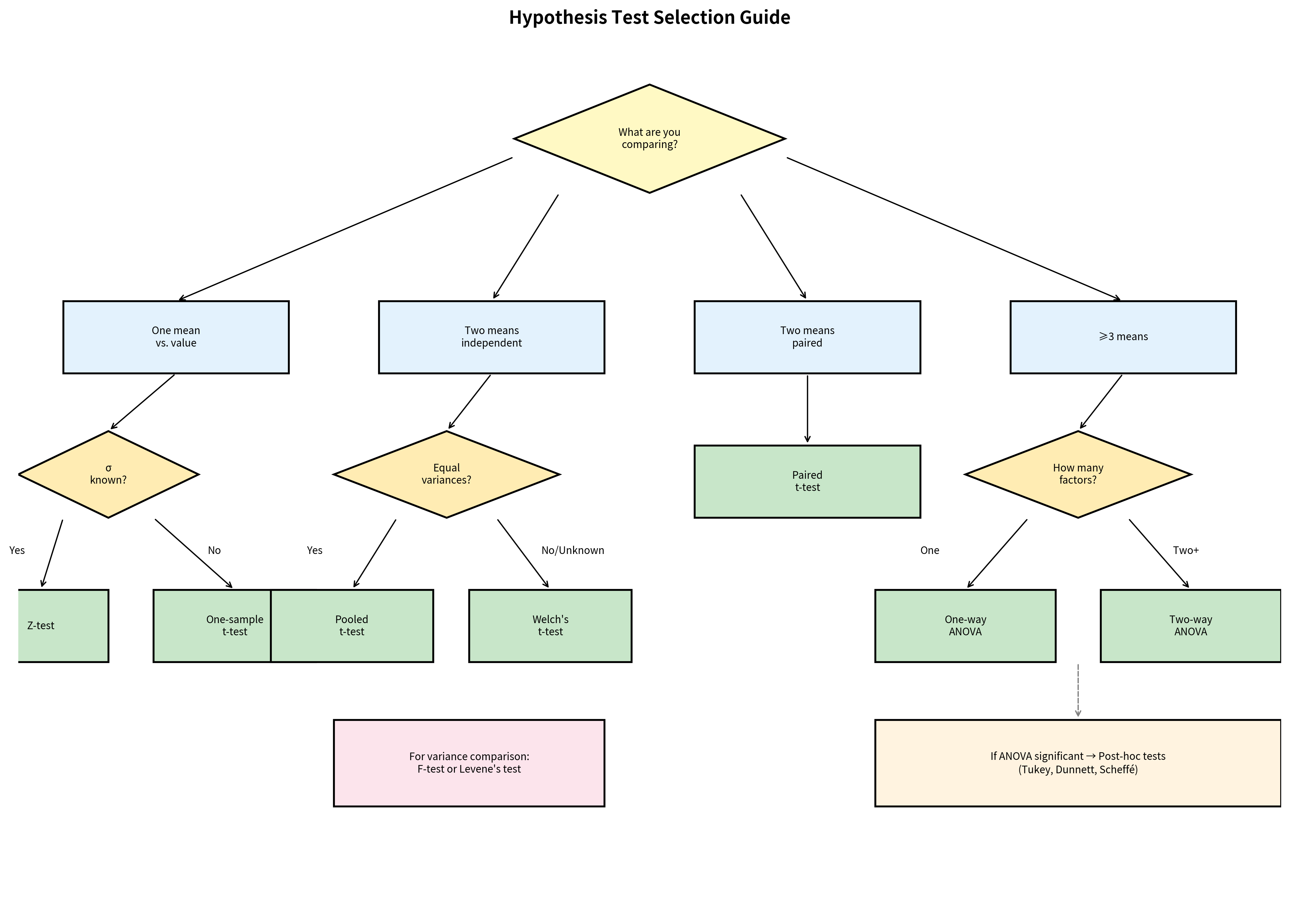
Quick Reference Table

Research QuestionTestscipy.stats Function
Is the mean equal to a specific value? (σ known)Z-testManual calculation
Is the mean equal to a specific value? (σ unknown)One-sample t-testttest_1samp()
Are two independent group means equal?Welch's t-testttest_ind(equal_var=False)
Are two independent group means equal? (equal var)Pooled t-testttest_ind(equal_var=True)
Are paired/matched observations different?Paired t-testttest_rel()
Are ≥3 group means equal?One-way ANOVAf_oneway()
Are two variances equal?F-testf.sf() (manual)
Are multiple variances equal?Levene's testlevene()
Which pairs differ after ANOVA?Tukey HSDtukey_hsd()
Treatment vs control comparisons?Dunnett's testdunnett()

Effect Size Reference

Effect sizes quantify the magnitude of an effect independent of sample size. Always report them alongside p-values.

Cohen's d (Comparing Two Means)

d=xˉ1xˉ2spooledd = \frac{\bar{x}_1 - \bar{x}_2}{s_{\text{pooled}}}

Cohen's dInterpretationPractical Example
0.2SmallSubtle difference, requires large sample to detect
0.5MediumNoticeable effect, visible with moderate sample
0.8LargeSubstantial effect, obvious in most analyses
1.2+Very largeMajor effect, visible to naked eye

Related measures:

  • Hedges' g: Corrects d for small sample bias
  • Glass's Δ: Uses control group SD only
  • Cohen's d_z: For paired designs, uses SD of differences

ANOVA Effect Sizes

MeasureFormulaInterpretation
η² (eta-squared)SSbetween/SStotalSS_{\text{between}} / SS_{\text{total}}% variance explained (biased upward)
ω² (omega-squared)Corrected formulaLess biased estimate
Partial η²For factorial designsEffect controlling for other factors

Benchmarks for η² and ω²:

  • Small: 0.01
  • Medium: 0.06
  • Large: 0.14

Correlation as Effect Size

rInterpretationr² (variance explained)
0.1Small1%
0.3Medium9%
0.5Large25%

Power Analysis Quick Reference

Power analysis determines the sample size needed to detect an effect of a given size with specified probability.

The Power Pentagon

Five quantities are interconnected: knowing any four determines the fifth:

  1. Sample size (n): Number of observations
  2. Effect size (d): Magnitude of the effect
  3. Significance level (α): False positive rate
  4. Power (1-β): True positive rate
  5. Variability (σ): Data spread

Sample Size Formulas

One-sample t-test: n=(z1α/2+z1βd)2n = \left(\frac{z_{1-\alpha/2} + z_{1-\beta}}{d}\right)^2

Two-sample t-test (equal groups): nper group=2(z1α/2+z1βd)2n_{\text{per group}} = 2\left(\frac{z_{1-\alpha/2} + z_{1-\beta}}{d}\right)^2

Two proportions: nper group=2pˉ(1pˉ)(z1α/2+z1β)2(p1p2)2n_{\text{per group}} = \frac{2\bar{p}(1-\bar{p})(z_{1-\alpha/2} + z_{1-\beta})^2}{(p_1 - p_2)^2}

Sample Size Table (Two-Sample t-test, α = 0.05, Two-tailed)

Effect SizePower = 0.80Power = 0.90Power = 0.95
d = 0.2 (small)394 per group527 per group651 per group
d = 0.5 (medium)64 per group86 per group105 per group
d = 0.8 (large)26 per group34 per group42 per group
In[5]:
Code
# Power analysis with statsmodels
from statsmodels.stats.power import TTestIndPower

analysis = TTestIndPower()

# Calculate required sample size
n = analysis.solve_power(effect_size=0.5, power=0.8, alpha=0.05)
print(f"For d=0.5, power=0.80, α=0.05: n = {n:.0f} per group")

# Calculate power for given sample size
power = analysis.solve_power(effect_size=0.5, nobs1=50, alpha=0.05)
print(f"For d=0.5, n=50/group, α=0.05: power = {power:.2f}")

# Calculate detectable effect size
mde = analysis.solve_power(nobs1=100, power=0.8, alpha=0.05)
print(f"For n=100/group, power=0.80, α=0.05: MDE = {mde:.3f}")
Out[5]:
Console
For d=0.5, power=0.80, α=0.05: n = 64 per group
For d=0.5, n=50/group, α=0.05: power = 0.70
For n=100/group, power=0.80, α=0.05: MDE = 0.398

Multiple Comparisons Reference

When to Use Each Method

MethodControlsUse When
BonferroniFWERFew tests, any false positive costly
HolmFWERMany tests, need more power than Bonferroni
Benjamini-HochbergFDRExploratory analysis, many tests OK
Tukey HSDFWERAll pairwise comparisons after ANOVA
DunnettFWERComparing treatments to control

Quick Formulas

Bonferroni: Reject if pi<α/mp_i < \alpha/m

Holm (step-down): For ordered p-values, reject p(j)p_{(j)} if p(j)<α/(mj+1)p_{(j)} < \alpha/(m-j+1)

Benjamini-Hochberg: Find largest kk where p(k)kmqp_{(k)} \leq \frac{k}{m}q, reject all pp(k)p \leq p_{(k)}

In[6]:
Code
from scipy.stats import false_discovery_control

# Example: 5 p-values from multiple tests
p_values = [0.001, 0.008, 0.039, 0.041, 0.23]

# Bonferroni
bonf_threshold = 0.05 / len(p_values)
bonf_reject = [p < bonf_threshold for p in p_values]
print(f"Bonferroni (threshold = {bonf_threshold:.3f}): {bonf_reject}")

# Benjamini-Hochberg
bh_adjusted = false_discovery_control(p_values, method="bh")
bh_reject = bh_adjusted < 0.05
print(f"BH adjusted p-values: {[f'{p:.3f}' for p in bh_adjusted]}")
print(f"BH reject: {list(bh_reject)}")
Out[6]:
Console
Bonferroni (threshold = 0.010): [True, True, False, False, False]
BH adjusted p-values: ['0.005', '0.020', '0.051', '0.051', '0.230']
BH reject: [np.True_, np.True_, np.False_, np.False_, np.False_]

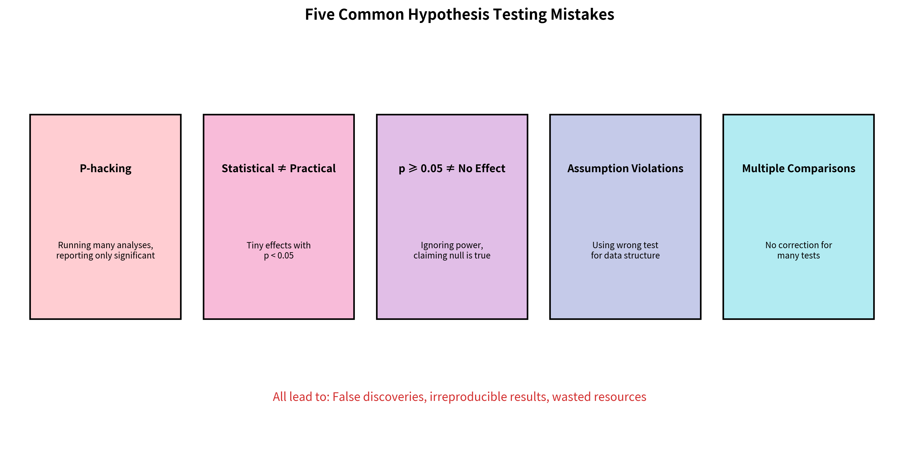
Common Mistakes and How to Avoid Them

Mistake 1: P-Hacking

Problem: Running multiple analyses and only reporting significant results.

Solution: Pre-register your analysis plan. Report all tests conducted, not just significant ones. Use appropriate multiple comparison corrections.

Mistake 2: Confusing Statistical and Practical Significance

Problem: Treating p < 0.05 as proof that an effect matters.

Solution: Always report effect sizes. Ask "Is this effect large enough to be meaningful?" even when statistically significant.

Mistake 3: Misinterpreting Non-Significant Results

Problem: Concluding "no effect exists" when p ≥ 0.05.

Solution: Consider statistical power. Report confidence intervals to show the range of plausible effects. Distinguish "evidence of absence" from "absence of evidence."

Mistake 4: Violating Assumptions

Problem: Using parametric tests when assumptions are violated.

Solution: Check assumptions before testing. Use robust alternatives (Welch's t-test, non-parametric tests) when assumptions fail.

Mistake 5: Ignoring Multiple Comparisons

Problem: Running many tests without correction, inflating false positive rate.

Solution: Plan your analyses in advance. Apply appropriate corrections. Report the number of tests conducted.

In[7]:
Code
fig, ax = plt.subplots(figsize=(12, 6))
ax.set_xlim(0, 12)
ax.set_ylim(0, 6)
ax.axis("off")

mistakes = [
    (
        "P-hacking",
        "Running many analyses,\nreporting only significant",
        "#ffcdd2",
    ),
    ("Statistical ≠ Practical", "Tiny effects with\np < 0.05", "#f8bbd9"),
    (
        "p ≥ 0.05 ≠ No Effect",
        "Ignoring power,\nclaiming null is true",
        "#e1bee7",
    ),
    (
        "Assumption Violations",
        "Using wrong test\nfor data structure",
        "#c5cae9",
    ),
    ("Multiple Comparisons", "No correction for\nmany tests", "#b2ebf2"),
]

for i, (title, desc, color) in enumerate(mistakes):
    x = 0.3 + i * 2.3
    rect = plt.Rectangle(
        (x, 2), 2, 3, facecolor=color, edgecolor="black", linewidth=1.5
    )
    ax.add_patch(rect)
    ax.text(
        x + 1,
        4.2,
        title,
        ha="center",
        va="center",
        fontsize=10,
        fontweight="bold",
    )
    ax.text(x + 1, 3, desc, ha="center", va="center", fontsize=8)

ax.text(
    6,
    0.8,
    "All lead to: False discoveries, irreproducible results, wasted resources",
    ha="center",
    fontsize=11,
    style="italic",
    color="#d32f2f",
)

ax.set_title(
    "Five Common Hypothesis Testing Mistakes",
    fontsize=14,
    fontweight="bold",
    y=1.05,
)
plt.show()
Out[7]:
Visualization
Diagram showing common hypothesis testing mistakes with visual indicators of their severity.
The five most common hypothesis testing mistakes and their consequences. Each error can lead to misleading conclusions and irreproducible results.

Complete Reporting Example

Here's an example of a complete analysis with proper reporting:

In[8]:
Code
import numpy as np
from scipy import stats

# Research question: Does a new teaching method improve test scores?
np.random.seed(42)
control = np.random.normal(75, 12, 30)  # Traditional method
treatment = np.random.normal(82, 11, 30)  # New method

# 1. Descriptive statistics
print("=" * 60)
print("DESCRIPTIVE STATISTICS")
print("=" * 60)
print(
    f"Control:   n = {len(control)}, M = {np.mean(control):.2f}, SD = {np.std(control, ddof=1):.2f}"
)
print(
    f"Treatment: n = {len(treatment)}, M = {np.mean(treatment):.2f}, SD = {np.std(treatment, ddof=1):.2f}"
)
print()

# 2. Check assumptions
print("=" * 60)
print("ASSUMPTION CHECKS")
print("=" * 60)

# Normality
_, p_norm_ctrl = stats.shapiro(control)
_, p_norm_treat = stats.shapiro(treatment)
print(
    f"Shapiro-Wilk (Control):   W = {stats.shapiro(control)[0]:.3f}, p = {p_norm_ctrl:.3f}"
)
print(
    f"Shapiro-Wilk (Treatment): W = {stats.shapiro(treatment)[0]:.3f}, p = {p_norm_treat:.3f}"
)
print("  → Normality assumption supported (p > 0.05 for both groups)")
print()

# Equal variances
_, p_levene = stats.levene(control, treatment)
print(
    f"Levene's test: F = {stats.levene(control, treatment)[0]:.3f}, p = {p_levene:.3f}"
)
print("  → Equal variances assumption supported (p > 0.05)")
print()

# 3. Conduct test
print("=" * 60)
print("HYPOTHESIS TEST")
print("=" * 60)
t_stat, p_value = stats.ttest_ind(treatment, control, equal_var=True)
df = len(control) + len(treatment) - 2
print(f"Two-sample t-test: t({df}) = {t_stat:.3f}, p = {p_value:.4f}")
print()

# 4. Effect size
mean_diff = np.mean(treatment) - np.mean(control)
pooled_std = np.sqrt(
    (
        (len(control) - 1) * np.var(control, ddof=1)
        + (len(treatment) - 1) * np.var(treatment, ddof=1)
    )
    / (len(control) + len(treatment) - 2)
)
cohens_d = mean_diff / pooled_std
print("=" * 60)
print("EFFECT SIZE")
print("=" * 60)
print(f"Mean difference: {mean_diff:.2f} points")
print(f"Cohen's d = {cohens_d:.3f} (large effect)")
print()

# 5. Confidence interval for difference
se_diff = pooled_std * np.sqrt(1 / len(control) + 1 / len(treatment))
t_crit = stats.t.ppf(0.975, df)
ci_lower = mean_diff - t_crit * se_diff
ci_upper = mean_diff + t_crit * se_diff
print("=" * 60)
print("CONFIDENCE INTERVAL")
print("=" * 60)
print(f"95% CI for difference: [{ci_lower:.2f}, {ci_upper:.2f}]")
print()

# 6. Complete report
print("=" * 60)
print("COMPLETE REPORT (APA STYLE)")
print("=" * 60)
print(
    f"Students in the new teaching method condition (M = {np.mean(treatment):.1f}, "
)
print(
    f"SD = {np.std(treatment, ddof=1):.1f}) scored significantly higher than those in the "
)
print(
    f"traditional method condition (M = {np.mean(control):.1f}, SD = {np.std(control, ddof=1):.1f}), "
)
print(
    f"t({df}) = {t_stat:.2f}, p {'< 0.001' if p_value < 0.001 else f'= {p_value:.3f}'}, "
)
print(f"95% CI [{ci_lower:.1f}, {ci_upper:.1f}], Cohen's d = {cohens_d:.2f}.")
Out[8]:
Console
============================================================
DESCRIPTIVE STATISTICS
============================================================
Control:   n = 30, M = 72.74, SD = 10.80
Treatment: n = 30, M = 80.67, SD = 10.24

============================================================
ASSUMPTION CHECKS
============================================================
Shapiro-Wilk (Control):   W = 0.975, p = 0.687
Shapiro-Wilk (Treatment): W = 0.984, p = 0.913
  → Normality assumption supported (p > 0.05 for both groups)

Levene's test: F = 0.002, p = 0.963
  → Equal variances assumption supported (p > 0.05)

============================================================
HYPOTHESIS TEST
============================================================
Two-sample t-test: t(58) = 2.916, p = 0.0050

============================================================
EFFECT SIZE
============================================================
Mean difference: 7.92 points
Cohen's d = 0.753 (large effect)

============================================================
CONFIDENCE INTERVAL
============================================================
95% CI for difference: [2.49, 13.36]

============================================================
COMPLETE REPORT (APA STYLE)
============================================================
Students in the new teaching method condition (M = 80.7, 
SD = 10.2) scored significantly higher than those in the 
traditional method condition (M = 72.7, SD = 10.8), 
t(58) = 2.92, p = 0.005, 
95% CI [2.5, 13.4], Cohen's d = 0.75.

scipy.stats Quick Reference

Testing Functions

In[17]:
Code
from scipy import stats

# One-sample tests
stats.ttest_1samp(sample, popmean)  # One-sample t-test
stats.shapiro(sample)  # Normality test

# Two-sample tests
stats.ttest_ind(a, b, equal_var=True)  # Pooled t-test
stats.ttest_ind(a, b, equal_var=False)  # Welch's t-test
stats.ttest_rel(a, b)  # Paired t-test
stats.levene(a, b)  # Equal variance test

# Multiple groups
stats.f_oneway(g1, g2, g3, ...)  # One-way ANOVA
stats.tukey_hsd(g1, g2, g3, ...)  # Tukey post-hoc
stats.dunnett(t1, t2, control=ctrl)  # Dunnett post-hoc

# Multiple comparison corrections
stats.false_discovery_control(pvals, method="bh")  # BH correction
stats.false_discovery_control(pvals, method="by")  # BY correction

Distribution Functions

In[19]:
Code
# For manual calculations
stats.norm.ppf(0.975)  # Z critical value (two-tailed, α=0.05)
stats.t.ppf(0.975, df)  # t critical value
stats.f.ppf(0.95, df1, df2)  # F critical value

# P-values from test statistics
stats.norm.sf(z) * 2  # Two-tailed p from z
stats.t.sf(t, df) * 2  # Two-tailed p from t
stats.f.sf(f, df1, df2)  # Upper-tail p from F

Summary: Key Takeaways

The Foundations

  1. P-values measure evidence against H₀, not the probability H₀ is true
  2. Confidence intervals show the range of plausible parameter values
  3. Effect sizes quantify magnitude independent of sample size
  4. Power determines your ability to detect effects that exist

The Tests

  1. Z-test: When σ is known (rare in practice)
  2. t-test: The workhorse for comparing means
  3. Welch's t-test: Default for two-group comparisons
  4. ANOVA: For comparing ≥3 groups
  5. Post-hoc tests: After significant ANOVA

The Errors

  1. Type I (α): False positive: rejecting true H₀
  2. Type II (β): False negative: failing to reject false H₀
  3. Multiple comparisons: Inflate error rates without correction

The Practice

  1. Plan before collecting data: Hypotheses, α, sample size
  2. Check assumptions: Normality, equal variances, independence
  3. Report completely: Effect size, CI, exact p-value, test used
  4. Interpret cautiously: Statistical ≠ practical significance

Conclusion

Hypothesis testing is a powerful framework for learning from data, but its power comes with responsibility. The methods you've learned in this series, from basic p-values and confidence intervals to power analysis, effect sizes, and multiple comparison corrections, form a complete toolkit for rigorous statistical inference.

Remember these principles:

  1. Design before analysis: Plan your hypotheses, tests, and sample size before seeing data
  2. Check your assumptions: Use appropriate tests for your data structure
  3. Report completely: Enable others to evaluate and replicate your work
  4. Think beyond p-values: Effect sizes and confidence intervals tell a richer story
  5. Control multiplicity: Correct for multiple tests when applicable

Statistics is not about proving things with certainty: it's about quantifying uncertainty and making informed decisions despite incomplete information. Used well, hypothesis testing helps us separate signal from noise and build cumulative scientific knowledge. Used poorly, it generates false discoveries and wastes resources.

The difference between the two lies in understanding not just how to calculate test statistics, but why each step matters and what can go wrong. With the knowledge from this series, you're equipped to conduct hypothesis tests that are valid, interpretable, and useful.


This concludes the hypothesis testing series. For hands-on practice, try applying these methods to your own data, starting with clear hypotheses and working through each step of the workflow.

Quiz

Ready to test your understanding? Take this comprehensive quiz to reinforce what you've learned throughout the hypothesis testing series.

Loading component...

Reference

BIBTEXAcademic
@misc{hypothesistestingsummarypracticalguidereportingtestselectionscipystats, author = {Michael Brenndoerfer}, title = {Hypothesis Testing Summary & Practical Guide: Reporting, Test Selection & scipy.stats}, year = {2026}, url = {https://mbrenndoerfer.com/writing/hypothesis-testing-summary-practical-guide-reporting-test-selection-scipy-stats}, organization = {mbrenndoerfer.com}, note = {Accessed: 2025-01-01} }
APAAcademic
Michael Brenndoerfer (2026). Hypothesis Testing Summary & Practical Guide: Reporting, Test Selection & scipy.stats. Retrieved from https://mbrenndoerfer.com/writing/hypothesis-testing-summary-practical-guide-reporting-test-selection-scipy-stats
MLAAcademic
Michael Brenndoerfer. "Hypothesis Testing Summary & Practical Guide: Reporting, Test Selection & scipy.stats." 2026. Web. today. <https://mbrenndoerfer.com/writing/hypothesis-testing-summary-practical-guide-reporting-test-selection-scipy-stats>.
CHICAGOAcademic
Michael Brenndoerfer. "Hypothesis Testing Summary & Practical Guide: Reporting, Test Selection & scipy.stats." Accessed today. https://mbrenndoerfer.com/writing/hypothesis-testing-summary-practical-guide-reporting-test-selection-scipy-stats.
HARVARDAcademic
Michael Brenndoerfer (2026) 'Hypothesis Testing Summary & Practical Guide: Reporting, Test Selection & scipy.stats'. Available at: https://mbrenndoerfer.com/writing/hypothesis-testing-summary-practical-guide-reporting-test-selection-scipy-stats (Accessed: today).
SimpleBasic
Michael Brenndoerfer (2026). Hypothesis Testing Summary & Practical Guide: Reporting, Test Selection & scipy.stats. https://mbrenndoerfer.com/writing/hypothesis-testing-summary-practical-guide-reporting-test-selection-scipy-stats