

Family-wise error rate, false discovery rate, Bonferroni correction, Holm's method, and Benjamini-Hochberg procedure. Learn how to control error rates when conducting multiple hypothesis tests.

This article is part of the free-to-read Machine Learning from Scratch
Choose your expertise level to adjust how many terms are explained. Beginners see more tooltips, experts see fewer to maintain reading flow. Hover over underlined terms for instant definitions.
Multiple Comparisons and False Discovery Control
In 2011, neuroscientist Craig Bennett presented a poster at a conference that would become one of the most discussed studies in modern science. He had placed a subject in an fMRI scanner, shown them photographs of people in social situations, and asked them to determine what emotion the person was experiencing. The scanner detected statistically significant brain activity during this task. The catch? The subject was a dead Atlantic salmon.
How could a dead fish show "brain activity"? The answer lies in the multiple comparisons problem. An fMRI scan divides the brain into roughly 130,000 tiny regions called voxels. At each voxel, researchers test whether activity differs from baseline. With 130,000 tests at , we expect about 6,500 false positives purely by chance, more than enough to create apparent "activation patterns" in a dead fish. Bennett's study was a brilliant demonstration of why multiple comparison corrections are essential in modern research.
This chapter explores the mathematics of multiple testing: why conducting many tests inflates error rates, how to quantify this inflation, and the correction methods that restore valid inference. Understanding these concepts is crucial for anyone working with data that involves multiple statistical tests: from genomics and neuroimaging to A/B testing and clinical trials.
The Multiple Comparisons Problem
When we conduct a single hypothesis test at significance level , we accept a 5% chance of a Type I error: rejecting a true null hypothesis. This seems like an acceptable risk. But what happens when we conduct many tests?
The Mathematics of Multiplicity
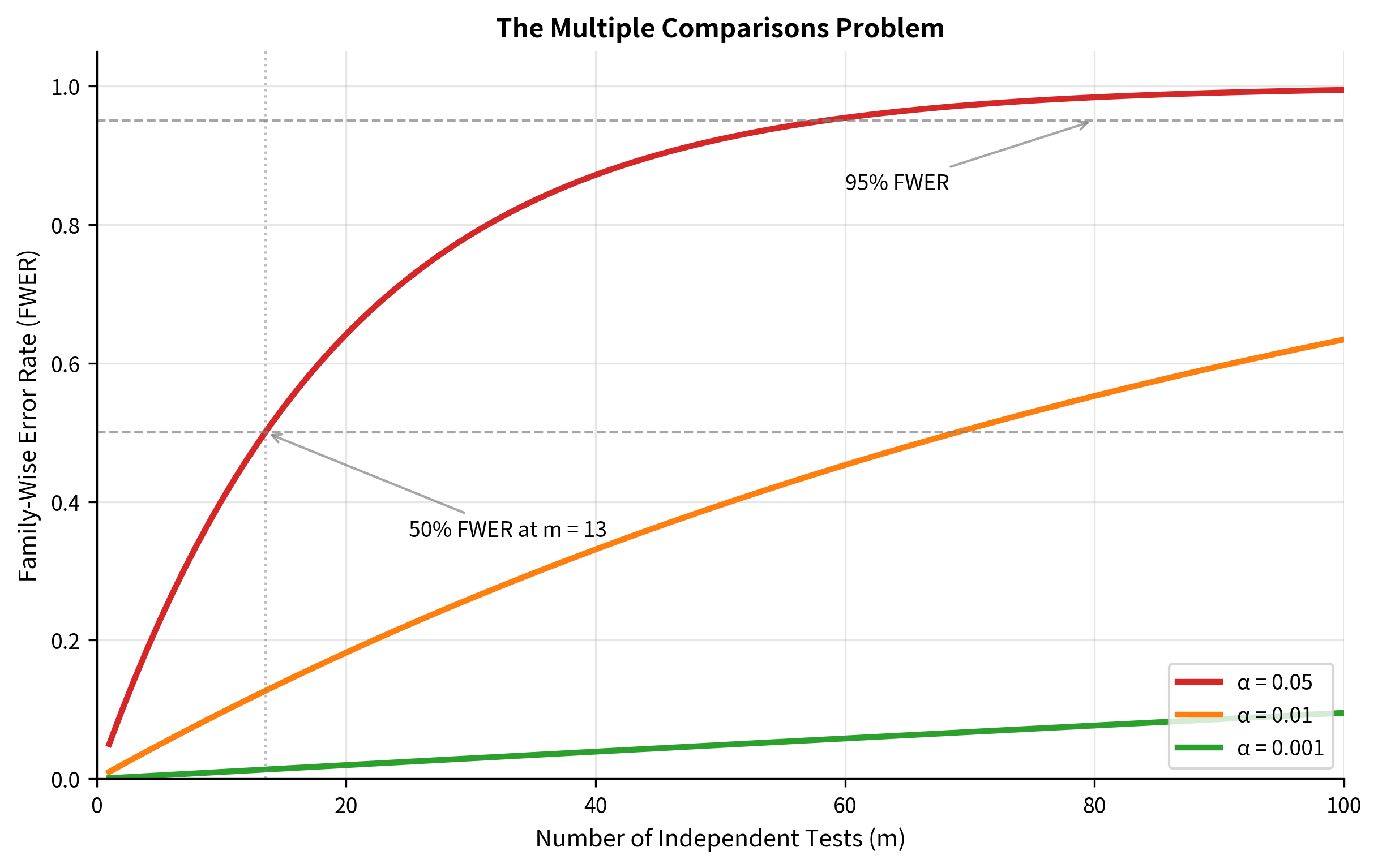
Consider conducting independent hypothesis tests, each at significance level . If all null hypotheses are true, each test has probability of producing a false positive. The probability of making at least one false positive across all tests is:
Since the tests are independent:
Therefore:
This is called the family-wise error rate (FWER): the probability of making at least one Type I error among a family of tests.
Let's see how quickly this grows:
| Number of tests () | FWER at |
|---|---|
| 1 | 0.050 |
| 5 | 0.226 |
| 10 | 0.401 |
| 14 | 0.512 |
| 20 | 0.642 |
| 50 | 0.923 |
| 100 | 0.994 |
With just 14 tests, you have more than a 50% chance of at least one false positive. By 100 tests, a false positive is virtually certain (99.4%).
Simulation: Seeing False Positives Emerge
Let's simulate the multiple comparisons problem directly. We'll generate data where all null hypotheses are true (no real effects) and watch how false positives accumulate.

The simulation confirms our mathematical analysis: with 100 tests and no real effects, we obtained {python} sum(significant) "significant" results, false positives that could mislead researchers into believing they've found real effects.
Error Rate Concepts: FWER vs FDR
Before diving into correction methods, we need to clearly distinguish two different ways to conceptualize error rates in multiple testing. Each has its place depending on your research goals.
Family-Wise Error Rate (FWER)
The family-wise error rate is the probability of making at least one Type I error among all tests:
where is the number of false positives (true null hypotheses incorrectly rejected).
When to control FWER:
- Confirmatory research where conclusions must be definitive
- Clinical trials where each significant result leads to treatment decisions
- Any situation where a single false positive has serious consequences
- Small numbers of pre-specified comparisons
Controlling FWER at level guarantees that the probability of any false positive is at most . This is the most conservative form of error control.
False Discovery Rate (FDR)
The false discovery rate is the expected proportion of false positives among rejected hypotheses:
where is the number of false positives and is the total number of rejections.
When to control FDR:
- Exploratory research where you're screening many hypotheses
- Genomics, proteomics, and other -omics studies
- Neuroimaging with thousands of voxels
- A/B testing with many metrics
- Situations where some false positives are acceptable if most discoveries are real
Controlling FDR at level means that among your "significant" results, the expected proportion of false discoveries is at most . This allows more discoveries while still controlling the error rate.
Visualizing the Difference
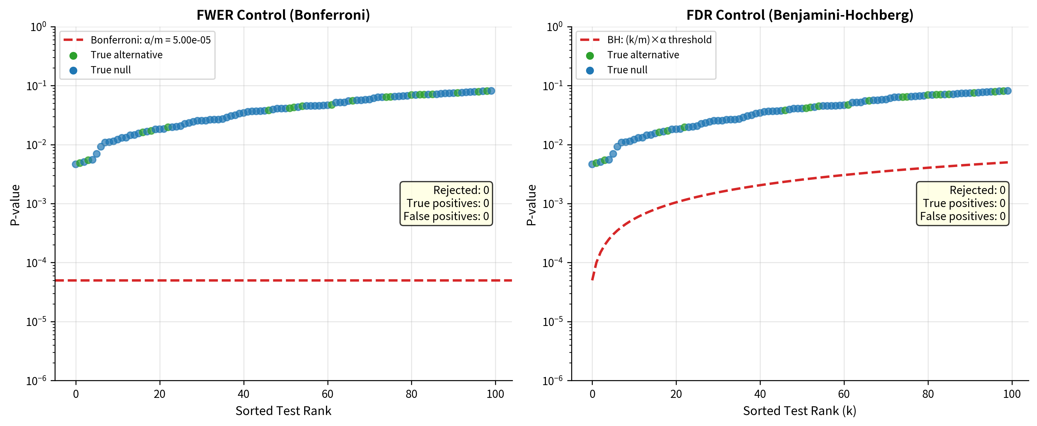
The figure illustrates the key tradeoff:
- Bonferroni (FWER control): Very conservative threshold rejects only the strongest signals, minimizing false positives but missing many true effects
- Benjamini-Hochberg (FDR control): Less stringent threshold detects more true effects at the cost of accepting some false positives
FWER-Controlling Methods
Bonferroni Correction
The Bonferroni correction is the simplest and most widely known method for controlling FWER. The idea is mathematically elegant: if you want the overall error rate to be at most across tests, make each individual test more stringent.
The method: To test hypotheses while controlling FWER at level :
- Reject hypothesis if
- Equivalently, compute adjusted p-values:
Mathematical justification: The Bonferroni inequality states that for any events :
Let be the event that test produces a false positive. If we use threshold for each test:
Properties:
- Always valid (makes no assumptions about test dependence)
- Very conservative, especially for large
- Power decreases as increases
- Simple to implement and explain
Šidák Correction
The Šidák correction is slightly less conservative than Bonferroni and is exact when tests are independent.
The method: For independent tests at FWER level :
- Reject hypothesis if
Mathematical justification: If tests are independent and we want FWER = :
Solving for the per-test significance level:
Comparison with Bonferroni: For tests at :
- Bonferroni:
- Šidák:
The difference is small but Šidák is slightly more powerful. However, Šidák requires independence while Bonferroni is always valid.
Holm's Step-Down Procedure
Holm's method (1979) is uniformly more powerful than Bonferroni while still controlling FWER. The key insight is that we can be less stringent on tests with larger p-values.
The algorithm:
- Order p-values:
- For :
- If , stop and reject all hypotheses with smaller p-values
- Otherwise, continue to the next p-value
- If all p-values pass their thresholds, reject all hypotheses
Mathematical justification: The adjusted thresholds form a step-down sequence:
The first comparison uses the Bonferroni threshold, but subsequent comparisons are less stringent. This maintains FWER control because once we fail to reject at step , we know that hypothesis has , and remaining hypotheses have even larger p-values.
Hochberg's Step-Up Procedure
Hochberg's method (1988) is similar to Holm but works in the opposite direction (step-up instead of step-down). It's more powerful than Holm but requires the assumption that tests are independent or positively correlated.
The algorithm:
- Order p-values:
- For (starting from largest):
- If , reject all hypotheses with p-values
- Otherwise, continue to the next smaller p-value
When to use:
- When tests are independent or positively correlated
- When you want more power than Holm
- Not valid for negatively correlated tests
Comparing FWER Methods

FDR-Controlling Methods
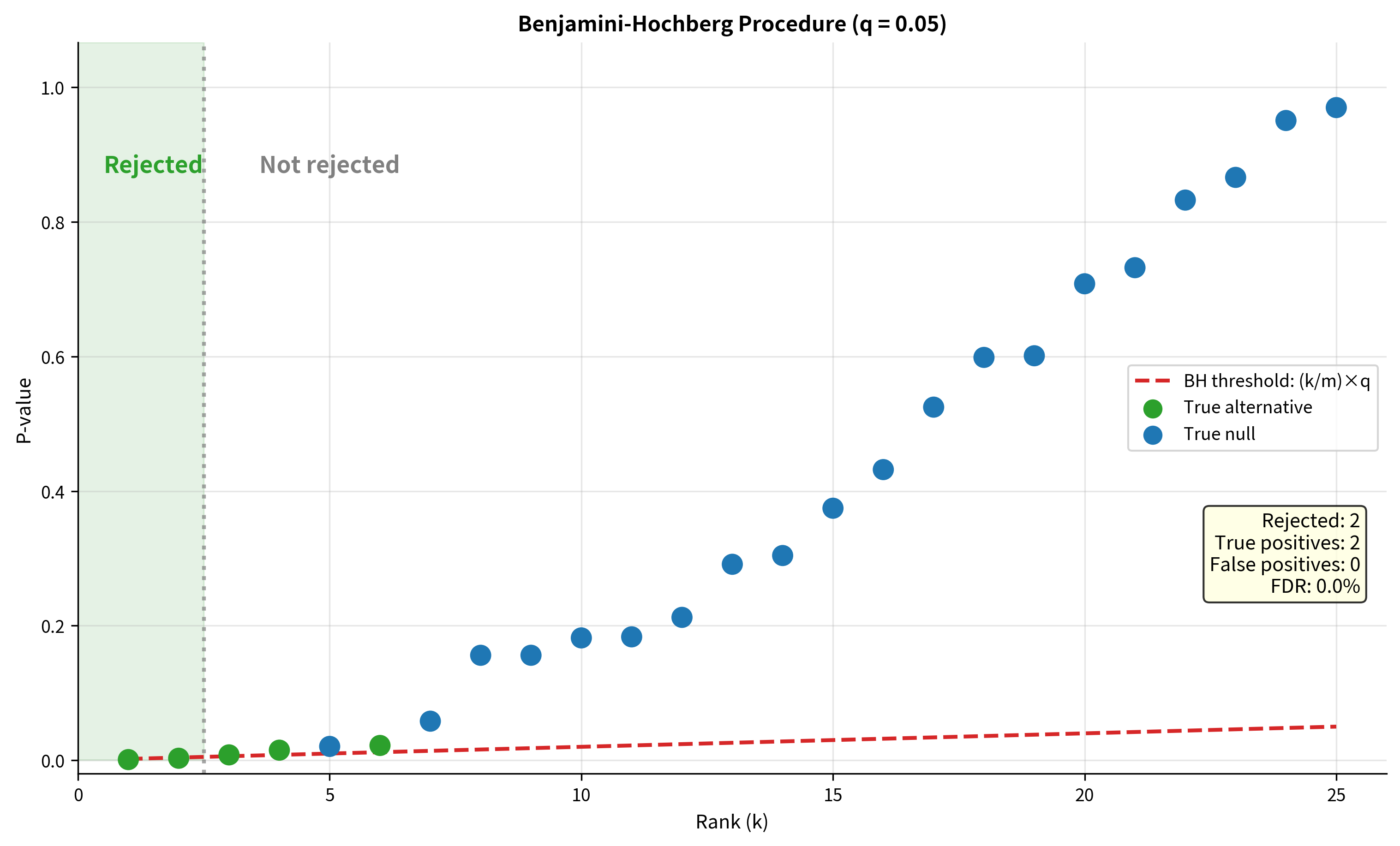
Benjamini-Hochberg Procedure
The Benjamini-Hochberg (BH) procedure (1995) is the most widely used method for controlling the false discovery rate. It's less conservative than FWER methods, allowing more discoveries while controlling the expected proportion of false positives among rejected hypotheses.
The algorithm:
- Order p-values:
- Find the largest such that (where is the desired FDR level)
- Reject all hypotheses with p-values
Mathematical justification: The BH procedure controls FDR at level under the assumption that the test statistics are independent (or positively dependent under some conditions). The key insight is that the threshold increases with rank, allowing more rejections among the smaller p-values.
Adjusted p-values: The BH-adjusted p-value for the hypothesis with rank is:
This ensures monotonicity: if , then .
Benjamini-Yekutieli Procedure
The Benjamini-Yekutieli (BY) procedure (2001) extends BH to handle arbitrary dependence structures among tests. It's more conservative than BH but valid under any dependence.
The method: Replace the BH threshold with , where:
This correction factor accounts for potential negative correlations among tests.
Visualizing the BH Procedure
Post-Hoc Tests for ANOVA
When ANOVA reveals significant differences among groups, post-hoc tests determine which specific pairs differ. These are inherently multiple comparison problems since comparing groups involves pairwise comparisons.
Tukey's Honest Significant Difference (HSD)
Tukey's HSD is the most common post-hoc test for ANOVA. It controls the family-wise error rate for all pairwise comparisons when group sizes are equal.
The method: Two groups and are significantly different if:
where:
- is the critical value from the Studentized Range distribution
- is the number of groups
- is the within-groups degrees of freedom
- is the within-groups mean square (from ANOVA)
- is the sample size per group
When to use:
- All pairwise comparisons are of interest
- Equal (or approximately equal) sample sizes
- Homogeneity of variance assumption met
Dunnett's Test
Dunnett's test compares each treatment group to a single control group. It's more powerful than Tukey's HSD when you only care about comparisons with the control.
When to use:
- One group is a control/reference
- Only comparisons with control are of interest
- More powerful than Tukey for this specific situation
Scheffé's Method
Scheffé's method is the most flexible but also most conservative post-hoc test. It controls FWER for all possible contrasts (not just pairwise comparisons), including complex comparisons like "Group A vs. the average of Groups B and C."
When to use:
- Unplanned (post-hoc) comparisons
- Complex contrasts beyond simple pairwise comparisons
- Unequal sample sizes
- Most conservative option
Summary of Post-Hoc Methods
| Method | Comparisons | Sample Sizes | Power | Use Case |
|---|---|---|---|---|
| Tukey HSD | All pairwise | Equal | Moderate | Standard choice for all pairwise |
| Bonferroni | Any | Any | Low | Simple, always valid |
| Holm | Any | Any | Moderate | Better than Bonferroni |
| Dunnett | vs. Control only | Any | High | Treatment vs. control |
| Scheffé | Any contrast | Any | Low | Complex, unplanned contrasts |
Practical Implementation with scipy.stats
Let's work through a complete example using scipy's built-in multiple comparison functions.
Comparing Methods on Real-World Scale

Common Pitfalls and Best Practices
Pitfall 1: Ignoring Multiple Comparisons
The most serious pitfall is ignoring the multiple comparisons problem entirely. This leads to inflated false positive rates and unreliable conclusions.
Multiple comparisons can be hidden in various ways:
- Testing many subgroups without pre-specification
- Analyzing data at multiple time points
- Testing multiple outcomes without correction
- "Peeking" at data during sequential data collection
- Testing different model specifications
All of these constitute multiple testing and require appropriate correction.
Pitfall 2: Overcorrecting
Applying overly conservative corrections (like Bonferroni when BH would suffice) reduces power and may cause you to miss real effects. Match your correction method to your research goals.
Pitfall 3: Correcting Within Correlated Families
When tests are strongly positively correlated (e.g., testing the same hypothesis in overlapping subsamples), standard corrections become overly conservative. Consider methods designed for dependent tests or reduce to independent tests.
Best Practices
- Pre-specify your analysis plan: Define which tests you'll conduct before seeing the data
- Match correction to research phase: Use FWER for confirmatory research, FDR for exploratory
- Report the correction method used: Always state which correction you applied
- Report both raw and adjusted p-values: Allows readers to apply their own standards
- Consider the dependence structure: Use BH for independent/positive dependence, BY for arbitrary dependence
- Focus on effect sizes: A barely significant corrected p-value with a tiny effect size isn't very informative
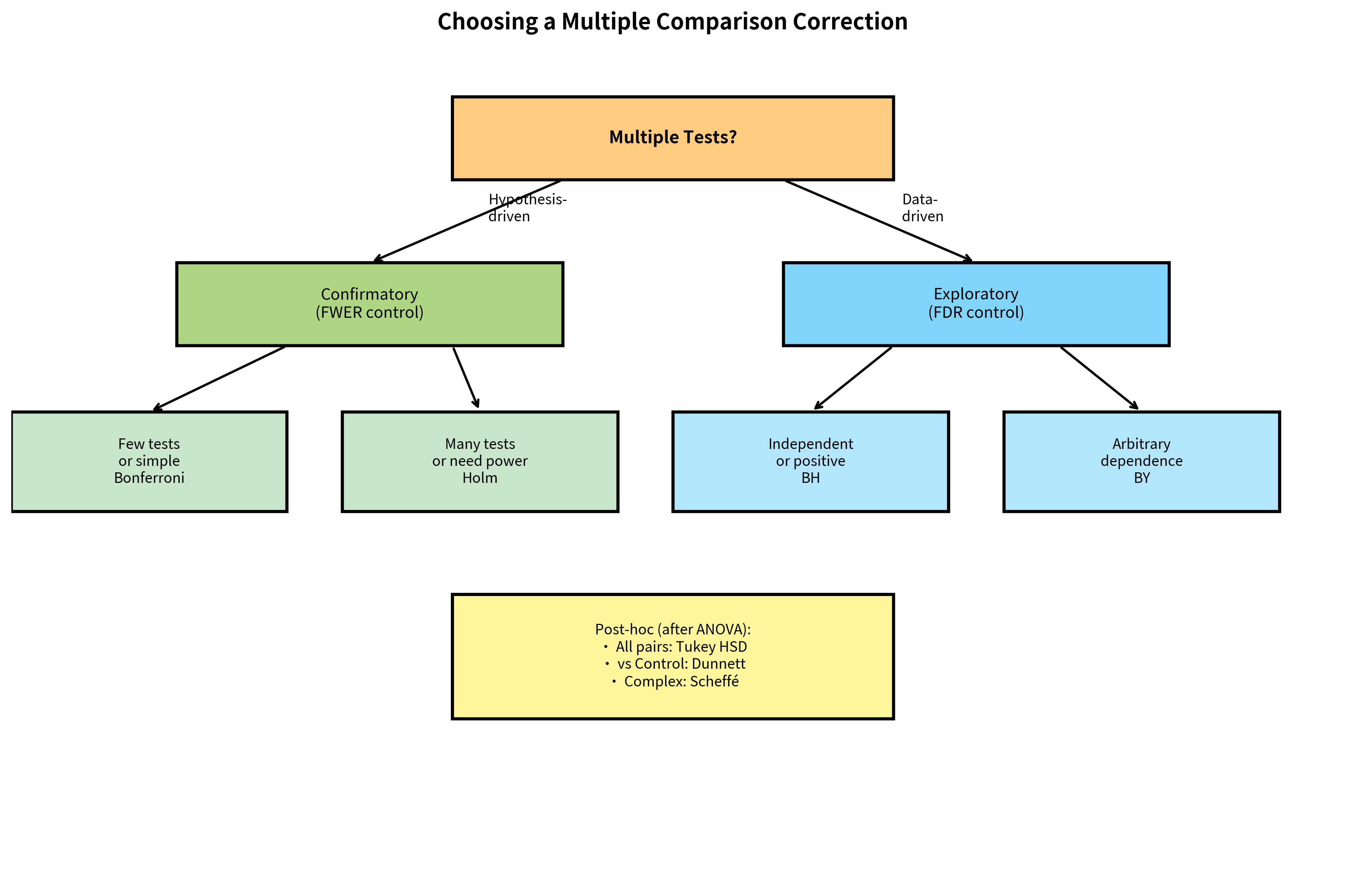
Decision Framework
Summary
The multiple comparisons problem is one of the most important concepts in modern statistics. When conducting many hypothesis tests, the probability of false positives increases dramatically: from 5% for a single test to 99.4% for 100 tests at .
Key concepts:
- Family-wise error rate (FWER): Probability of at least one false positive; controlled by Bonferroni, Šidák, Holm, Hochberg
- False discovery rate (FDR): Expected proportion of false positives among rejections; controlled by Benjamini-Hochberg, Benjamini-Yekutieli
- FWER methods are more conservative, appropriate for confirmatory research
- FDR methods allow more discoveries, appropriate for exploratory research
Correction methods:
| Method | Controls | Power | Assumptions |
|---|---|---|---|
| Bonferroni | FWER | Low | None |
| Šidák | FWER | Low-Moderate | Independence |
| Holm | FWER | Moderate | None |
| Hochberg | FWER | Moderate-High | Independence/positive dependence |
| BH | FDR | High | Independence/positive dependence |
| BY | FDR | Moderate | None |
For ANOVA post-hoc tests:
- Tukey HSD for all pairwise comparisons
- Dunnett for comparisons with control
- Scheffé for complex contrasts
The dead salmon study reminds us that even absurd results can appear "significant" when we conduct enough tests without correction. Proper handling of multiple comparisons is essential for valid statistical inference.
What's Next
This chapter has covered the multiple comparisons problem and methods for controlling error rates when conducting many tests. You've learned the distinction between FWER and FDR, implemented correction methods from Bonferroni to Benjamini-Hochberg, and explored post-hoc tests for ANOVA.
In the final chapter of this series, we'll bring together all the concepts from hypothesis testing into a comprehensive practical guide. You'll find reference tables, decision frameworks, reporting guidelines, and a complete workflow for conducting hypothesis tests in practice: everything you need to apply these concepts to real data analysis.
Quiz
Ready to test your understanding? Take this quick quiz to reinforce what you've learned about multiple comparisons and false discovery control.

Comments