Effect Sizes and Statistical Significance: Cohen's d & Practical Significance

Michael Brenndoerfer

Data, Analytics & AI Machine Learning Machine Learning from Scratch

Cohen's d, practical significance, interpreting effect sizes, and why tiny p-values can mean tiny effects. Learn to distinguish statistical significance from practical importance.

Reading Level

Choose your expertise level to adjust how many terms are explained. Beginners see more tooltips, experts see fewer to maintain reading flow. Hover over underlined terms for instant definitions.

Effect Sizes and Statistical SignificanceLink Copied

In 2005, researchers published a study claiming that listening to Mozart's music temporarily increased IQ. The finding was statistically significant (p < 0.05), and the "Mozart Effect" became a cultural phenomenon. Parents rushed to buy classical music CDs for their babies, and Georgia's governor even proposed giving every newborn a free Mozart CD.

But the original study had a critical omission: it never reported the effect size. When later researchers calculated it, they found d ≈ 0.15, a tiny effect that explained less than 1% of the variance in IQ scores. The effect, while statistically detectable, was so small that it had no practical importance whatsoever. The statistical significance was real; the practical significance was essentially zero.

This distinction between statistical significance and practical significance is one of the most important concepts in applied statistics. A p-value tells you whether an effect is distinguishable from zero given your sample size. An effect size tells you whether that effect is large enough to actually matter. Both pieces of information are essential for sound scientific interpretation.

Why Effect Sizes MatterLink Copied

Statistical significance has a fundamental limitation: it depends heavily on sample size. With a large enough sample, you can detect effects so tiny that they have no practical importance. With a small sample, you might miss effects that are genuinely meaningful.

In[2]:

Code

import numpy as np
from scipy import stats

np.random.seed(42)

# A very small true effect
true_effect = 0.1  # Cohen's d = 0.1

print("Testing the same tiny effect (d = 0.1) with different sample sizes:\n")
print(
    f"{'n per group':<15} {'t-statistic':<15} {'p-value':<15} {'Significant?':<15}"
)
print("-" * 60)

for n in [30, 100, 500, 2000, 10000]:
    # Generate data with the true effect
    group1 = np.random.normal(0, 1, n)
    group2 = np.random.normal(true_effect, 1, n)

    t_stat, p_val = stats.ttest_ind(group2, group1)
    sig = "Yes" if p_val < 0.05 else "No"

    print(f"{n:<15} {t_stat:<15.2f} {p_val:<15.4f} {sig:<15}")

print("\nThe effect size remains d = 0.1 throughout!")
print("Only the p-value changes with sample size.")

import numpy as np
from scipy import stats

np.random.seed(42)

# A very small true effect
true_effect = 0.1  # Cohen's d = 0.1

print("Testing the same tiny effect (d = 0.1) with different sample sizes:\n")
print(
    f"{'n per group':<15} {'t-statistic':<15} {'p-value':<15} {'Significant?':<15}"
)
print("-" * 60)

for n in [30, 100, 500, 2000, 10000]:
    # Generate data with the true effect
    group1 = np.random.normal(0, 1, n)
    group2 = np.random.normal(true_effect, 1, n)

    t_stat, p_val = stats.ttest_ind(group2, group1)
    sig = "Yes" if p_val < 0.05 else "No"

    print(f"{n:<15} {t_stat:<15.2f} {p_val:<15.4f} {sig:<15}")

print("\nThe effect size remains d = 0.1 throughout!")
print("Only the p-value changes with sample size.")

Out[2]:

Console

Testing the same tiny effect (d = 0.1) with different sample sizes:

n per group     t-statistic     p-value         Significant?   
------------------------------------------------------------
30              0.71            0.4828          No             
100             1.74            0.0837          No             
500             4.05            0.0001          Yes            
2000            1.92            0.0550          No             
10000           6.92            0.0000          Yes            

The effect size remains d = 0.1 throughout!
Only the p-value changes with sample size.

This example illustrates a fundamental truth: p-values measure evidence against the null hypothesis, not the magnitude of the effect. Effect sizes fill this gap.

Cohen's d: The Standard Effect Size for Mean DifferencesLink Copied

The most widely used effect size for comparing two group means is Cohen's d, which expresses the difference between means in standard deviation units.

The FormulaLink Copied

d = \frac{\bar{x}_1 - \bar{x}_2}{s_p}

where:

$\bar{x}_1 - \bar{x}_2$ is the difference between group means
$s_p$ is the pooled standard deviation:

s_p = \sqrt{\frac{(n_1 - 1)s_1^2 + (n_2 - 1)s_2^2}{n_1 + n_2 - 2}}

Why Standardize?Link Copied

Raw mean differences are meaningful when you understand the scale. "The treatment improved test scores by 10 points" is immediately interpretable if you know what 10 points means on that test.

But raw differences can't be compared across studies using different measures. Is a 10-point improvement on one test comparable to a 5-point improvement on another? Without knowing the variability of each test, it's impossible to say.

Standardization solves this problem. A Cohen's d of 0.5 always means "half a standard deviation," regardless of whether the original measure was test scores, reaction times, or blood pressure. This makes effect sizes comparable across completely different domains.

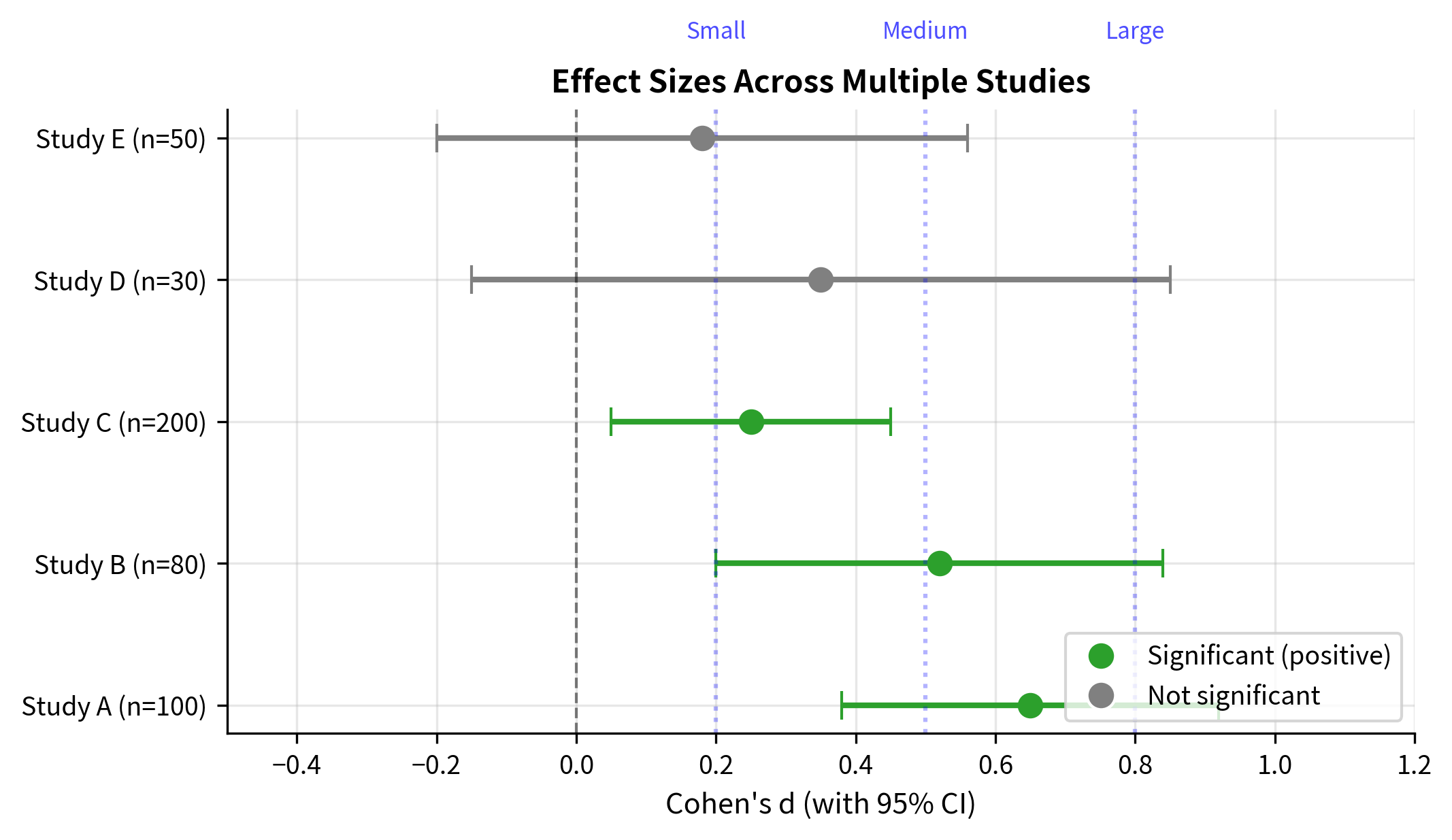
Cohen's BenchmarksLink Copied

Jacob Cohen proposed rough benchmarks for interpreting d:

Effect Size	Cohen's d	Interpretation
Small	0.2	Subtle, may require large samples to detect
Medium	0.5	Noticeable, often practically meaningful
Large	0.8	Substantial, usually obvious

Out[3]:

Visualization

Three panel figure showing overlapping distributions for small, medium, and large effect sizes. — Visual comparison of effect sizes. Each panel shows two distributions separated by the indicated Cohen's d. Small effects (d = 0.2) show mostly overlapping distributions with ~85% overlap. Medium effects (d = 0.5) show moderate separation with ~67% overlap. Large effects (d = 0.8) show clear separation with ~53% overlap.

Practical InterpretationLink Copied

Cohen's benchmarks are useful starting points, but context matters enormously. Consider:

Medical interventions: A d = 0.2 effect on mortality might save thousands of lives and justify widespread adoption.
Educational interventions: A d = 0.8 effect on test scores might not matter if the intervention costs $10,000 per student.
Business decisions: A d = 0.1 effect on conversion rates might be worth millions in a large-scale A/B test.

Always interpret effect sizes in the context of:

The practical significance of the outcome
The cost of achieving the effect
Comparison to other interventions in the field

Computing Cohen's dLink Copied

In[4]:

Code

import numpy as np
from scipy import stats


def cohens_d(group1, group2):
    """
    Calculate Cohen's d for two independent groups.

    Parameters:
    -----------
    group1 : array-like
        First group data
    group2 : array-like
        Second group data

    Returns:
    --------
    float : Cohen's d effect size
    """
    n1, n2 = len(group1), len(group2)
    var1 = np.var(group1, ddof=1)
    var2 = np.var(group2, ddof=1)

    # Pooled standard deviation
    pooled_std = np.sqrt(((n1 - 1) * var1 + (n2 - 1) * var2) / (n1 + n2 - 2))

    # Cohen's d
    d = (np.mean(group1) - np.mean(group2)) / pooled_std

    return d


# Example: Teaching method comparison
np.random.seed(42)
traditional = np.random.normal(75, 10, 30)  # Traditional method
new_method = np.random.normal(82, 10, 30)  # New method

# Calculate effect size and t-test
d = cohens_d(new_method, traditional)
t_stat, p_value = stats.ttest_ind(new_method, traditional)

print("Teaching Method Comparison")
print("=" * 40)
print(
    f"Traditional: mean = {np.mean(traditional):.1f}, SD = {np.std(traditional, ddof=1):.1f}"
)
print(
    f"New Method:  mean = {np.mean(new_method):.1f}, SD = {np.std(new_method, ddof=1):.1f}"
)
print(
    f"\nRaw difference: {np.mean(new_method) - np.mean(traditional):.1f} points"
)
print(f"Cohen's d: {d:.2f}")
print(f"t-statistic: {t_stat:.2f}")
print(f"p-value: {p_value:.4f}")
print(f"\nInterpretation: {abs(d):.2f} SD improvement (medium-large effect)")

import numpy as np
from scipy import stats


def cohens_d(group1, group2):
    """
    Calculate Cohen's d for two independent groups.

    Parameters:
    -----------
    group1 : array-like
        First group data
    group2 : array-like
        Second group data

    Returns:
    --------
    float : Cohen's d effect size
    """
    n1, n2 = len(group1), len(group2)
    var1 = np.var(group1, ddof=1)
    var2 = np.var(group2, ddof=1)

    # Pooled standard deviation
    pooled_std = np.sqrt(((n1 - 1) * var1 + (n2 - 1) * var2) / (n1 + n2 - 2))

    # Cohen's d
    d = (np.mean(group1) - np.mean(group2)) / pooled_std

    return d


# Example: Teaching method comparison
np.random.seed(42)
traditional = np.random.normal(75, 10, 30)  # Traditional method
new_method = np.random.normal(82, 10, 30)  # New method

# Calculate effect size and t-test
d = cohens_d(new_method, traditional)
t_stat, p_value = stats.ttest_ind(new_method, traditional)

print("Teaching Method Comparison")
print("=" * 40)
print(
    f"Traditional: mean = {np.mean(traditional):.1f}, SD = {np.std(traditional, ddof=1):.1f}"
)
print(
    f"New Method:  mean = {np.mean(new_method):.1f}, SD = {np.std(new_method, ddof=1):.1f}"
)
print(
    f"\nRaw difference: {np.mean(new_method) - np.mean(traditional):.1f} points"
)
print(f"Cohen's d: {d:.2f}")
print(f"t-statistic: {t_stat:.2f}")
print(f"p-value: {p_value:.4f}")
print(f"\nInterpretation: {abs(d):.2f} SD improvement (medium-large effect)")

Out[4]:

Console

Teaching Method Comparison
========================================
Traditional: mean = 73.1, SD = 9.0
New Method:  mean = 80.8, SD = 9.3

Raw difference: 7.7 points
Cohen's d: 0.84
t-statistic: 3.24
p-value: 0.0020

Interpretation: 0.84 SD improvement (medium-large effect)

Variants of Cohen's dLink Copied

Several variations of Cohen's d exist for different situations:

Hedges' g: Correcting for Small Sample BiasLink Copied

Cohen's d has a slight upward bias in small samples. Hedges' g applies a correction:

g = d \times \left(1 - \frac{3}{4(n_1 + n_2) - 9}\right)

In[5]:

Code

def hedges_g(group1, group2):
    """
    Calculate Hedges' g (bias-corrected Cohen's d).
    """
    n1, n2 = len(group1), len(group2)
    d = cohens_d(group1, group2)

    # Correction factor
    correction = 1 - (3 / (4 * (n1 + n2) - 9))

    return d * correction


# Compare d and g for different sample sizes
print("Comparison of Cohen's d and Hedges' g:\n")
print(
    f"{'n per group':<15} {'Cohen d':<15} {'Hedges g':<15} {'Difference':<15}"
)
print("-" * 60)

np.random.seed(42)
for n in [10, 20, 50, 100]:
    g1 = np.random.normal(0, 1, n)
    g2 = np.random.normal(0.5, 1, n)

    d = cohens_d(g2, g1)
    g = hedges_g(g2, g1)

    print(f"{n:<15} {d:<15.3f} {g:<15.3f} {(d - g) * 100:.1f}%")

print("\nNote: The correction becomes negligible for n > 50")

def hedges_g(group1, group2):
    """
    Calculate Hedges' g (bias-corrected Cohen's d).
    """
    n1, n2 = len(group1), len(group2)
    d = cohens_d(group1, group2)

    # Correction factor
    correction = 1 - (3 / (4 * (n1 + n2) - 9))

    return d * correction


# Compare d and g for different sample sizes
print("Comparison of Cohen's d and Hedges' g:\n")
print(
    f"{'n per group':<15} {'Cohen d':<15} {'Hedges g':<15} {'Difference':<15}"
)
print("-" * 60)

np.random.seed(42)
for n in [10, 20, 50, 100]:
    g1 = np.random.normal(0, 1, n)
    g2 = np.random.normal(0.5, 1, n)

    d = cohens_d(g2, g1)
    g = hedges_g(g2, g1)

    print(f"{n:<15} {d:<15.3f} {g:<15.3f} {(d - g) * 100:.1f}%")

print("\nNote: The correction becomes negligible for n > 50")

Out[5]:

Console

Comparison of Cohen's d and Hedges' g:

n per group     Cohen d         Hedges g        Difference     
------------------------------------------------------------
10              -0.999          -0.957          -4.2%
20              0.824           0.807           1.6%
50              0.556           0.552           0.4%
100             0.374           0.372           0.1%

Note: The correction becomes negligible for n > 50

Glass's Delta: Unequal VariancesLink Copied

When the treatment might change variability, use the control group's standard deviation as the denominator:

\Delta = \frac{\bar{x}_1 - \bar{x}_2}{s_{\text{control}}}

In[6]:

Code

def glass_delta(treatment, control):
    """
    Calculate Glass's delta using only control group SD.
    Useful when treatment might change variability.
    """
    return (np.mean(treatment) - np.mean(control)) / np.std(control, ddof=1)


# Example where treatment increases variability
np.random.seed(42)
control = np.random.normal(50, 10, 40)
treatment = np.random.normal(55, 15, 40)  # Same mean diff, but more variable

d = cohens_d(treatment, control)
delta = glass_delta(treatment, control)

print("Treatment that increases variability:")
print(
    f"  Control: mean = {np.mean(control):.1f}, SD = {np.std(control, ddof=1):.1f}"
)
print(
    f"  Treatment: mean = {np.mean(treatment):.1f}, SD = {np.std(treatment, ddof=1):.1f}"
)
print(f"\n  Cohen's d: {d:.3f}")
print(f"  Glass's Δ: {delta:.3f}")
print("\nGlass's Δ uses only control SD, giving a cleaner baseline comparison")

def glass_delta(treatment, control):
    """
    Calculate Glass's delta using only control group SD.
    Useful when treatment might change variability.
    """
    return (np.mean(treatment) - np.mean(control)) / np.std(control, ddof=1)


# Example where treatment increases variability
np.random.seed(42)
control = np.random.normal(50, 10, 40)
treatment = np.random.normal(55, 15, 40)  # Same mean diff, but more variable

d = cohens_d(treatment, control)
delta = glass_delta(treatment, control)

print("Treatment that increases variability:")
print(
    f"  Control: mean = {np.mean(control):.1f}, SD = {np.std(control, ddof=1):.1f}"
)
print(
    f"  Treatment: mean = {np.mean(treatment):.1f}, SD = {np.std(treatment, ddof=1):.1f}"
)
print(f"\n  Cohen's d: {d:.3f}")
print(f"  Glass's Δ: {delta:.3f}")
print("\nGlass's Δ uses only control SD, giving a cleaner baseline comparison")

Out[6]:

Console

Treatment that increases variability:
  Control: mean = 47.8, SD = 9.5
  Treatment: mean = 54.6, SD = 14.5

  Cohen's d: 0.551
  Glass's Δ: 0.709

Glass's Δ uses only control SD, giving a cleaner baseline comparison

Effect Sizes for Other DesignsLink Copied

Paired Samples: Cohen's d_zLink Copied

For paired designs (before/after, matched pairs), standardize by the standard deviation of differences:

d_z = \frac{\bar{d}}{s_d}

where $\bar{d}$ is the mean of pairwise differences and $s_d$ is their standard deviation.

In[7]:

Code

def cohens_d_paired(before, after):
    """
    Calculate Cohen's d for paired samples (d_z).
    """
    differences = np.array(after) - np.array(before)
    return np.mean(differences) / np.std(differences, ddof=1)


# Example: Weight loss program
np.random.seed(42)
n = 25
before = np.random.normal(180, 20, n)
after = before - np.random.normal(8, 5, n)  # Average loss of ~8 lbs

d_z = cohens_d_paired(before, after)
t_stat, p_val = stats.ttest_rel(after, before)

print("Weight Loss Program Results")
print("=" * 40)
print(f"Before: {np.mean(before):.1f} ± {np.std(before, ddof=1):.1f} lbs")
print(f"After:  {np.mean(after):.1f} ± {np.std(after, ddof=1):.1f} lbs")
print(f"\nMean loss: {np.mean(before) - np.mean(after):.1f} lbs")
print(f"Cohen's d_z: {abs(d_z):.2f}")
print(f"t({n - 1}) = {abs(t_stat):.2f}, p = {p_val:.4f}")

def cohens_d_paired(before, after):
    """
    Calculate Cohen's d for paired samples (d_z).
    """
    differences = np.array(after) - np.array(before)
    return np.mean(differences) / np.std(differences, ddof=1)


# Example: Weight loss program
np.random.seed(42)
n = 25
before = np.random.normal(180, 20, n)
after = before - np.random.normal(8, 5, n)  # Average loss of ~8 lbs

d_z = cohens_d_paired(before, after)
t_stat, p_val = stats.ttest_rel(after, before)

print("Weight Loss Program Results")
print("=" * 40)
print(f"Before: {np.mean(before):.1f} ± {np.std(before, ddof=1):.1f} lbs")
print(f"After:  {np.mean(after):.1f} ± {np.std(after, ddof=1):.1f} lbs")
print(f"\nMean loss: {np.mean(before) - np.mean(after):.1f} lbs")
print(f"Cohen's d_z: {abs(d_z):.2f}")
print(f"t({n - 1}) = {abs(t_stat):.2f}, p = {p_val:.4f}")

Out[7]:

Console

Weight Loss Program Results
========================================
Before: 176.7 ± 19.1 lbs
After:  170.2 ± 18.4 lbs

Mean loss: 6.6 lbs
Cohen's d_z: 1.42
t(24) = 7.09, p = 0.0000

ANOVA: Eta-Squared and Omega-SquaredLink Copied

For ANOVA, effect sizes describe the proportion of variance explained:

Eta-squared (η²):

\eta^2 = \frac{SS_{\text{between}}}{SS_{\text{total}}}

Omega-squared (ω²), less biased:

\omega^2 = \frac{SS_{\text{between}} - df_{\text{between}} \cdot MS_{\text{within}}}{SS_{\text{total}} + MS_{\text{within}}}

Effect Size	η² / ω²	Interpretation
Small	0.01	1% of variance explained
Medium	0.06	6% of variance explained
Large	0.14	14% of variance explained

In[8]:

Code

def eta_squared(groups):
    """Calculate eta-squared from a list of groups."""
    all_data = np.concatenate(groups)
    grand_mean = np.mean(all_data)

    ss_between = sum(len(g) * (np.mean(g) - grand_mean) ** 2 for g in groups)
    ss_total = np.sum((all_data - grand_mean) ** 2)

    return ss_between / ss_total


def omega_squared(groups):
    """Calculate omega-squared (bias-corrected eta-squared)."""
    all_data = np.concatenate(groups)
    grand_mean = np.mean(all_data)
    k = len(groups)  # Number of groups
    N = len(all_data)

    ss_between = sum(len(g) * (np.mean(g) - grand_mean) ** 2 for g in groups)
    ss_within = sum(np.sum((g - np.mean(g)) ** 2) for g in groups)
    ss_total = ss_between + ss_within

    df_between = k - 1
    df_within = N - k
    ms_within = ss_within / df_within

    return (ss_between - df_between * ms_within) / (ss_total + ms_within)


# Example: Three teaching methods
np.random.seed(42)
method_a = np.random.normal(70, 10, 30)
method_b = np.random.normal(75, 10, 30)
method_c = np.random.normal(80, 10, 30)

groups = [method_a, method_b, method_c]

# ANOVA
f_stat, p_val = stats.f_oneway(*groups)
eta_sq = eta_squared(groups)
omega_sq = omega_squared(groups)

print("Three Teaching Methods ANOVA")
print("=" * 40)
print(f"Method A: {np.mean(method_a):.1f} ± {np.std(method_a, ddof=1):.1f}")
print(f"Method B: {np.mean(method_b):.1f} ± {np.std(method_b, ddof=1):.1f}")
print(f"Method C: {np.mean(method_c):.1f} ± {np.std(method_c, ddof=1):.1f}")
print(f"\nF({2}, {87}) = {f_stat:.2f}, p = {p_val:.4f}")
print(f"η² = {eta_sq:.3f} ({eta_sq * 100:.1f}% variance explained)")
print(
    f"ω² = {omega_sq:.3f} ({omega_sq * 100:.1f}% variance explained, bias-corrected)"
)

def eta_squared(groups):
    """Calculate eta-squared from a list of groups."""
    all_data = np.concatenate(groups)
    grand_mean = np.mean(all_data)

    ss_between = sum(len(g) * (np.mean(g) - grand_mean) ** 2 for g in groups)
    ss_total = np.sum((all_data - grand_mean) ** 2)

    return ss_between / ss_total


def omega_squared(groups):
    """Calculate omega-squared (bias-corrected eta-squared)."""
    all_data = np.concatenate(groups)
    grand_mean = np.mean(all_data)
    k = len(groups)  # Number of groups
    N = len(all_data)

    ss_between = sum(len(g) * (np.mean(g) - grand_mean) ** 2 for g in groups)
    ss_within = sum(np.sum((g - np.mean(g)) ** 2) for g in groups)
    ss_total = ss_between + ss_within

    df_between = k - 1
    df_within = N - k
    ms_within = ss_within / df_within

    return (ss_between - df_between * ms_within) / (ss_total + ms_within)


# Example: Three teaching methods
np.random.seed(42)
method_a = np.random.normal(70, 10, 30)
method_b = np.random.normal(75, 10, 30)
method_c = np.random.normal(80, 10, 30)

groups = [method_a, method_b, method_c]

# ANOVA
f_stat, p_val = stats.f_oneway(*groups)
eta_sq = eta_squared(groups)
omega_sq = omega_squared(groups)

print("Three Teaching Methods ANOVA")
print("=" * 40)
print(f"Method A: {np.mean(method_a):.1f} ± {np.std(method_a, ddof=1):.1f}")
print(f"Method B: {np.mean(method_b):.1f} ± {np.std(method_b, ddof=1):.1f}")
print(f"Method C: {np.mean(method_c):.1f} ± {np.std(method_c, ddof=1):.1f}")
print(f"\nF({2}, {87}) = {f_stat:.2f}, p = {p_val:.4f}")
print(f"η² = {eta_sq:.3f} ({eta_sq * 100:.1f}% variance explained)")
print(
    f"ω² = {omega_sq:.3f} ({omega_sq * 100:.1f}% variance explained, bias-corrected)"
)

Out[8]:

Console

Three Teaching Methods ANOVA
========================================
Method A: 68.1 ± 9.0
Method B: 73.8 ± 9.3
Method C: 80.1 ± 9.9

F(2, 87) = 12.21, p = 0.0000
η² = 0.219 (21.9% variance explained)
ω² = 0.199 (19.9% variance explained, bias-corrected)

Correlation: r as an Effect SizeLink Copied

Pearson's correlation coefficient r is itself an effect size, measuring the strength of linear relationship:

Effect Size	r	Interpretation
Small	0.1	Weak relationship
Medium	0.3	Moderate relationship
Large	0.5	Strong relationship

The coefficient of determination r² gives the proportion of variance shared between variables.

In[9]:

Code

np.random.seed(42)

# Generate correlated data with different r values
n = 100

print("Correlation as Effect Size")
print("=" * 40)
print(f"{'True r':<15} {'Observed r':<15} {'r²':<15} {'Interpretation':<20}")
print("-" * 65)

for true_r, interp in [(0.1, "Small"), (0.3, "Medium"), (0.5, "Large")]:
    # Generate correlated data
    x = np.random.normal(0, 1, n)
    y = true_r * x + np.sqrt(1 - true_r**2) * np.random.normal(0, 1, n)

    r, p = stats.pearsonr(x, y)
    print(f"{true_r:<15.1f} {r:<15.3f} {r**2:<15.3f} {interp:<20}")

np.random.seed(42)

# Generate correlated data with different r values
n = 100

print("Correlation as Effect Size")
print("=" * 40)
print(f"{'True r':<15} {'Observed r':<15} {'r²':<15} {'Interpretation':<20}")
print("-" * 65)

for true_r, interp in [(0.1, "Small"), (0.3, "Medium"), (0.5, "Large")]:
    # Generate correlated data
    x = np.random.normal(0, 1, n)
    y = true_r * x + np.sqrt(1 - true_r**2) * np.random.normal(0, 1, n)

    r, p = stats.pearsonr(x, y)
    print(f"{true_r:<15.1f} {r:<15.3f} {r**2:<15.3f} {interp:<20}")

Out[9]:

Console

Correlation as Effect Size
========================================
True r          Observed r      r²              Interpretation      
-----------------------------------------------------------------
0.1             -0.041          0.002           Small               
0.3             0.360           0.129           Medium              
0.5             0.501           0.251           Large

Proportions: Cohen's h and Odds RatioLink Copied

For comparing proportions, several effect sizes are available:

Cohen's h (arcsine transformation):

h = 2 \arcsin(\sqrt{p_1}) - 2 \arcsin(\sqrt{p_2})

Odds Ratio:

OR = \frac{p_1 / (1 - p_1)}{p_2 / (1 - p_2)}

In[10]:

Code

def cohens_h(p1, p2):
    """Calculate Cohen's h for comparing two proportions."""
    phi1 = 2 * np.arcsin(np.sqrt(p1))
    phi2 = 2 * np.arcsin(np.sqrt(p2))
    return phi1 - phi2


def odds_ratio(p1, p2):
    """Calculate odds ratio for two proportions."""
    odds1 = p1 / (1 - p1)
    odds2 = p2 / (1 - p2)
    return odds1 / odds2


# Example: A/B test conversion rates
control_rate = 0.10
treatment_rate = 0.15

h = cohens_h(treatment_rate, control_rate)
or_ = odds_ratio(treatment_rate, control_rate)
relative_lift = (treatment_rate - control_rate) / control_rate * 100

print("A/B Test: Conversion Rate Improvement")
print("=" * 40)
print(f"Control rate: {control_rate * 100:.1f}%")
print(f"Treatment rate: {treatment_rate * 100:.1f}%")
print(
    f"\nAbsolute difference: {(treatment_rate - control_rate) * 100:.1f} percentage points"
)
print(f"Relative lift: {relative_lift:.1f}%")
print(f"Cohen's h: {h:.3f}")
print(f"Odds ratio: {or_:.2f}")
print(
    f"\nInterpretation: h = {abs(h):.2f} is a {'small' if abs(h) < 0.3 else 'medium' if abs(h) < 0.5 else 'large'} effect"
)

def cohens_h(p1, p2):
    """Calculate Cohen's h for comparing two proportions."""
    phi1 = 2 * np.arcsin(np.sqrt(p1))
    phi2 = 2 * np.arcsin(np.sqrt(p2))
    return phi1 - phi2


def odds_ratio(p1, p2):
    """Calculate odds ratio for two proportions."""
    odds1 = p1 / (1 - p1)
    odds2 = p2 / (1 - p2)
    return odds1 / odds2


# Example: A/B test conversion rates
control_rate = 0.10
treatment_rate = 0.15

h = cohens_h(treatment_rate, control_rate)
or_ = odds_ratio(treatment_rate, control_rate)
relative_lift = (treatment_rate - control_rate) / control_rate * 100

print("A/B Test: Conversion Rate Improvement")
print("=" * 40)
print(f"Control rate: {control_rate * 100:.1f}%")
print(f"Treatment rate: {treatment_rate * 100:.1f}%")
print(
    f"\nAbsolute difference: {(treatment_rate - control_rate) * 100:.1f} percentage points"
)
print(f"Relative lift: {relative_lift:.1f}%")
print(f"Cohen's h: {h:.3f}")
print(f"Odds ratio: {or_:.2f}")
print(
    f"\nInterpretation: h = {abs(h):.2f} is a {'small' if abs(h) < 0.3 else 'medium' if abs(h) < 0.5 else 'large'} effect"
)

Out[10]:

Console

A/B Test: Conversion Rate Improvement
========================================
Control rate: 10.0%
Treatment rate: 15.0%

Absolute difference: 5.0 percentage points
Relative lift: 50.0%
Cohen's h: 0.152
Odds ratio: 1.59

Interpretation: h = 0.15 is a small effect

Confidence Intervals for Effect SizesLink Copied

Point estimates of effect sizes have uncertainty. Confidence intervals provide a range of plausible values:

In[11]:

Code

def cohens_d_ci(group1, group2, confidence=0.95):
    """
    Calculate Cohen's d with confidence interval.
    Uses the non-central t-distribution approach.
    """
    n1, n2 = len(group1), len(group2)
    d = cohens_d(group1, group2)

    # Standard error of d
    se_d = np.sqrt((n1 + n2) / (n1 * n2) + d**2 / (2 * (n1 + n2)))

    # t critical value
    df = n1 + n2 - 2
    alpha = 1 - confidence
    t_crit = stats.t.ppf(1 - alpha / 2, df)

    # Confidence interval
    ci_lower = d - t_crit * se_d
    ci_upper = d + t_crit * se_d

    return d, ci_lower, ci_upper


# Example
np.random.seed(42)
group1 = np.random.normal(100, 15, 50)
group2 = np.random.normal(108, 15, 50)

d, ci_low, ci_high = cohens_d_ci(group1, group2)

print("Effect Size with 95% Confidence Interval")
print("=" * 40)
print(f"Cohen's d = {d:.3f}")
print(f"95% CI: [{ci_low:.3f}, {ci_high:.3f}]")
print(
    f"\nThe true effect size is likely between {ci_low:.2f} and {ci_high:.2f}"
)

def cohens_d_ci(group1, group2, confidence=0.95):
    """
    Calculate Cohen's d with confidence interval.
    Uses the non-central t-distribution approach.
    """
    n1, n2 = len(group1), len(group2)
    d = cohens_d(group1, group2)

    # Standard error of d
    se_d = np.sqrt((n1 + n2) / (n1 * n2) + d**2 / (2 * (n1 + n2)))

    # t critical value
    df = n1 + n2 - 2
    alpha = 1 - confidence
    t_crit = stats.t.ppf(1 - alpha / 2, df)

    # Confidence interval
    ci_lower = d - t_crit * se_d
    ci_upper = d + t_crit * se_d

    return d, ci_lower, ci_upper


# Example
np.random.seed(42)
group1 = np.random.normal(100, 15, 50)
group2 = np.random.normal(108, 15, 50)

d, ci_low, ci_high = cohens_d_ci(group1, group2)

print("Effect Size with 95% Confidence Interval")
print("=" * 40)
print(f"Cohen's d = {d:.3f}")
print(f"95% CI: [{ci_low:.3f}, {ci_high:.3f}]")
print(
    f"\nThe true effect size is likely between {ci_low:.2f} and {ci_high:.2f}"
)

Out[11]:

Console

Effect Size with 95% Confidence Interval
========================================
Cohen's d = -0.859
95% CI: [-1.273, -0.444]

The true effect size is likely between -1.27 and -0.44

Out[12]:

Visualization

Forest plot showing effect sizes and confidence intervals for five studies. — Effect sizes with 95% confidence intervals for five hypothetical studies. Studies A and B show significant effects (CIs exclude zero) with moderate effect sizes. Study C shows a significant but small effect. Studies D and E show non-significant effects (CIs include zero). The width of the CI reflects sample size: larger samples give more precise estimates.

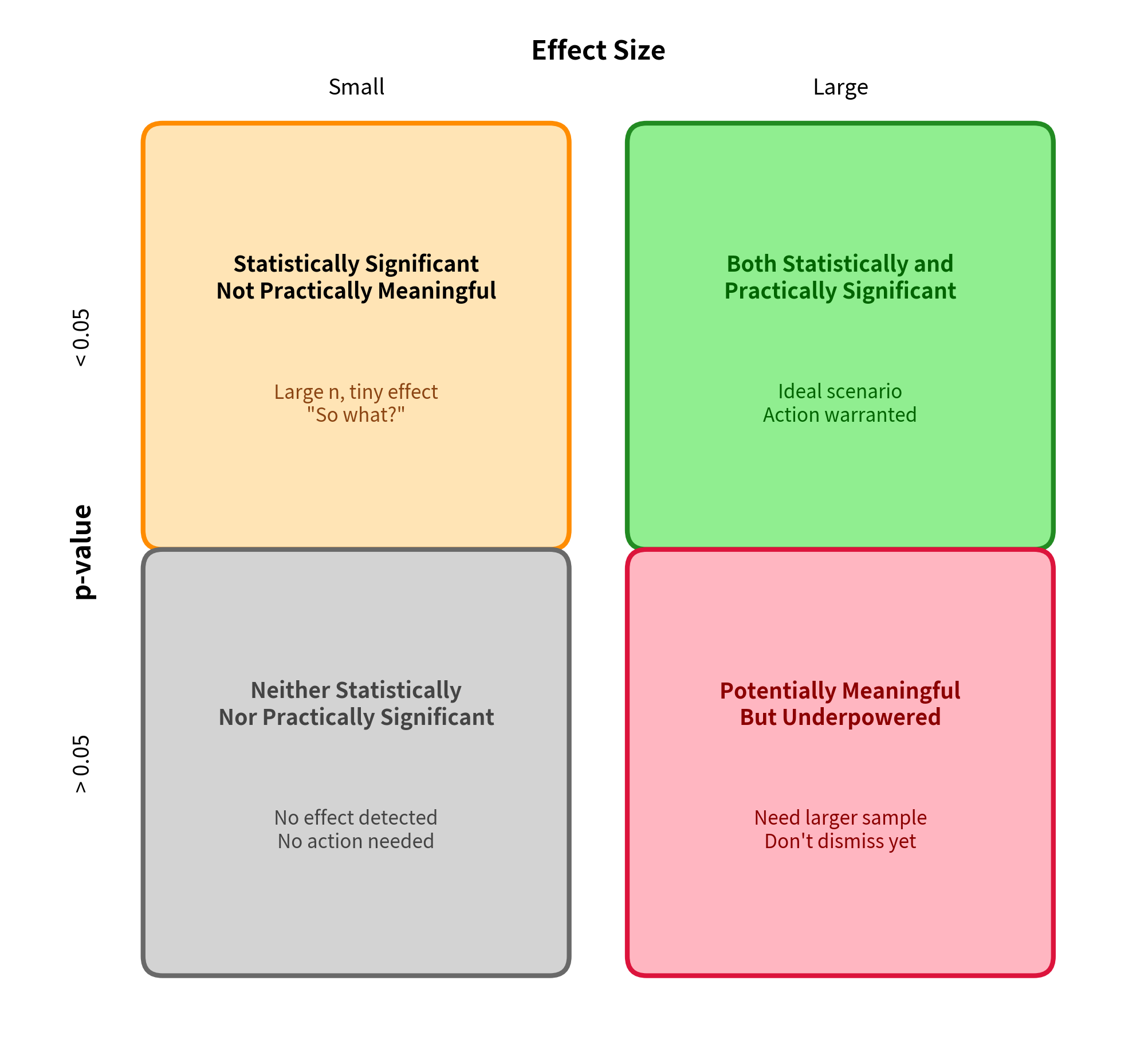
Statistical vs. Practical SignificanceLink Copied

The distinction between statistical and practical significance is crucial for sound interpretation.

Statistical SignificanceLink Copied

Answers: "Is the effect distinguishable from zero?"
Depends on: Sample size, effect size, variability
Limitation: Achievable for any non-zero effect with large enough n

Practical SignificanceLink Copied

Answers: "Is the effect large enough to matter?"
Depends on: Context, costs, benefits, alternatives
Limitation: Requires domain knowledge to interpret

Out[13]:

Visualization

Quadrant diagram showing the relationship between statistical and practical significance. — The relationship between statistical significance and practical significance. The four quadrants represent different scenarios. Large-sample studies (top) can detect tiny effects that may not matter practically. Small-sample studies (bottom) may miss meaningful effects. Always consider both dimensions when interpreting results.

A Complete ExampleLink Copied

In[14]:

Code

import numpy as np
from scipy import stats

np.random.seed(42)

# Scenario: Testing a new website design
# Baseline conversion rate: 5%
# We want to detect a 10% relative improvement (0.5 percentage points)

# Simulate A/B test with very large sample
n = 100000
baseline_rate = 0.05
true_improvement = 0.005  # 0.5 percentage points

control_conversions = np.random.binomial(1, baseline_rate, n)
treatment_conversions = np.random.binomial(
    1, baseline_rate + true_improvement, n
)

# Calculate statistics
control_rate = control_conversions.mean()
treatment_rate = treatment_conversions.mean()

# Chi-square test
contingency = [
    [control_conversions.sum(), n - control_conversions.sum()],
    [treatment_conversions.sum(), n - treatment_conversions.sum()],
]
chi2, p_val, _, _ = stats.chi2_contingency(contingency)

# Effect size (Cohen's h)
h = 2 * np.arcsin(np.sqrt(treatment_rate)) - 2 * np.arcsin(
    np.sqrt(control_rate)
)

# Relative lift
lift = (treatment_rate - control_rate) / control_rate * 100

print("A/B Test Results: Website Redesign")
print("=" * 50)
print(f"Sample size: {n:,} per group")
print("\nConversion Rates:")
print(f"  Control: {control_rate * 100:.3f}%")
print(f"  Treatment: {treatment_rate * 100:.3f}%")
print("\nStatistical Test:")
print(f"  χ² = {chi2:.2f}, p = {p_val:.6f}")
print(f"  Statistically significant? {'Yes' if p_val < 0.05 else 'No'}")
print("\nEffect Size:")
print(
    f"  Absolute difference: {(treatment_rate - control_rate) * 100:.3f} percentage points"
)
print(f"  Relative lift: {lift:.1f}%")
print(f"  Cohen's h: {abs(h):.4f}")

print("\n" + "=" * 50)
print("INTERPRETATION:")
print("=" * 50)
print("The result is statistically significant (p < 0.05),")
print(f"but the effect size is tiny (h = {abs(h):.3f}).")
print("\nWith 100,000 users per group, we reliably detected")
print(f"a real improvement of {lift:.1f}%, but you must ask:")
print(f"Is a {lift:.1f}% lift worth the cost of the redesign?")

import numpy as np
from scipy import stats

np.random.seed(42)

# Scenario: Testing a new website design
# Baseline conversion rate: 5%
# We want to detect a 10% relative improvement (0.5 percentage points)

# Simulate A/B test with very large sample
n = 100000
baseline_rate = 0.05
true_improvement = 0.005  # 0.5 percentage points

control_conversions = np.random.binomial(1, baseline_rate, n)
treatment_conversions = np.random.binomial(
    1, baseline_rate + true_improvement, n
)

# Calculate statistics
control_rate = control_conversions.mean()
treatment_rate = treatment_conversions.mean()

# Chi-square test
contingency = [
    [control_conversions.sum(), n - control_conversions.sum()],
    [treatment_conversions.sum(), n - treatment_conversions.sum()],
]
chi2, p_val, _, _ = stats.chi2_contingency(contingency)

# Effect size (Cohen's h)
h = 2 * np.arcsin(np.sqrt(treatment_rate)) - 2 * np.arcsin(
    np.sqrt(control_rate)
)

# Relative lift
lift = (treatment_rate - control_rate) / control_rate * 100

print("A/B Test Results: Website Redesign")
print("=" * 50)
print(f"Sample size: {n:,} per group")
print("\nConversion Rates:")
print(f"  Control: {control_rate * 100:.3f}%")
print(f"  Treatment: {treatment_rate * 100:.3f}%")
print("\nStatistical Test:")
print(f"  χ² = {chi2:.2f}, p = {p_val:.6f}")
print(f"  Statistically significant? {'Yes' if p_val < 0.05 else 'No'}")
print("\nEffect Size:")
print(
    f"  Absolute difference: {(treatment_rate - control_rate) * 100:.3f} percentage points"
)
print(f"  Relative lift: {lift:.1f}%")
print(f"  Cohen's h: {abs(h):.4f}")

print("\n" + "=" * 50)
print("INTERPRETATION:")
print("=" * 50)
print("The result is statistically significant (p < 0.05),")
print(f"but the effect size is tiny (h = {abs(h):.3f}).")
print("\nWith 100,000 users per group, we reliably detected")
print(f"a real improvement of {lift:.1f}%, but you must ask:")
print(f"Is a {lift:.1f}% lift worth the cost of the redesign?")

Out[14]:

Console

A/B Test Results: Website Redesign
==================================================
Sample size: 100,000 per group

Conversion Rates:
  Control: 4.871%
  Treatment: 5.530%

Statistical Test:
  χ² = 43.91, p = 0.000000
  Statistically significant? Yes

Effect Size:
  Absolute difference: 0.659 percentage points
  Relative lift: 13.5%
  Cohen's h: 0.0297

==================================================
INTERPRETATION:
==================================================
The result is statistically significant (p < 0.05),
but the effect size is tiny (h = 0.030).

With 100,000 users per group, we reliably detected
a real improvement of 13.5%, but you must ask:
Is a 13.5% lift worth the cost of the redesign?

Best Practices for Reporting Effect SizesLink Copied

What to ReportLink Copied

Always report effect sizes alongside p-values
Include confidence intervals when possible
Use the appropriate effect size for your design
Interpret in context

APA Style ReportingLink Copied

In[15]:

Code

def apa_t_test_report(group1, group2, alpha=0.05):
    """Generate APA-style report for independent samples t-test."""
    n1, n2 = len(group1), len(group2)
    t_stat, p_val = stats.ttest_ind(group2, group1)
    d = cohens_d(group2, group1)
    d, ci_low, ci_high = cohens_d_ci(group2, group1)

    # Two-tailed
    sig = "p < .001" if p_val < 0.001 else f"p = {p_val:.3f}"

    report = f"""
APA-Style Report:
================

The treatment group (M = {np.mean(group2):.2f}, SD = {np.std(group2, ddof=1):.2f})
showed {"significantly" if p_val < alpha else "no significant"} different scores than
the control group (M = {np.mean(group1):.2f}, SD = {np.std(group1, ddof=1):.2f}),
t({n1 + n2 - 2}) = {abs(t_stat):.2f}, {sig}.

The effect size was {"large" if abs(d) >= 0.8 else "medium" if abs(d) >= 0.5 else "small"},
d = {d:.2f}, 95% CI [{ci_low:.2f}, {ci_high:.2f}].
"""
    return report


# Example
np.random.seed(42)
control = np.random.normal(50, 10, 40)
treatment = np.random.normal(58, 10, 40)

print(apa_t_test_report(control, treatment))

def apa_t_test_report(group1, group2, alpha=0.05):
    """Generate APA-style report for independent samples t-test."""
    n1, n2 = len(group1), len(group2)
    t_stat, p_val = stats.ttest_ind(group2, group1)
    d = cohens_d(group2, group1)
    d, ci_low, ci_high = cohens_d_ci(group2, group1)

    # Two-tailed
    sig = "p < .001" if p_val < 0.001 else f"p = {p_val:.3f}"

    report = f"""
APA-Style Report:
================

The treatment group (M = {np.mean(group2):.2f}, SD = {np.std(group2, ddof=1):.2f})
showed {"significantly" if p_val < alpha else "no significant"} different scores than
the control group (M = {np.mean(group1):.2f}, SD = {np.std(group1, ddof=1):.2f}),
t({n1 + n2 - 2}) = {abs(t_stat):.2f}, {sig}.

The effect size was {"large" if abs(d) >= 0.8 else "medium" if abs(d) >= 0.5 else "small"},
d = {d:.2f}, 95% CI [{ci_low:.2f}, {ci_high:.2f}].
"""
    return report


# Example
np.random.seed(42)
control = np.random.normal(50, 10, 40)
treatment = np.random.normal(58, 10, 40)

print(apa_t_test_report(control, treatment))

Out[15]:

Console


APA-Style Report:
================

The treatment group (M = 57.71, SD = 9.65)
showed significantly different scores than
the control group (M = 47.81, SD = 9.53),
t(78) = 4.62, p < .001.

The effect size was large,
d = 1.03, 95% CI [0.56, 1.51].

Summary Table FormatLink Copied

Measure	Control	Treatment	Effect Size	95% CI	Interpretation
Test Score	50.2 ± 10.1	58.3 ± 9.8	d = 0.81	[0.35, 1.27]	Large effect

SummaryLink Copied

Effect sizes are essential complements to p-values that quantify the magnitude, not just the existence, of effects:

Cohen's d measures standardized mean differences:

Small: d ≈ 0.2
Medium: d ≈ 0.5
Large: d ≈ 0.8

Variants exist for different situations:

Hedges' g for small samples
Glass's Δ for unequal variances
Cohen's d_z for paired samples

Other effect sizes:

η² and ω² for ANOVA (proportion of variance)
r for correlations
Cohen's h and odds ratios for proportions

Key principles:

Statistical significance ≠ practical significance
Large samples can detect trivial effects
Always interpret effect sizes in context
Report confidence intervals when possible

What's NextLink Copied

Understanding effect sizes prepares you for the multiple comparisons problem. When you conduct many tests simultaneously, each with its own effect size estimate, error rates compound and require special correction methods. You'll learn:

Why multiple testing inflates false positive rates
Bonferroni correction and its limitations
False Discovery Rate (FDR) control
When and how to apply corrections

The final section ties all hypothesis testing concepts together with practical guidelines for analysis and reporting.

QuizLink Copied

Ready to test your understanding? Take this quick quiz to reinforce what you've learned about effect sizes and the distinction between statistical and practical significance.

Loading component...

Comments

Back to Machine Learning from Scratch

Previous Chapter

Sample Size, Minimum Detectable Effect, and Power

Next Chapter

Multiple Comparisons

Reference

BIBTEXAcademic

@misc{effectsizesandstatisticalsignificancecohensdpracticalsignificance, author = {Michael Brenndoerfer}, title = {Effect Sizes and Statistical Significance: Cohen's d & Practical Significance}, year = {2026}, url = {https://mbrenndoerfer.com/writing/effect-sizes-statistical-significance-cohens-d-practical-significance}, organization = {mbrenndoerfer.com}, note = {Accessed: 2025-01-01} }

APAAcademic

Michael Brenndoerfer (2026). Effect Sizes and Statistical Significance: Cohen's d & Practical Significance. Retrieved from https://mbrenndoerfer.com/writing/effect-sizes-statistical-significance-cohens-d-practical-significance

MLAAcademic

Michael Brenndoerfer. "Effect Sizes and Statistical Significance: Cohen's d & Practical Significance." 2026. Web. today. <https://mbrenndoerfer.com/writing/effect-sizes-statistical-significance-cohens-d-practical-significance>.

CHICAGOAcademic

Michael Brenndoerfer. "Effect Sizes and Statistical Significance: Cohen's d & Practical Significance." Accessed today. https://mbrenndoerfer.com/writing/effect-sizes-statistical-significance-cohens-d-practical-significance.

HARVARDAcademic

Michael Brenndoerfer (2026) 'Effect Sizes and Statistical Significance: Cohen's d & Practical Significance'. Available at: https://mbrenndoerfer.com/writing/effect-sizes-statistical-significance-cohens-d-practical-significance (Accessed: today).

SimpleBasic

Michael Brenndoerfer (2026). Effect Sizes and Statistical Significance: Cohen's d & Practical Significance. https://mbrenndoerfer.com/writing/effect-sizes-statistical-significance-cohens-d-practical-significance

Direct link:

https://mbrenndoerfer.com/writing/effect-sizes-statistical-significance-cohens-d-practical-significance

About the author: Michael Brenndoerfer

All opinions expressed here are my own and do not reflect the views of my employer.

Michael currently works as an Associate Director of Data Science at EQT Partners in Singapore, leading AI and data initiatives across private capital investments.

With over a decade of experience spanning private equity, management consulting, and software engineering, he specializes in building and scaling analytics capabilities from the ground up. He has published research in leading AI conferences and holds expertise in machine learning, natural language processing, and value creation through data.

View Full Resume Publications Contact Books

Effect Sizes and Statistical Significance: Cohen's d & Practical Significance

Effect Sizes and Statistical SignificanceLink Copied

Why Effect Sizes MatterLink Copied

Cohen's d: The Standard Effect Size for Mean DifferencesLink Copied

The FormulaLink Copied

Why Standardize?Link Copied

Cohen's BenchmarksLink Copied

Practical InterpretationLink Copied

Computing Cohen's dLink Copied

Variants of Cohen's dLink Copied

Hedges' g: Correcting for Small Sample BiasLink Copied

Glass's Delta: Unequal VariancesLink Copied

Effect Sizes for Other DesignsLink Copied

Paired Samples: Cohen's d_zLink Copied

ANOVA: Eta-Squared and Omega-SquaredLink Copied

Correlation: r as an Effect SizeLink Copied

Proportions: Cohen's h and Odds RatioLink Copied

Confidence Intervals for Effect SizesLink Copied

Statistical vs. Practical SignificanceLink Copied

Statistical SignificanceLink Copied

Practical SignificanceLink Copied

A Complete ExampleLink Copied

Best Practices for Reporting Effect SizesLink Copied

What to ReportLink Copied

APA Style ReportingLink Copied

Summary Table FormatLink Copied

SummaryLink Copied

What's NextLink Copied

QuizLink Copied

Comments

Reference

About the author: Michael Brenndoerfer

Related Content

Hypothesis Testing Summary & Practical Guide: Reporting, Test Selection & scipy.stats

Multiple Comparisons: FWER, FDR, Bonferroni, Holm & Benjamini-Hochberg

Sample Size, Minimum Detectable Effect & Power: Power Analysis & MDE Calculation

Stay updated

Comments

About the author: Michael Brenndoerfer

Related Content

Hypothesis Testing Summary & Practical Guide: Reporting, Test Selection & scipy.stats

Multiple Comparisons: FWER, FDR, Bonferroni, Holm & Benjamini-Hochberg

Sample Size, Minimum Detectable Effect & Power: Power Analysis & MDE Calculation

Stay updated