The F-Test and F-Distribution: Comparing Variances, Regression & Nested Models

Michael BrenndoerferJanuary 4, 202624 min read

F-distribution, F-test for comparing variances, F-test in regression, and nested model comparison. Learn how F-tests extend hypothesis testing beyond means to variance analysis and model comparison.

Reading Level

Choose your expertise level to adjust how many terms are explained. Beginners see more tooltips, experts see fewer to maintain reading flow. Hover over underlined terms for instant definitions.

The F-Test and F-Distribution

So far in this series, we've focused on comparing means: is this sample mean different from a hypothesized value (one-sample t-test)? Do these two groups have different average outcomes (two-sample t-test)? But means tell only part of the story. Two manufacturing processes might produce widgets with the same average diameter, yet one process might be wildly inconsistent while the other is remarkably precise. A financial portfolio might have the same expected return as another, but with far greater volatility. In these cases, variance is what matters.

The F-test addresses questions about variance. Named after Sir Ronald A. Fisher, one of the founders of modern statistics, the F-test emerged from Fisher's work on agricultural experiments in the 1920s. Fisher realized that comparing sources of variation, not just averages, was essential for understanding experimental results. His insights led to both the F-distribution and the Analysis of Variance (ANOVA) framework that revolutionized experimental science.

This chapter introduces the F-distribution and shows how F-tests answer three important types of questions:

  1. Do two populations have equal variance? (Essential for choosing between pooled and Welch's t-tests)
  2. Does a regression model explain significant variation? (Testing overall model significance)
  3. Do additional predictors improve a model? (Comparing nested regression models)

Understanding F-tests here will prepare you for ANOVA, which extends these ideas to compare means across multiple groups by decomposing total variation into components.

Why Compare Variances?

Before diving into the mathematics, let's understand why variance comparisons matter in practice.

Quality control and manufacturing: A factory produces bolts with a target diameter. Two machines might produce bolts with the same average diameter, but if Machine A's output varies by ±0.01\pm 0.01 mm while Machine B's varies by ±0.1\pm 0.1 mm, Machine B will produce far more defective bolts. Comparing variances identifies the less consistent process.

Checking t-test assumptions: The pooled two-sample t-test assumes equal variances between groups. Before using this test, you might want to verify this assumption. The F-test provides a formal way to check.

Investment risk: Two stocks might have the same expected annual return of 8%, but if Stock A has a standard deviation of 5% and Stock B has 25%, they represent very different risk profiles. Comparing variances quantifies this difference.

Measurement precision: When comparing two laboratory instruments or two human raters, you care not just about whether they give the same average reading, but whether one is more variable (less precise) than the other.

The F-Distribution: Where It Comes From

The F-distribution arises naturally when comparing two independent estimates of variance. To understand why, we need to trace through the mathematical foundations.

Building Block: Chi-Squared Distribution

Recall from earlier chapters that when you estimate variance from a sample of nn observations drawn from a normal population with true variance σ2\sigma^2, the quantity:

(n1)s2σ2χn12\frac{(n-1)s^2}{\sigma^2} \sim \chi^2_{n-1}

follows a chi-squared distribution with n1n-1 degrees of freedom. This result reflects the fact that s2s^2 is computed from nn observations but loses one degree of freedom because we estimate the mean from the same data.

From Two Samples to the F-Distribution

Now suppose we have two independent samples from populations with variances σ12\sigma_1^2 and σ22\sigma_2^2:

  • Sample 1: n1n_1 observations, sample variance s12s_1^2
  • Sample 2: n2n_2 observations, sample variance s22s_2^2

Each sample variance, properly scaled, follows a chi-squared distribution:

(n11)s12σ12χn112and(n21)s22σ22χn212\frac{(n_1-1)s_1^2}{\sigma_1^2} \sim \chi^2_{n_1-1} \quad \text{and} \quad \frac{(n_2-1)s_2^2}{\sigma_2^2} \sim \chi^2_{n_2-1}

The F-distribution is defined as the ratio of two independent chi-squared random variables, each divided by its degrees of freedom:

F=χ12/df1χ22/df2F = \frac{\chi_1^2 / df_1}{\chi_2^2 / df_2}

Substituting our variance estimates:

F=s12/σ12s22/σ22=s12s22σ22σ12F = \frac{s_1^2 / \sigma_1^2}{s_2^2 / \sigma_2^2} = \frac{s_1^2}{s_2^2} \cdot \frac{\sigma_2^2}{\sigma_1^2}

The Key Simplification Under the Null Hypothesis

Here's the beautiful part. Under the null hypothesis that σ12=σ22\sigma_1^2 = \sigma_2^2, the ratio σ22/σ12=1\sigma_2^2 / \sigma_1^2 = 1, and we get:

F=s12s22Fdf1,df2F = \frac{s_1^2}{s_2^2} \sim F_{df_1, df_2}

where df1=n11df_1 = n_1 - 1 and df2=n21df_2 = n_2 - 1.

The unknown common variance cancels out! This is why the F-test works: we can test whether two population variances are equal without knowing what those variances actually are. We only need the ratio of the sample variances, and we know its distribution under the null hypothesis.

Properties of the F-Distribution

The F-distribution has distinctive characteristics that set it apart from the normal and t-distributions:

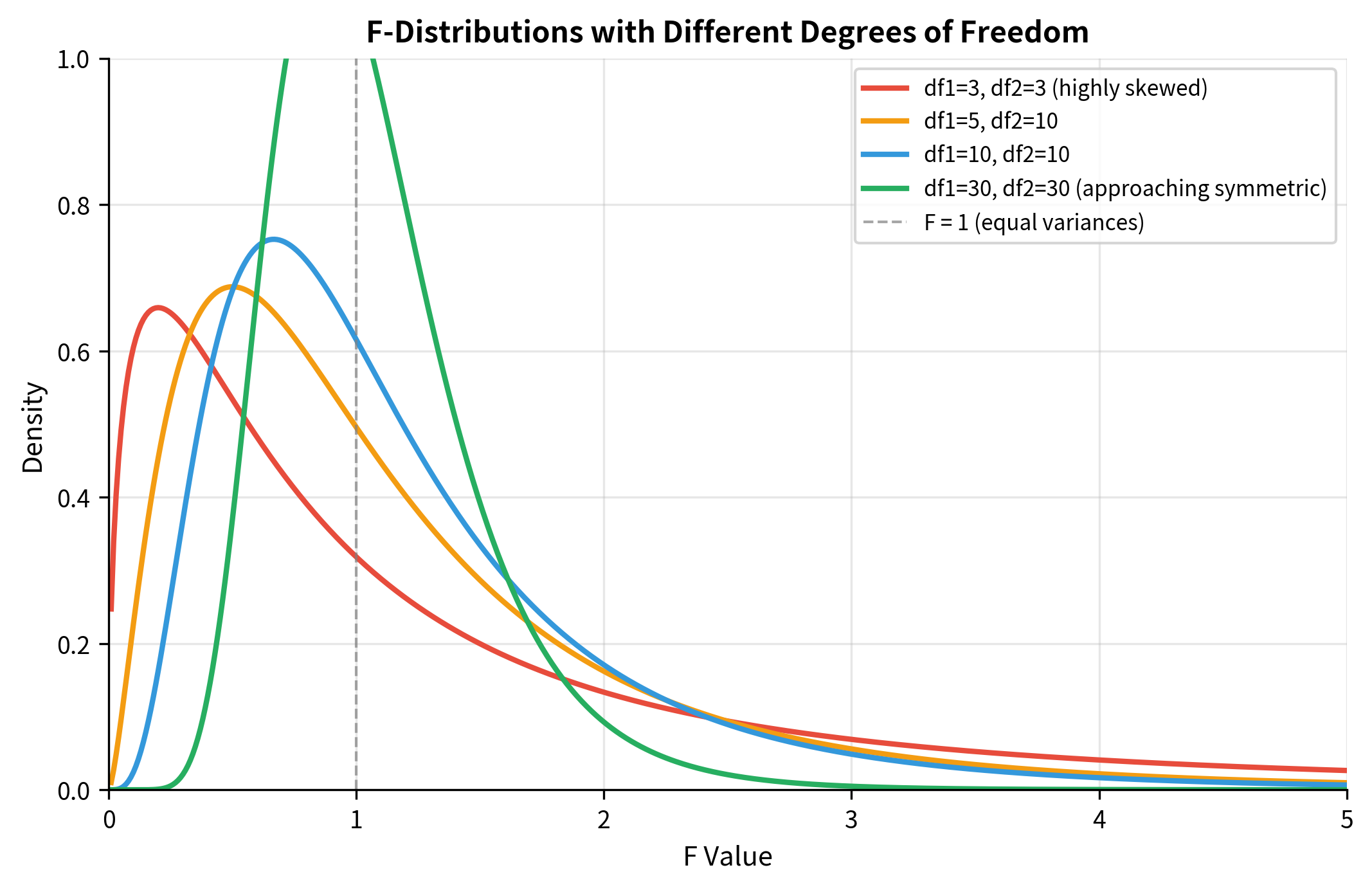
Two degrees of freedom parameters: The F-distribution requires both df1df_1 (numerator) and df2df_2 (denominator). The order matters: F5,10F_{5,10} is a different distribution from F10,5F_{10,5}. This asymmetry reflects the fact that we're comparing a specific numerator variance to a specific denominator variance.

Always non-negative: Since F is a ratio of variances (squared quantities), it cannot be negative. The distribution is defined only for F0F \geq 0.

Right-skewed: The F-distribution has a long right tail, especially when degrees of freedom are small. As both df1df_1 and df2df_2 increase, the distribution becomes more symmetric and concentrated.

Mean near 1 under the null: When comparing equal variances, F should be approximately 1. The expected value is E[F]=df2/(df22)E[F] = df_2/(df_2 - 2) for df2>2df_2 > 2, which approaches 1 as df2df_2 grows large.

Reciprocal relationship: If FFdf1,df2F \sim F_{df_1, df_2}, then 1/FFdf2,df11/F \sim F_{df_2, df_1}. This is useful for two-tailed tests and for ensuring the larger variance is in the numerator.

Out[2]:
Visualization
Line plot showing F-distributions with varying degrees of freedom parameters.
F-distributions with different degrees of freedom. With small df, the distribution is highly right-skewed with a long tail. As degrees of freedom increase, the distribution becomes more concentrated around 1 and more symmetric. The shape depends on both the numerator (df1) and denominator (df2) degrees of freedom.
Out[3]:
Visualization
F-distribution with shaded right-tail rejection region and critical value marked.
The F-distribution with rejection region for a one-tailed test at alpha = 0.05. Since we typically place the larger variance in the numerator, the test rejects when F is in the right tail. The critical value depends on both degrees of freedom.

F-Test for Comparing Two Variances

The most direct application of the F-test compares variances between two independent populations.

Hypotheses and Test Statistic

Null hypothesis: H0:σ12=σ22H_0: \sigma_1^2 = \sigma_2^2 (population variances are equal)

Alternative hypotheses:

  • Two-sided: Ha:σ12σ22H_a: \sigma_1^2 \neq \sigma_2^2
  • One-sided (greater): Ha:σ12>σ22H_a: \sigma_1^2 > \sigma_2^2
  • One-sided (less): Ha:σ12<σ22H_a: \sigma_1^2 < \sigma_2^2

Test statistic:

F=s12s22F = \frac{s_1^2}{s_2^2}

where s12s_1^2 and s22s_2^2 are the sample variances.

Convention: Place the larger sample variance in the numerator so that F1F \geq 1. This simplifies interpretation: if FF is much larger than 1, it suggests the numerator variance is genuinely larger than the denominator variance.

Degrees of freedom: df1=n11df_1 = n_1 - 1 (numerator), df2=n21df_2 = n_2 - 1 (denominator)

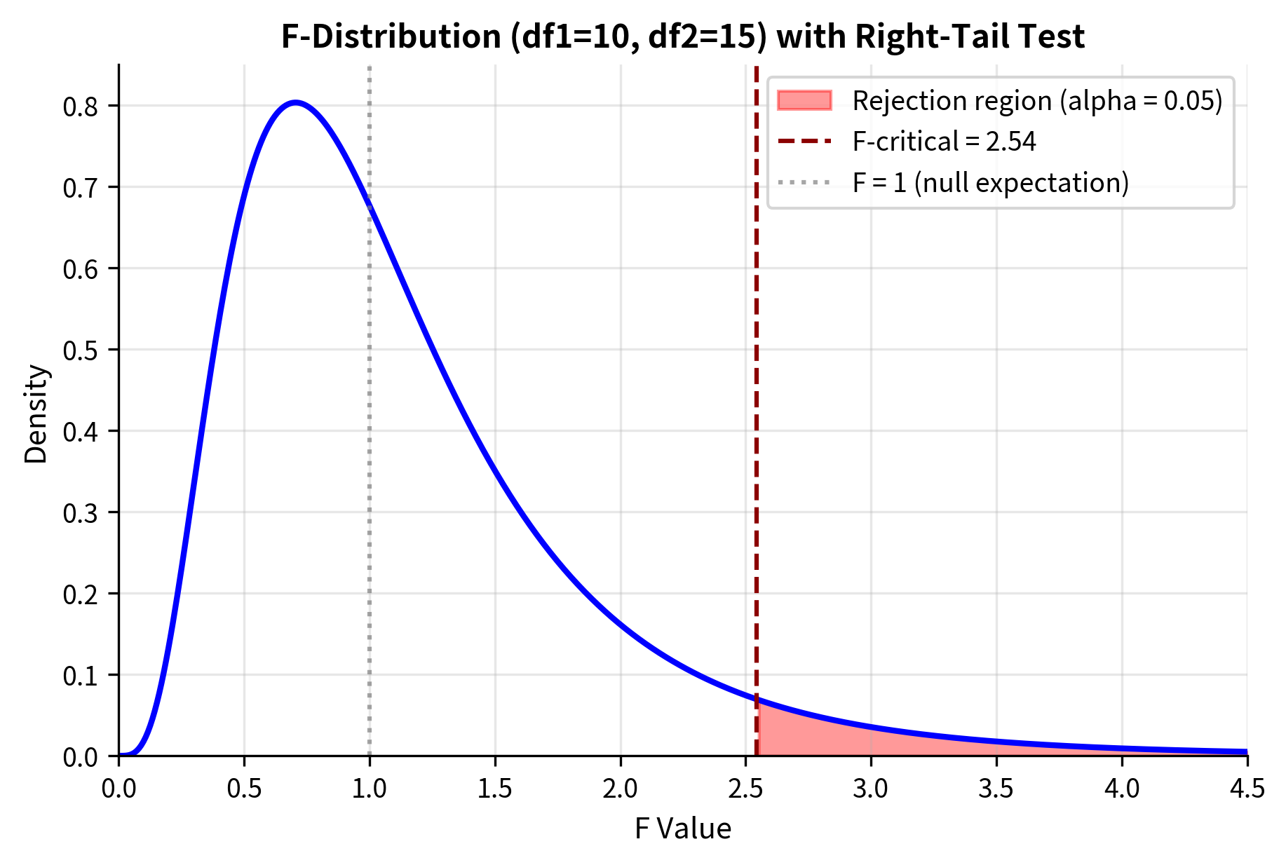
P-value calculation:

  • One-sided (greater): p=P(Fdf1,df2>Fobs)p = P(F_{df_1, df_2} > F_{obs})
  • Two-sided: Since the F-distribution is not symmetric, we compute p=2×min(P(F>Fobs),P(F<Fobs))p = 2 \times \min(P(F > F_{obs}), P(F < F_{obs}))

Worked Example: Manufacturing Process Comparison

A quality engineer wants to compare the consistency of two production lines making precision components. She randomly samples 20 components from Line A and 25 from Line B, measuring a critical dimension.

In[4]:
Code
import numpy as np
from scipy import stats

# Measurements from two production lines (in microns from target)
np.random.seed(42)
line_a = np.random.normal(0, 4.5, 20)  # True std = 4.5 microns
line_b = np.random.normal(0, 7.2, 25)  # True std = 7.2 microns

# Step 1: Calculate sample statistics
n1, n2 = len(line_a), len(line_b)
var1 = np.var(line_a, ddof=1)
var2 = np.var(line_b, ddof=1)
std1, std2 = np.sqrt(var1), np.sqrt(var2)

# Step 2: Arrange so larger variance is in numerator
if var1 >= var2:
    f_stat = var1 / var2
    df1, df2 = n1 - 1, n2 - 1
    larger, smaller = "A", "B"
else:
    f_stat = var2 / var1
    df1, df2 = n2 - 1, n1 - 1
    larger, smaller = "B", "A"

# Step 3: Calculate p-value (two-sided)
p_upper = stats.f.sf(f_stat, df1, df2)
p_value_two_sided = 2 * p_upper  # For two-sided test

# Step 4: Get critical values
f_crit_upper = stats.f.ppf(0.975, df1, df2)
f_crit_lower = stats.f.ppf(0.025, df1, df2)

Let's trace through the calculation:

Step 1: Sample Statistics

sA2=i=120(xixˉ)219,sB2=i=125(xixˉ)224s_A^2 = \frac{\sum_{i=1}^{20}(x_i - \bar{x})^2}{19}, \quad s_B^2 = \frac{\sum_{i=1}^{25}(x_i - \bar{x})^2}{24}

Step 2: F-Statistic

We place the larger variance in the numerator:

F=slarger2ssmaller2F = \frac{s_{larger}^2}{s_{smaller}^2}

Step 3: P-Value

Under H0H_0, this F-statistic follows an Fdf1,df2F_{df_1, df_2} distribution. We find the probability of observing a ratio this extreme.

Out[5]:
Console
F-Test for Comparing Variances: Production Line Comparison
=================================================================

Sample statistics:
-----------------------------------------------------------------
Line A: n = 20, variance = 18.66, std = 4.32 microns
Line B: n = 25, variance = 44.27, std = 6.65 microns

F-test calculation:
-----------------------------------------------------------------
Larger variance (Line B): 44.27
Smaller variance (Line A): 18.66
F-statistic: F = 44.27 / 18.66 = 2.372
Degrees of freedom: df1 = 24, df2 = 19

P-value (two-sided): 0.0588

Critical values (alpha = 0.05, two-sided):
  Lower: 0.426
  Upper: 2.452

Decision (alpha = 0.05):
-----------------------------------------------------------------
Fail to reject H_0: No significant evidence of different variances
Out[6]:
Visualization
Side-by-side boxplots comparing variability of two production lines.
Visual comparison of variability between two production lines. The boxplots show that Line B has greater spread than Line A. The F-test quantifies whether this observed difference is statistically significant or could have occurred by chance.

Important Caveats

The F-test for comparing variances is highly sensitive to non-normality. If the underlying populations are not normally distributed, the F-test can give misleading results even with moderate sample sizes. This is unlike the t-test, which is fairly robust to non-normality.

For this reason, many statisticians prefer more robust alternatives:

  • Levene's test: Uses absolute deviations from the mean or median; robust to non-normality
  • Brown-Forsythe test: A variant of Levene's test using the median
  • Bartlett's test: More powerful under normality but sensitive to non-normality
Practical Recommendation

When checking the equal variance assumption for a t-test:

  1. Visual inspection (boxplots, standard deviation ratio) is often sufficient
  2. If a formal test is needed, use Levene's test rather than the F-test
  3. When in doubt about equal variances, simply use Welch's t-test, which doesn't assume equal variances
In[7]:
Code
from scipy import stats

# Comparing F-test vs Levene's test
np.random.seed(42)
group1 = np.random.normal(50, 5, 30)
group2 = np.random.normal(50, 10, 30)

# F-test
f_stat = np.var(group2, ddof=1) / np.var(group1, ddof=1)
f_pvalue = 2 * stats.f.sf(f_stat, 29, 29)

# Levene's test (more robust)
levene_stat, levene_pvalue = stats.levene(group1, group2)

print("Comparison of variance equality tests:")
print("-" * 50)
print(f"F-test:      F = {f_stat:.2f}, p = {f_pvalue:.4f}")
print(f"Levene's:    W = {levene_stat:.2f}, p = {levene_pvalue:.4f}")
print()
print("Both detect the variance difference, but Levene's test")
print("is preferred because it's robust to non-normality.")
Out[7]:
Console
Comparison of variance equality tests:
--------------------------------------------------
F-test:      F = 4.28, p = 0.0002
Levene's:    W = 14.64, p = 0.0003

Both detect the variance difference, but Levene's test
is preferred because it's robust to non-normality.

F-Test in Regression: Overall Model Significance

Beyond comparing two variances, the F-test plays a central role in regression analysis. When you fit a regression model, an immediate question is: does this model explain any variation at all?

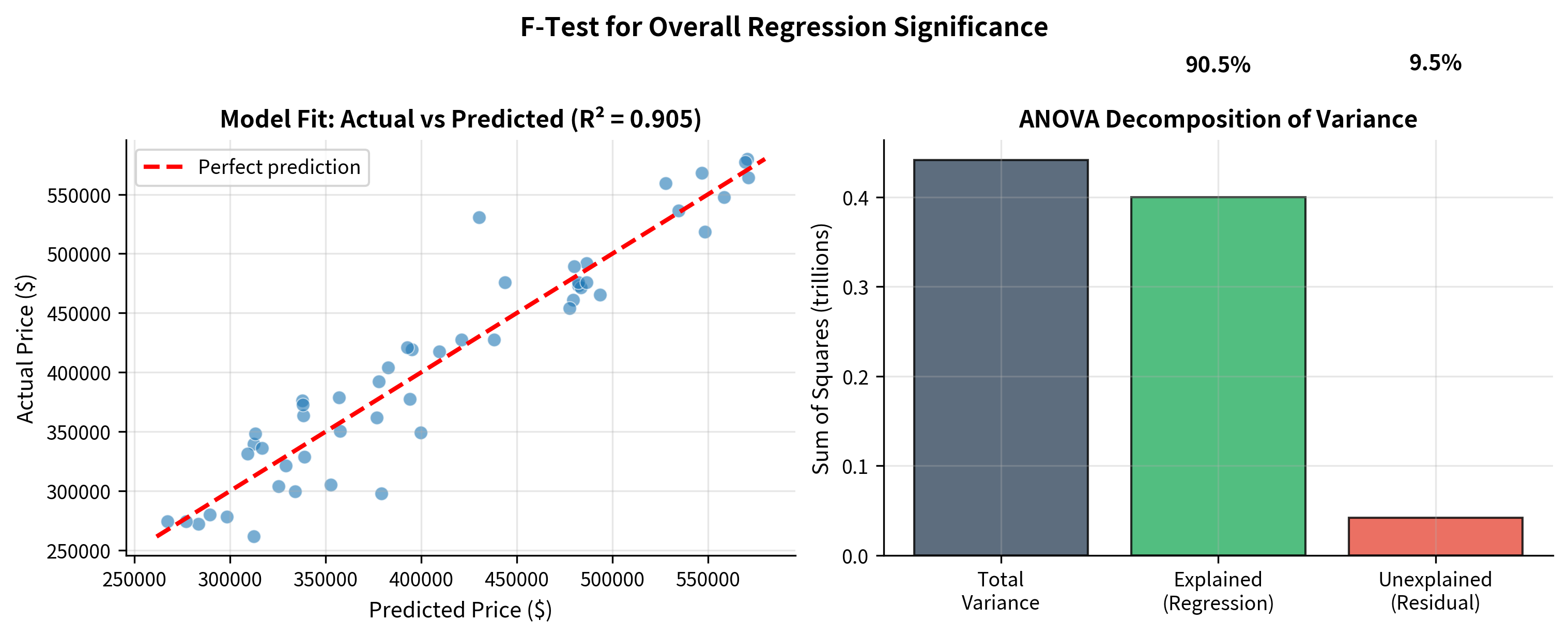
The ANOVA Decomposition

Every regression model partitions the total variation in the response variable into two components:

SSTotal=SSRegression+SSResidualSS_{Total} = SS_{Regression} + SS_{Residual}

where:

  • SSTotalSS_{Total} = i=1n(yiyˉ)2\sum_{i=1}^{n}(y_i - \bar{y})^2 : Total variation in yy
  • SSRegressionSS_{Regression} = i=1n(y^iyˉ)2\sum_{i=1}^{n}(\hat{y}_i - \bar{y})^2 : Variation explained by the model
  • SSResidualSS_{Residual} = i=1n(yiy^i)2\sum_{i=1}^{n}(y_i - \hat{y}_i)^2 : Variation left unexplained

The F-test asks: is the explained variation large enough, relative to the unexplained variation, to conclude that the model has real predictive value?

The F-Statistic for Regression

Test statistic:

F=SSRegression/pSSResidual/(np1)=MSRegressionMSResidualF = \frac{SS_{Regression} / p}{SS_{Residual} / (n - p - 1)} = \frac{MS_{Regression}}{MS_{Residual}}

where:

  • pp = number of predictors (excluding intercept)
  • nn = number of observations
  • MSMS = "Mean Square" = sum of squares divided by degrees of freedom

Degrees of freedom:

  • Numerator: df1=pdf_1 = p (one for each predictor)
  • Denominator: df2=np1df_2 = n - p - 1 (residual degrees of freedom)

Null hypothesis: H0:β1=β2==βp=0H_0: \beta_1 = \beta_2 = \cdots = \beta_p = 0 (all predictor coefficients are zero)

If the null is true, none of the predictors help explain yy, and MSRegressionMS_{Regression} should be similar to MSResidualMS_{Residual}, giving F1F \approx 1. A large F indicates the model explains more variation than expected by chance.

Worked Example: Multiple Regression

A researcher studies factors affecting house prices, fitting a model with square footage and number of bedrooms as predictors.

In[8]:
Code
import numpy as np
from scipy import stats

# Generate housing data
np.random.seed(42)
n = 50

sqft = np.random.uniform(1000, 3000, n)
bedrooms = np.random.randint(2, 6, n)
price = 50000 + 150 * sqft + 20000 * bedrooms + np.random.normal(0, 30000, n)

# Fit regression using linear algebra
X = np.column_stack([np.ones(n), sqft, bedrooms])
beta = np.linalg.lstsq(X, price, rcond=None)[0]
y_pred = X @ beta

# Calculate sums of squares
y_bar = np.mean(price)
ss_total = np.sum((price - y_bar) ** 2)
ss_residual = np.sum((price - y_pred) ** 2)
ss_regression = ss_total - ss_residual

# Degrees of freedom
p = 2  # number of predictors (sqft and bedrooms)
df_regression = p
df_residual = n - p - 1
df_total = n - 1

# Mean squares
ms_regression = ss_regression / df_regression
ms_residual = ss_residual / df_residual

# F-statistic and p-value
f_stat = ms_regression / ms_residual
p_value = stats.f.sf(f_stat, df_regression, df_residual)

# R-squared
r_squared = ss_regression / ss_total
adj_r_squared = 1 - (1 - r_squared) * (n - 1) / (n - p - 1)
Out[9]:
Console
F-Test for Regression: House Price Model
=================================================================

Model: Price = beta_0 + beta_1 * SquareFootage + beta_2 * Bedrooms + epsilon

Fitted coefficients:
  Intercept (beta_0):     $64,173
  Square footage (beta_1): $147.43 per sqft
  Bedrooms (beta_2):       $18,284 per bedroom

ANOVA Table:
-----------------------------------------------------------------
Source                   SS     df             MS          F            p
-----------------------------------------------------------------
Regression   399,645,915,189      2 199,822,957,594     224.36     9.04e-25
Residual     41,860,284,034     47    890,644,341
Total        441,506,199,223     49
-----------------------------------------------------------------

R-squared:          0.9052
Adjusted R-squared: 0.9012

Interpretation: The model explains 90.5% of the variance in house prices.
The F-test (F = 224.4, p < 0.001) confirms this is statistically significant.
Out[10]:
Visualization
Two-panel figure showing regression fit and variance decomposition.
Visualization of regression model fit and the variance decomposition. The left panel shows actual vs. predicted house prices, demonstrating the model's explanatory power. The right panel shows the ANOVA decomposition of total variance into explained (regression) and unexplained (residual) components.

Connection to R-Squared

The F-statistic is directly related to R2R^2:

F=R2/p(1R2)/(np1)F = \frac{R^2 / p}{(1 - R^2) / (n - p - 1)}

This shows that:

  • Higher R2R^2 → larger F → smaller p-value
  • More predictors (pp) → penalizes the F-statistic (need more explained variance to be significant)
  • Larger sample size (nn) → more power to detect small R2R^2 as significant

Comparing Nested Models

One of the most powerful applications of the F-test is comparing nested regression models. A model is "nested" within another if it's a special case obtained by setting some coefficients to zero.

Question: Does adding extra predictors significantly improve the model?

The Nested Model F-Test

Consider:

  • Reduced model: y=β0+β1x1+ϵy = \beta_0 + \beta_1 x_1 + \epsilon (1 predictor)
  • Full model: y=β0+β1x1+β2x2+β3x3+ϵy = \beta_0 + \beta_1 x_1 + \beta_2 x_2 + \beta_3 x_3 + \epsilon (3 predictors)

The reduced model is nested within the full model (set β2=β3=0\beta_2 = \beta_3 = 0).

Test statistic:

F=(SSres,reducedSSres,full)/(dfreduceddffull)SSres,full/dffullF = \frac{(SS_{res,reduced} - SS_{res,full}) / (df_{reduced} - df_{full})}{SS_{res,full} / df_{full}}

Interpretation:

  • Numerator: Improvement (reduction in residual SS) per additional predictor
  • Denominator: Unexplained variance per degree of freedom in the full model
  • dfreduceddffulldf_{reduced} - df_{full} = number of additional predictors being tested

Null hypothesis: The additional predictors have no effect (β2=β3=0\beta_2 = \beta_3 = 0)

Worked Example: Model Selection

A researcher wants to know if adding interaction terms improves a base model.

In[11]:
Code
import numpy as np
from scipy import stats


def compare_nested_models(y, X_reduced, X_full):
    """
    Compare nested regression models using F-test.

    Returns F-statistic, p-value, and improvement in R-squared.
    """
    n = len(y)

    # Fit both models
    beta_reduced = np.linalg.lstsq(X_reduced, y, rcond=None)[0]
    beta_full = np.linalg.lstsq(X_full, y, rcond=None)[0]

    y_pred_reduced = X_reduced @ beta_reduced
    y_pred_full = X_full @ beta_full

    # Residual sums of squares
    ss_res_reduced = np.sum((y - y_pred_reduced) ** 2)
    ss_res_full = np.sum((y - y_pred_full) ** 2)
    ss_total = np.sum((y - np.mean(y)) ** 2)

    # R-squared for each model
    r2_reduced = 1 - ss_res_reduced / ss_total
    r2_full = 1 - ss_res_full / ss_total

    # Degrees of freedom
    p_reduced = X_reduced.shape[1] - 1
    p_full = X_full.shape[1] - 1

    df_reduced = n - p_reduced - 1
    df_full = n - p_full - 1
    df_diff = df_reduced - df_full  # = number of added predictors

    # F-statistic
    f_stat = ((ss_res_reduced - ss_res_full) / df_diff) / (
        ss_res_full / df_full
    )
    p_value = stats.f.sf(f_stat, df_diff, df_full)

    return {
        "f_stat": f_stat,
        "df_num": df_diff,
        "df_denom": df_full,
        "p_value": p_value,
        "r2_reduced": r2_reduced,
        "r2_full": r2_full,
        "r2_change": r2_full - r2_reduced,
    }


# Example: Testing whether x2 and interaction add value
np.random.seed(42)
n = 60
x1 = np.random.normal(0, 1, n)
x2 = np.random.normal(0, 1, n)
x3_noise = np.random.normal(0, 1, n)  # Pure noise

# True model: y depends on x1 and x2, with interaction
y = 5 + 3 * x1 + 2 * x2 + 1.5 * x1 * x2 + np.random.normal(0, 1, n)

# Define nested models
X_base = np.column_stack([np.ones(n), x1])
X_with_x2 = np.column_stack([np.ones(n), x1, x2])
X_full = np.column_stack([np.ones(n), x1, x2, x1 * x2])
X_with_noise = np.column_stack([np.ones(n), x1, x2, x1 * x2, x3_noise])

# Compare models
result1 = compare_nested_models(y, X_base, X_with_x2)
result2 = compare_nested_models(y, X_with_x2, X_full)
result3 = compare_nested_models(y, X_full, X_with_noise)
Out[12]:
Console
Nested Model Comparisons Using F-Test
======================================================================

True model: y = 5 + 3*x1 + 2*x2 + 1.5*x1*x2 + noise

Comparison 1: Base model (x1 only) vs. adding x2
----------------------------------------------------------------------
  R² change:   0.6016 -> 0.7688 (+0.1672)
  F(1, 57) = 41.22, p = 2.93e-08
  Conclusion:  Adding x2 significantly improves model

Comparison 2: Model with x1, x2 vs. adding interaction x1*x2
----------------------------------------------------------------------
  R² change:   0.7688 -> 0.9221 (+0.1534)
  F(1, 56) = 110.26, p = 7.56e-15
  Conclusion:  Adding interaction significantly improves model

Comparison 3: Full model vs. adding noise variable x3
----------------------------------------------------------------------
  R² change:   0.9221 -> 0.9222 (+0.0001)
  F(1, 55) = 0.08, p = 0.7776
  Conclusion:  x3 (noise) does not improve model, as expected

The F-test correctly identifies:

  1. Adding x2x_2 (true predictor) significantly improves the model
  2. Adding the interaction x1x2x_1 \cdot x_2 (true effect) significantly improves the model
  3. Adding x3x_3 (pure noise) does not significantly improve the model

When to Use Nested Model Comparison

This technique is useful for:

  • Variable selection: Testing whether specific predictors should be included
  • Testing interactions: Does an interaction term add explanatory power?
  • Polynomial terms: Does a quadratic term improve on a linear model?
  • Group comparisons: Testing whether different groups need different slopes (via interaction with a group indicator)

Assumptions and Limitations

Assumptions of F-Tests

1. Independence: Observations must be independent within and between groups

2. Normality: The underlying populations should be normally distributed

  • The F-test for variances is highly sensitive to non-normality
  • The regression F-test is more robust, especially with larger samples

3. Random sampling: Data should come from random samples of the populations of interest

Robustness Considerations

ApplicationRobustness to Non-Normality
Comparing two variancesPoor - Use Levene's test instead
Overall regression significanceModerate - OK with n > 30
Nested model comparisonModerate - OK with larger samples
ANOVA (covered next)Moderate - OK if groups have similar sizes

Summary

The F-test and F-distribution are fundamental tools for comparing variances and testing model adequacy:

The F-distribution:

  • Arises from the ratio of two independent variance estimates
  • Parameterized by two degrees of freedom (numerator and denominator)
  • Always non-negative, right-skewed, centered near 1 under the null hypothesis
  • Converges to symmetry as degrees of freedom increase

F-test for comparing variances:

  • Tests H0:σ12=σ22H_0: \sigma_1^2 = \sigma_2^2
  • Statistic: F=s12/s22F = s_1^2 / s_2^2 (larger variance in numerator)
  • Sensitive to non-normality; prefer Levene's test in practice

F-test in regression:

  • Overall significance: Tests whether any predictors have explanatory power
  • Decomposes total variance into explained and unexplained components
  • Large F indicates model explains more variation than expected by chance

Nested model comparison:

  • Tests whether additional predictors significantly improve a model
  • Compares reduction in residual variance to residual variance of full model
  • Essential for variable selection and model building

Practical guidance:

  • For comparing variances: Use Levene's test (more robust) or visual inspection
  • For regression: The F-test from standard output tests overall model significance
  • For model selection: Nested model F-tests guide inclusion of predictors

What's Next

This chapter introduced the F-distribution and F-tests for comparing variances and testing regression models. The next chapter on ANOVA (Analysis of Variance) shows how the F-test extends to comparing means across three or more groups. ANOVA uses the same variance decomposition logic: partition total variation into between-group and within-group components, then test whether between-group variation is large enough to conclude the means differ.

After ANOVA, subsequent chapters cover:

All of these build on the foundation of understanding how variation is partitioned and compared, which you've learned through z-tests, t-tests, and now F-tests.

Quiz

Ready to test your understanding? Take this quick quiz to reinforce what you've learned about the F-test and F-distribution.

Loading component...

Reference

BIBTEXAcademic
@misc{theftestandfdistributioncomparingvariancesregressionnestedmodels, author = {Michael Brenndoerfer}, title = {The F-Test and F-Distribution: Comparing Variances, Regression & Nested Models}, year = {2026}, url = {https://mbrenndoerfer.com/writing/f-test-f-distribution-comparing-variances-regression-nested-models}, organization = {mbrenndoerfer.com}, note = {Accessed: 2025-01-01} }
APAAcademic
Michael Brenndoerfer (2026). The F-Test and F-Distribution: Comparing Variances, Regression & Nested Models. Retrieved from https://mbrenndoerfer.com/writing/f-test-f-distribution-comparing-variances-regression-nested-models
MLAAcademic
Michael Brenndoerfer. "The F-Test and F-Distribution: Comparing Variances, Regression & Nested Models." 2026. Web. today. <https://mbrenndoerfer.com/writing/f-test-f-distribution-comparing-variances-regression-nested-models>.
CHICAGOAcademic
Michael Brenndoerfer. "The F-Test and F-Distribution: Comparing Variances, Regression & Nested Models." Accessed today. https://mbrenndoerfer.com/writing/f-test-f-distribution-comparing-variances-regression-nested-models.
HARVARDAcademic
Michael Brenndoerfer (2026) 'The F-Test and F-Distribution: Comparing Variances, Regression & Nested Models'. Available at: https://mbrenndoerfer.com/writing/f-test-f-distribution-comparing-variances-regression-nested-models (Accessed: today).
SimpleBasic
Michael Brenndoerfer (2026). The F-Test and F-Distribution: Comparing Variances, Regression & Nested Models. https://mbrenndoerfer.com/writing/f-test-f-distribution-comparing-variances-regression-nested-models