

A comprehensive guide to CART (Classification and Regression Trees), including mathematical foundations, Gini impurity, variance reduction, and practical implementation with scikit-learn. Learn how to build interpretable decision trees for both classification and regression tasks.

This article is part of the free-to-read Machine Learning from Scratch
Choose your expertise level to adjust how many terms are explained. Beginners see more tooltips, experts see fewer to maintain reading flow. Hover over underlined terms for instant definitions.
CART (Classification and Regression Trees)
CART, or Classification and Regression Trees, represents one of the most intuitive and interpretable machine learning algorithms. At its core, CART builds decision trees by recursively partitioning the feature space into regions that best separate the target variable. Think of it as creating a flowchart where each decision point asks a simple yes/no question about a feature, ultimately leading to a prediction.
CART's simplicity and transparency make it particularly valuable in domains where interpretability is crucial, such as healthcare, finance, and regulatory compliance. Unlike black-box algorithms, every decision made by a CART model can be traced back to specific feature thresholds and logical rules. The algorithm works by finding the optimal splits that minimize impurity (for classification) or variance (for regression) at each node.
CART differs from other tree-based methods in several key ways. Unlike ensemble methods like Random Forest or Gradient Boosting that we will cover later, CART builds a single tree without any randomization or boosting mechanisms. It also uses a greedy approach, making the locally optimal split at each node without considering the global impact on the final tree structure. This can sometimes lead to suboptimal trees, but it makes the algorithm computationally efficient and easy to understand.
CART uses a greedy algorithm, meaning it makes the best decision at each step without considering future consequences. At each node, it chooses the split that provides the maximum immediate reduction in impurity, even if this might not lead to the globally optimal tree structure. This is similar to a chess player who always makes the best move for the current position without planning several moves ahead. While this approach is computationally efficient, it can sometimes result in trees that are not globally optimal.
The algorithm's recursive nature means it continues splitting until it reaches a stopping criterion, such as maximum depth, minimum samples per leaf, or when no further improvement can be made. This process creates a hierarchical structure where each path from root to leaf represents a unique decision rule that can be easily translated into human-readable if-then statements.
Advantages
CART models offer exceptional interpretability that sets them apart from many other algorithms. Unlike neural networks or ensemble methods, every prediction can be traced through a clear sequence of if-then rules. This makes CART particularly valuable in regulated industries like healthcare and finance, where model decisions must be explainable to auditors, regulators, and end users. A doctor can follow the tree path to understand why a patient was classified as high-risk, making CART well-suited for clinical decision support systems.
The algorithm handles real-world data problems gracefully, demonstrating remarkable robustness to data quality issues. It can work with datasets containing missing values, outliers, and mixed data types without extensive preprocessing. The algorithm's use of surrogate splits means that even when primary features are missing, alternative decision paths can still provide reasonable predictions. This robustness makes CART particularly valuable for exploratory data analysis and rapid prototyping scenarios where data quality may be uncertain.
CART naturally captures complex interactions between features without requiring manual feature engineering, effectively performing automatic feature engineering during the tree-building process. The algorithm can discover non-obvious relationships, such as "if age > 65 AND income < 30k AND has_diabetes = true, then high_risk = true." These discovered patterns often provide valuable business insights beyond just predictions, making CART useful for both modeling and data exploration purposes.
Training and prediction with CART are computationally efficient, providing significant performance advantages. The greedy splitting approach, while sometimes suboptimal, ensures that training time scales reasonably with data size. This efficiency makes CART well-suited for embedded systems, mobile applications, and scenarios requiring low-latency predictions where computational resources are constrained.
Disadvantages
CART models exhibit high variance, meaning small changes in training data can produce substantially different trees. This instability stems from the algorithm's sensitivity to data variations and its tendency to overfit. A single outlier or mislabeled sample can significantly alter the tree structure, which can be problematic for applications where consistency is important. This high variance also means that cross-validation results can vary between runs, making it challenging to obtain stable performance estimates.
The algorithm struggles with simple linear relationships that other algorithms handle effortlessly. While a linear regression can capture a relationship like "price = 2 × size + 100" with a single equation, CART might need dozens of splits to approximate the same relationship. This inefficiency makes CART suboptimal for problems where linear relationships dominate, such as many economic and physical modeling scenarios where the underlying relationships are inherently linear.
The algorithm exhibits a strong bias toward features with high cardinality or many unique values. Categorical features with many categories (like ZIP codes or product IDs) and continuous features with many distinct values get unfairly favored during split selection. This bias can lead to trees that perform well on training data but generalize poorly, as they may be overfitting to spurious patterns in high-cardinality features rather than learning meaningful relationships.
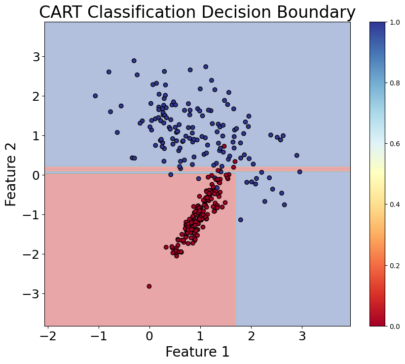
While CART can capture interactions, it's constrained by its axis-parallel splits, limiting its expressiveness for complex geometric patterns. It cannot efficiently represent certain geometric patterns, such as diagonal decision boundaries or circular regions, that might be natural for the underlying data. This limitation becomes particularly problematic in high-dimensional spaces where the curse of dimensionality makes axis-parallel splits increasingly ineffective at capturing the true data structure.
CART can only create axis-parallel splits, meaning it can only split along lines that are parallel to the feature axes. This means it cannot create diagonal or curved decision boundaries. For example, if the optimal decision boundary is a diagonal line (like ), CART will need many small rectangular regions to approximate this boundary, leading to a complex tree structure. This is why other algorithms like Support Vector Machines or Neural Networks might be more appropriate for problems with complex geometric patterns.
Standard decision trees, including CART, cannot extrapolate to unseen ranges of input features. Unlike linear models that can extend predictions beyond the training data range, decision trees are constrained to make predictions only within the feature ranges observed during training.
For example, if a tree was trained on house prices for properties between 1,000-3,000 square feet, it cannot make reliable predictions for a 5,000 square foot house. The tree will simply use the prediction from the leaf node corresponding to the highest training value (3,000+ square feet), which may be completely inappropriate for the new, larger property. This limitation is particularly problematic in time series forecasting, growth modeling, and any scenario where you need to predict beyond the observed data range.
Formula - Classification
The mathematical foundation of CART revolves around finding the optimal split that minimizes impurity for classification or variance for regression. Let's walk through these concepts step by step.
Gini Impurity
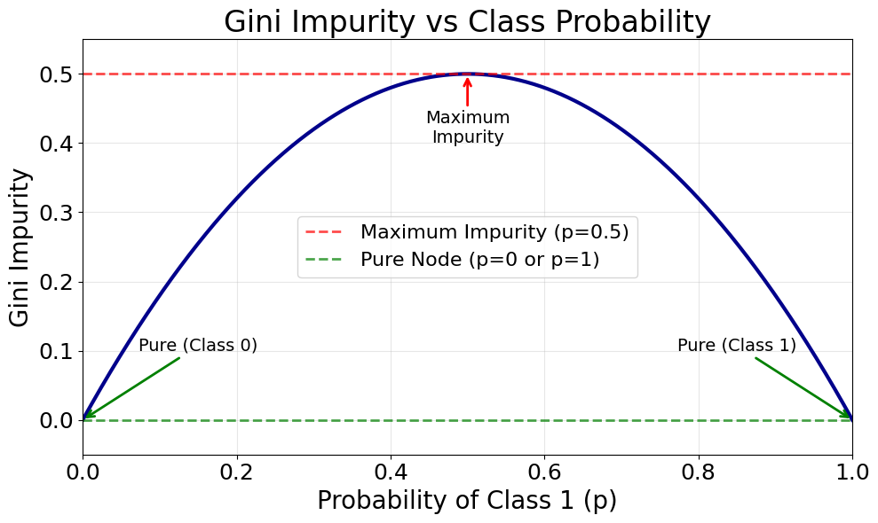
For classification problems, CART uses the Gini impurity measure to evaluate the quality of a split. The Gini impurity measures how often a randomly chosen element would be incorrectly labeled if it were randomly labeled according to the distribution of labels in the subset.
We start with the basic Gini impurity formula for a node:
where:
- is the Gini impurity for node (a measure of impurity ranging from 0 for pure nodes to a maximum value when classes are evenly distributed)
- represents the set of samples at the current node (the subset of training data that reaches this node)
- is the number of classes (total number of distinct class labels in the classification problem)
- is the proportion of samples belonging to class in the set (calculated as where is the number of samples of class and is the total number of samples in node )
- is the class index (ranging from 1 to )
The reason we square the probabilities is to penalize nodes where the class distribution is mixed. When all samples belong to the same class (complete purity), for one class and for all others, making . When classes are evenly distributed, the Gini impurity reaches its maximum.
To find the best split, we calculate the weighted average of the Gini impurities of the resulting child nodes:
where:
- is the weighted Gini impurity after splitting node (the combined impurity of both child nodes, weighted by their sizes)
- is the left child node after the split (the subset of samples that satisfy the split condition)
- is the right child node after the split (the subset of samples that do not satisfy the split condition)
- is the number of samples in the parent node (total samples before splitting)
- is the number of samples in the left child node (samples satisfying the split condition)
- is the number of samples in the right child node (samples not satisfying the split condition, where )
- and are the weights (proportions of samples going to each child node, ensuring larger child nodes have more influence on the overall impurity measure)
The algorithm selects the split that minimizes this weighted Gini impurity. This makes intuitive sense: we want splits that create child nodes with as pure class distributions as possible.
Regression: Mean Squared Error
For regression problems, CART minimizes the variance (or equivalently, the mean squared error) of the target variable within each leaf node. The variance for a node is calculated as:
where:
- is the variance of the target variable in node (a measure of how spread out the target values are around their mean)
- is the number of samples in node (total count of data points in this node)
- is the target value for sample (the actual observed response value for the -th sample in node )
- is the mean target value in the node (the average of all target values in node )
- indicates summation over all samples in node
The mean target value is calculated as:
where:
- is the mean target value (the arithmetic average of all target values in node , which becomes the prediction for this node)
- is the normalization factor (ensures we compute the average rather than the sum)
- is the sum of all target values in node
The mean squared error is essentially the same as variance, just without the division by :
where:
- is the mean squared error for node (the sum of squared deviations from the mean, used as an alternative to variance)
- is the squared deviation of sample from the mean (measures how far each sample's target value is from the node's average)
For a split, we calculate the weighted sum of the MSEs of the child nodes:
where:
- is the total mean squared error after splitting node (the sum of MSEs from both child nodes)
- is the mean squared error of the left child node (calculated as )
- is the mean squared error of the right child node (calculated as )
This is equivalent to the weighted variance approach used in classification, but since we're dealing with continuous values, we use the sum of squared deviations from the mean.
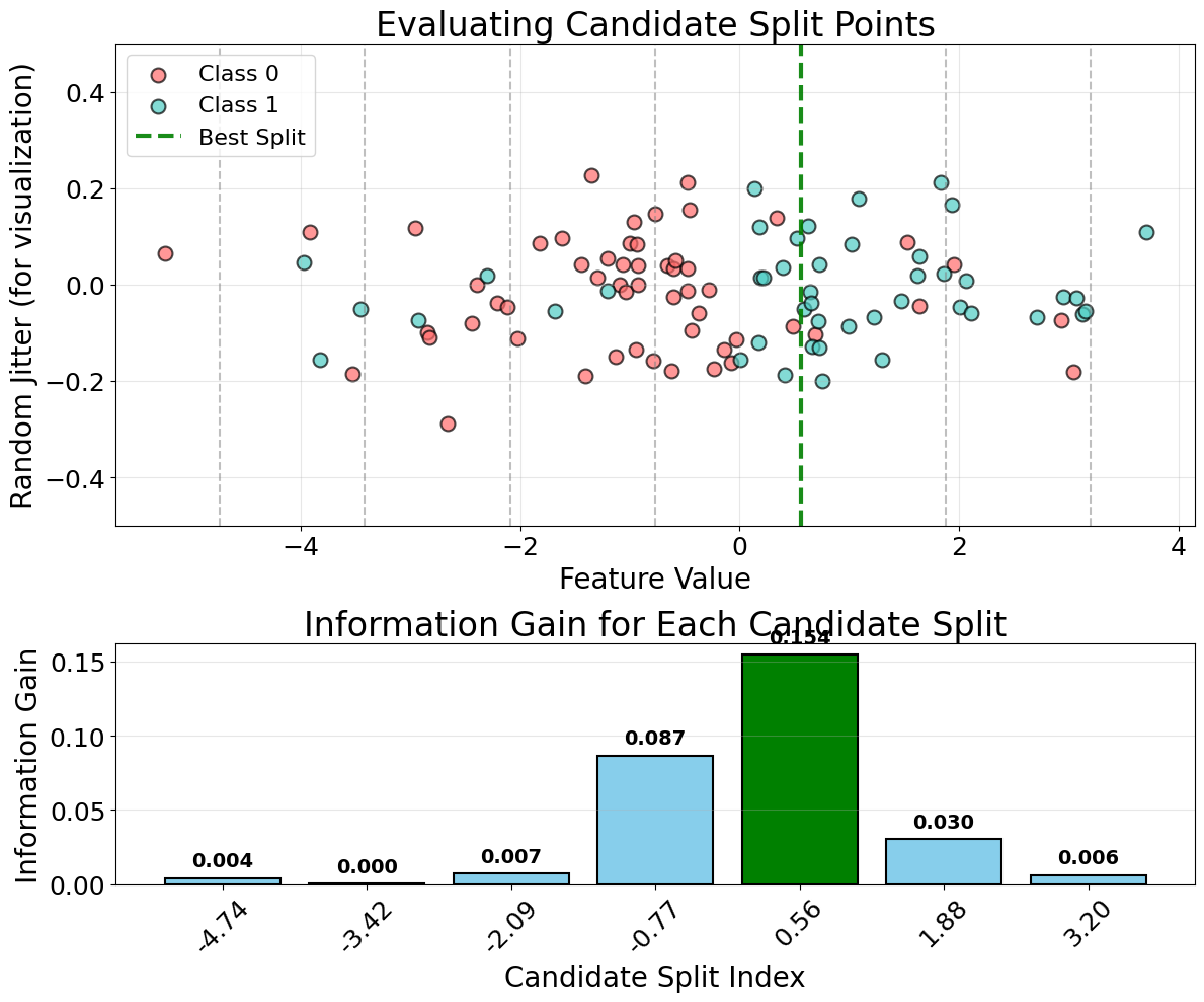
Split Selection Process
The algorithm evaluates all possible splits for each feature and selects the one that provides the maximum reduction in impurity or variance. For a continuous feature with values , we consider splits of the form for all possible thresholds . For categorical features, we consider all possible subsets of categories.
The information gain (or variance reduction) for a split is:
where:
- is the information gain (the reduction in impurity achieved by the split, with higher values indicating better splits)
- is the impurity of the parent node before splitting (either Gini impurity for classification or variance for regression)
- is the weighted impurity after splitting (the combined impurity of both child nodes)
For classification, this becomes:
where:
- is the Gini impurity of the parent node before splitting
- is the weighted Gini impurity after splitting (calculated as )
For regression, this becomes:
where:
- is the variance of the parent node before splitting
- is the weighted variance of the left child node
- is the weighted variance of the right child node
The algorithm selects the split with the maximum gain, ensuring that each split provides the most significant improvement in model performance.
Mathematical Properties
The Gini impurity and variance measures are monotonically decreasing as we make better splits. This property ensures that the algorithm chooses splits that improve the overall model quality.
The impurity functions are convex, meaning that the weighted average of impurities from child nodes is less than or equal to the parent node's impurity. This ensures that splitting does not increase the overall impurity.
For each feature, the algorithm must evaluate all possible split points. For continuous features with unique values, this requires evaluations. For categorical features with categories, it requires evaluating possible splits, making it computationally expensive for high-cardinality categorical features.
where:
- is the number of unique values for a continuous feature (the distinct values that could serve as split thresholds)
- represents linear computational complexity (evaluating each unique value as a potential split point)
- is the number of categories for a categorical feature (the distinct category labels)
- is the number of possible binary partitions of categories (exponential growth with the number of categories)
The computational complexity of CART grows significantly with the number of features and their cardinality. For a dataset with features and samples, the worst-case time complexity is for continuous features, but can be much higher for categorical features with many categories.
where:
- is the number of features (predictor variables in the dataset)
- is the number of samples (data points in the training set)
- represents the computational complexity (the algorithm must evaluate features, and for each feature with samples, sorting takes time)
This is why preprocessing steps like feature selection or categorical encoding are often necessary for large-scale applications.
Formula - Regression
The mathematical foundation of CART for regression problems focuses on minimizing variance (or equivalently, mean squared error) at each split. Unlike classification, where we measure impurity, regression trees aim to create leaf nodes with the lowest possible variance in the target variable.
Mean Squared Error
For regression problems, CART uses the mean squared error (MSE) to evaluate the quality of a split. The MSE measures the average squared difference between the predicted values and the actual target values in a node.
We start with the basic MSE formula for a node:
where:
- is the mean squared error for node (the average squared deviation of target values from their mean)
- is the number of samples in node (total count of data points in this node)
- is the target value for sample (the actual observed response value for the -th sample in node )
- is the mean target value in the node (the average of all target values in node )
- indicates summation over all samples in node
The mean target value is calculated as:
where:
- is the mean target value (the arithmetic average of all target values in node , which becomes the prediction for this node)
- is the normalization factor (ensures we compute the average rather than the sum)
- is the sum of all target values in node
The reason we use squared differences is to penalize larger errors more heavily than smaller ones. This ensures that the algorithm prioritizes splits that create more homogeneous groups in terms of their target values. When all samples in a node have the same target value (complete homogeneity), the MSE equals zero.
To find the best split, we calculate the weighted sum of the MSEs of the resulting child nodes:
where:
- is the weighted mean squared error after splitting node (the combined MSE of both child nodes, weighted by their sizes)
- is the left child node after the split (the subset of samples that satisfy the split condition)
- is the right child node after the split (the subset of samples that do not satisfy the split condition)
- is the number of samples in the parent node (total samples before splitting)
- is the number of samples in the left child node (samples satisfying the split condition)
- is the number of samples in the right child node (samples not satisfying the split condition, where )
- and are the weights (proportions of samples going to each child node, ensuring larger child nodes have more influence on the overall MSE measure)
The algorithm selects the split that minimizes this weighted MSE. This makes intuitive sense: we want splits that create child nodes with as low variance as possible in their target values.
Variance Reduction
An alternative and equivalent approach is to use variance instead of MSE. The variance for a node is calculated as:
where:
- is the variance of the target variable in node (identical to MSE, measuring spread of target values)
- All other symbols have the same meaning as in the MSE formula above
For a split, we calculate the weighted sum of the variances of the child nodes:
where:
- is the weighted variance after splitting node (the combined variance of both child nodes, weighted by their sizes)
- is the variance of the left child node (calculated as )
- is the variance of the right child node (calculated as )
- All other symbols have the same meaning as defined previously
The variance reduction for a split is:
where:
- is the reduction in variance achieved by the split (the decrease in variance from parent to weighted child nodes, with higher values indicating better splits)
- is the variance of the parent node before splitting
- is the weighted variance after splitting
The algorithm selects the split that provides the maximum variance reduction, which is equivalent to minimizing the weighted MSE.
Split Selection Process
The algorithm evaluates all possible splits for each feature and selects the one that provides the maximum variance reduction. For a continuous feature with values , we consider splits of the form for all possible thresholds . For categorical features, we consider all possible subsets of categories.
The information gain (or variance reduction) for a split is:
where:
- is the variance reduction (the decrease in variance achieved by the split, with higher values indicating better splits)
- is the variance of the parent node before splitting
- is the weighted variance contribution of the left child node
- is the weighted variance contribution of the right child node
- The right-hand side can be rewritten as , showing this is equivalent to the variance reduction formula above
The algorithm selects the split with the maximum gain, ensuring that each split provides the most significant reduction in variance.
Mathematical Properties
The MSE and variance measures are monotonically decreasing as we make better splits. This property ensures that the algorithm chooses splits that improve the overall model quality.
The variance functions are convex, meaning that the weighted average of variances from child nodes is less than or equal to the parent node's variance. This ensures that splitting does not increase the overall variance.
For each feature, the algorithm must evaluate all possible split points. For continuous features with unique values, this requires evaluations. For categorical features with categories, it requires evaluating possible splits, making it computationally expensive for high-cardinality categorical features.
where:
- is the number of unique values for a continuous feature (the distinct values that could serve as split thresholds)
- represents linear computational complexity (evaluating each unique value as a potential split point)
- is the number of categories for a categorical feature (the distinct category labels)
- is the number of possible binary partitions of categories (exponential growth with the number of categories)
Visualizing CART
Let's create visualizations that demonstrate how CART builds decision trees and makes predictions. We'll show both the tree structure and the decision boundaries it creates.
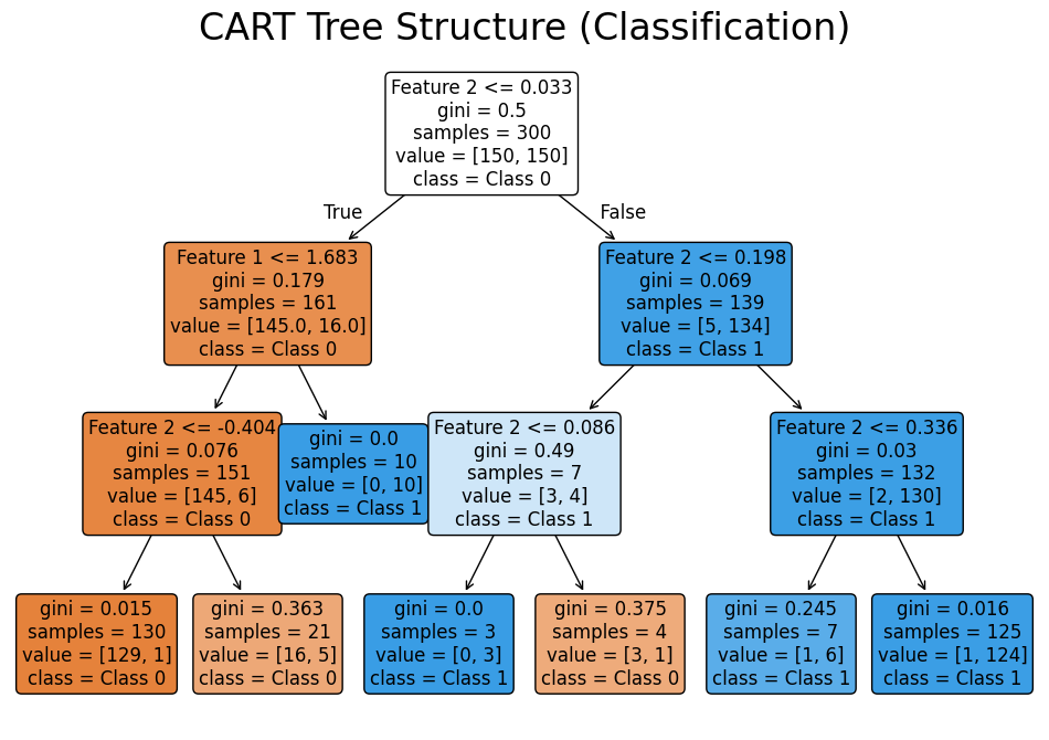
The tree visualization shows the hierarchical decision-making process, with each node displaying the splitting criterion and the resulting class distribution.
Example
Let's work through a concrete example to understand how CART builds a decision tree step by step. We'll use a simple classification problem with two features and three classes.
Dataset Setup
Consider the following training data:
| Sample | Feature 1 (X₁) | Feature 2 (X₂) | Class |
|---|---|---|---|
| 1 | 2.5 | 1.2 | A |
| 2 | 3.1 | 2.8 | B |
| 3 | 1.8 | 3.2 | A |
| 4 | 4.2 | 1.5 | C |
| 5 | 2.9 | 2.1 | B |
| 6 | 1.5 | 2.9 | A |
| 7 | 3.8 | 2.3 | C |
| 8 | 2.2 | 1.8 | A |
Step 1: Calculate Initial Gini Impurity
First, we calculate the Gini impurity for the root node (all samples):
- Class A: 4 samples (50%)
- Class B: 2 samples (25%)
- Class C: 2 samples (25%)
Step 2: Evaluate All Possible Splits
Split on X₁ ≤ 2.5:
Left child (X₁ ≤ 2.5): Samples 1, 3, 6, 8
- Class A: 4 samples (100%)
- Class B: 0 samples (0%)
- Class C: 0 samples (0%)
Right child (X₁ > 2.5): Samples 2, 4, 5, 7
- Class A: 0 samples (0%)
- Class B: 2 samples (50%)
- Class C: 2 samples (50%)
Weighted Gini impurity:
Information gain:
Split on X₂ ≤ 2.0:
Left child (X₂ ≤ 2.0): Samples 1, 4, 8
- Class A: 2 samples (66.7%)
- Class B: 0 samples (0%)
- Class C: 1 sample (33.3%)
Right child (X₂ > 2.0): Samples 2, 3, 5, 6, 7
- Class A: 2 samples (40%)
- Class B: 2 samples (40%)
- Class C: 1 sample (20%)
Weighted Gini impurity:
Information gain:
Step 3: Select Best Split
The split on X₁ ≤ 2.5 provides the highest information gain (0.375), so we choose this as our first split.
Step 4: Continue Building the Tree
We now have two child nodes. The left child (X₁ ≤ 2.5) is already pure (all samples are class A), so it becomes a leaf node. The right child (X₁ > 2.5) still has mixed classes and needs further splitting.
For the right child, we repeat the process:
- Current samples: 2, 4, 5, 7
- Classes: B, C, B, C
The best split would be on X₂ ≤ 2.1, which would separate the classes perfectly.
Final Tree Structure
Root: X₁ ≤ 2.5?
├── Yes → Class A (Leaf)
└── No → X₂ ≤ 2.1?
    ├── Yes → Class B (Leaf)
    └── No → Class C (Leaf)
This example demonstrates how CART greedily selects splits that maximize information gain at each step, ultimately creating a tree that perfectly classifies the training data.
Implementation in Scikit-learn
Scikit-learn provides a comprehensive implementation of CART through the DecisionTreeClassifier and DecisionTreeRegressor classes. Let's walk through how to build, train, and evaluate decision trees for both classification and regression tasks.
Data Preparation
We'll start by importing the necessary libraries and creating synthetic datasets for both classification and regression examples.
Classification Implementation
Now let's build a decision tree classifier. We'll configure several key parameters to control the tree's complexity and prevent overfitting.
Let's examine the classification performance:
The test accuracy shows how well the model performs on unseen data. The cross-validation scores provide a more robust estimate of model performance by averaging results across multiple train-test splits. The standard deviation indicates the stability of the model's performance—lower values suggest more consistent predictions across different data subsets.
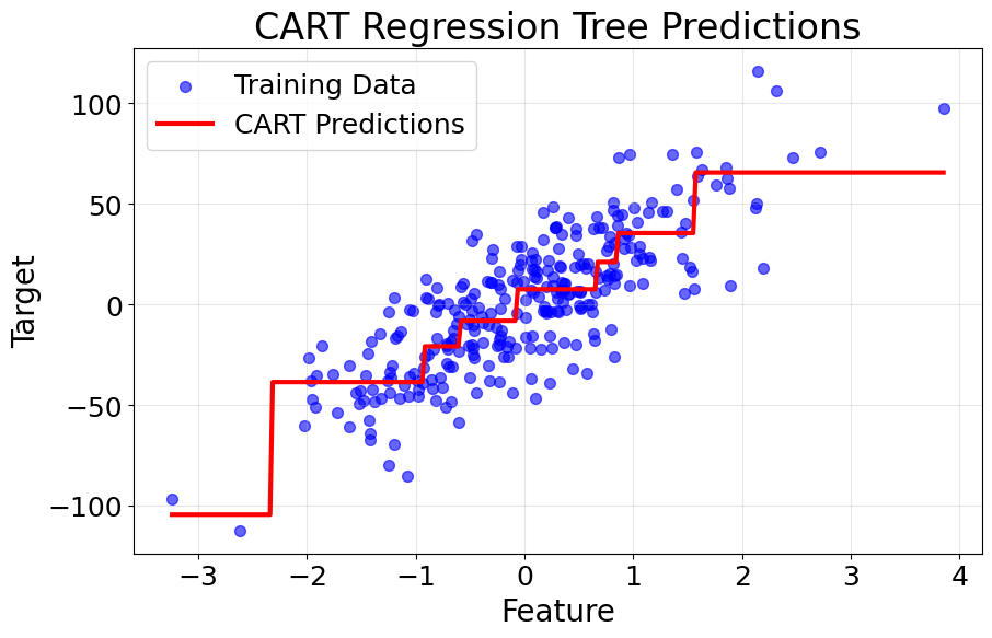
Regression Implementation
For regression tasks, we use DecisionTreeRegressor with similar parameters but adjusted for the continuous target variable.
Let's examine the regression performance:
The RMSE (Root Mean Squared Error) measures the average prediction error in the same units as the target variable. Lower RMSE values indicate better predictive accuracy. The cross-validation RMSE provides a more reliable estimate of how the model will perform on new data, with the standard deviation showing the consistency of predictions across different data splits.
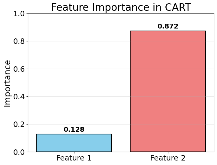
Feature Importance Analysis
Decision trees automatically calculate feature importance based on how much each feature reduces impurity across all splits.
These importance scores indicate which features contribute most to the model's predictions. Features with higher scores have a greater influence on the decision-making process. In this example, the scores show how the tree prioritizes different features when making splits.
Tree Visualization
Visualizing the tree structure helps understand the decision-making process:
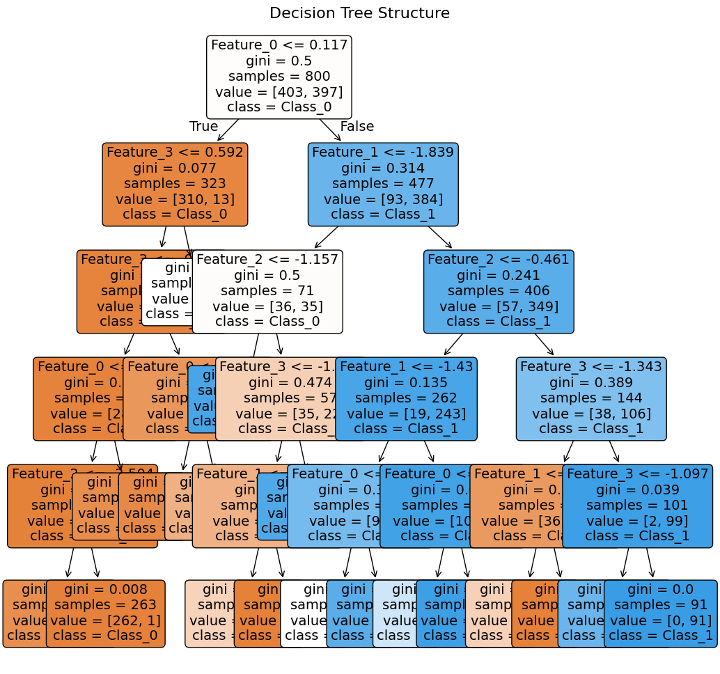
Note: This visualization is intended for illustrative purposes. It's normal if not all feature details are visible in the tree plot.
The tree visualization shows the complete decision-making hierarchy. Each node displays the splitting criterion (feature and threshold), the Gini impurity, the number of samples, and the class distribution. The color intensity indicates node purity—darker colors represent more homogeneous nodes. This visual representation makes it easy to trace any prediction back through the specific sequence of decisions that led to it.
Key Parameters
Below are the main parameters that control how CART decision trees work and perform.
-
max_depth: Maximum depth of the tree (default: None). Limiting depth prevents overfitting by restricting tree complexity. Start with values like 5-10 and adjust based on cross-validation performance. -
min_samples_split: Minimum samples required to split an internal node (default: 2). Higher values prevent the tree from creating splits on small subsets, reducing overfitting. Values of 10-20 work well for most datasets. -
min_samples_leaf: Minimum samples required in a leaf node (default: 1). This ensures leaves have sufficient data for reliable predictions. Values of 5-10 help prevent overfitting while maintaining predictive power. -
max_features: Number of features to consider for the best split (default: None for all features). Options include'sqrt'(square root of total features),'log2'(log base 2 of total features), or an integer. Using fewer features can reduce overfitting and speed up training. -
criterion: Function to measure split quality. For classification:'gini'(default) or'entropy'. For regression:'squared_error'(default) or'absolute_error'. Gini and squared_error are computationally faster and work well in most cases. -
random_state: Seed for reproducibility (default: None). Set to an integer to ensure consistent results across runs, especially important when usingmax_featureswith randomization. -
min_impurity_decrease: Minimum impurity decrease required for a split (default: 0.0). A node will split only if the decrease in impurity is greater than or equal to this value. Useful for pruning weak splits. -
ccp_alpha: Complexity parameter for minimal cost-complexity pruning (default: 0.0). Higher values result in more aggressive pruning, creating simpler trees. Use cross-validation to find the optimal value.
Key Methods
The following are the most commonly used methods for interacting with CART decision tree models.
-
fit(X, y): Trains the decision tree on the training data X and target values y. The tree is built by recursively finding the best splits according to the specified criterion. -
predict(X): Returns predicted class labels (classification) or values (regression) for input data X. For classification, returns the majority class in the leaf node. For regression, returns the mean value of samples in the leaf node. -
predict_proba(X): Returns probability estimates for each class (classification only). Probabilities are calculated as the fraction of training samples of each class in the leaf node. Useful for setting custom decision thresholds or understanding prediction confidence. -
score(X, y): Returns the mean accuracy (classification) or R² score (regression) on the given test data. Provides a quick way to evaluate model performance. -
get_depth(): Returns the depth of the decision tree. Useful for understanding tree complexity and diagnosing potential overfitting. -
get_n_leaves(): Returns the number of leaves in the decision tree. More leaves indicate a more complex model that may be overfitting. -
apply(X): Returns the index of the leaf that each sample ends up in. Useful for understanding which samples follow similar decision paths or for creating custom features based on tree structure.
Practical Applications
When to Use CART
CART models excel in scenarios where interpretability and transparency are paramount. In healthcare applications, decision trees help clinicians understand diagnostic reasoning, making it easier to validate recommendations and explain decisions to patients. The ability to translate tree structures into simple if-then rules makes CART valuable in regulatory environments where model decisions must be explainable to auditors and stakeholders. For example, a credit scoring model built with CART can clearly show why an application was rejected, which is often a legal requirement.
CART is particularly effective for exploratory data analysis and initial model development. The tree structure naturally reveals which features are most important for predictions and how they interact, providing insights that can guide feature engineering for more complex models. When working with small to medium-sized datasets (typically under 10,000 samples), CART can deliver competitive performance while maintaining complete transparency. The algorithm also handles mixed data types naturally, making it suitable for datasets containing both categorical and numerical features without extensive preprocessing.
However, CART is less appropriate when maximum predictive accuracy is the primary goal, as ensemble methods like Random Forest or Gradient Boosting typically outperform single trees. Avoid CART when you need to extrapolate beyond the training data range, since decision trees can only make predictions within the feature space they've observed. For problems with complex geometric patterns or diagonal decision boundaries, algorithms like Support Vector Machines or Neural Networks may be more effective due to CART's limitation to axis-parallel splits.
Best Practices
To achieve optimal results with CART, start by carefully tuning the tree depth using cross-validation. Begin with max_depth values between 3 and 10, as deeper trees tend to overfit while shallow trees may underfit. Set min_samples_split to values between 10 and 50 to prevent the tree from creating splits based on small subsets of data, which often capture noise rather than meaningful patterns. Similarly, configure min_samples_leaf to require at least 5-10 samples in each leaf node, ensuring that predictions are based on sufficient evidence.
Use cross-validation to evaluate model performance rather than relying solely on training accuracy. A tree that achieves very high training accuracy may be overfitting and will likely perform poorly on new data. Consider using cost-complexity pruning by setting the ccp_alpha parameter, which removes branches that provide minimal improvement in predictive power. Start with ccp_alpha=0.0 and gradually increase it while monitoring cross-validation scores to find the optimal balance between model complexity and generalization.
For classification tasks, the default Gini impurity criterion works well in most cases and is computationally faster than entropy. However, if you're specifically interested in maximizing information gain or working with highly imbalanced classes, entropy may provide better results. When dealing with categorical features that have many categories, consider grouping rare categories together or using target encoding to reduce cardinality, as high-cardinality features can dominate the splitting process and lead to overfitting.
Data Requirements and Preprocessing
CART handles various data types with minimal preprocessing requirements, but certain considerations can significantly improve performance. While the algorithm doesn't strictly require feature scaling due to its use of rank-based splits, standardization can be beneficial when features have vastly different ranges, particularly if you plan to compare feature importance values across features. For categorical features, CART naturally handles them through binary splits, but encoding strategies become important when categories number in the hundreds or thousands.
Missing values require careful attention, as scikit-learn's implementation doesn't natively support them. You'll need to either impute missing values or use surrogate splits (available in some implementations). For imputation, consider using median values for numerical features and mode for categorical features, or more sophisticated methods like iterative imputation if missingness patterns are informative. When dealing with outliers, CART is relatively robust compared to distance-based algorithms, as extreme values only affect the specific splits where they appear rather than the entire model.
The algorithm performs best when the target variable has sufficient representation across all classes (for classification) or a reasonable distribution (for regression). For highly imbalanced classification problems, consider using class weights or resampling techniques before training. For regression, if the target variable spans several orders of magnitude, log-transforming it may help the tree create more meaningful splits and improve prediction accuracy on the original scale.
Common Pitfalls
One frequent mistake is allowing trees to grow too deep without proper regularization, resulting in models that memorize training data rather than learning generalizable patterns. This manifests as very high training accuracy but poor test performance. To avoid this, set explicit constraints on tree depth and minimum samples per split, and validate performance using cross-validation rather than a single train-test split. Another common error is selecting hyperparameters based solely on training performance, which typically leads to overfitting.
Relying exclusively on a single decision tree for production applications can be problematic due to the algorithm's high variance. Small changes in training data can produce dramatically different tree structures, making predictions unstable over time. If you observe significant performance fluctuations when retraining on slightly different data, consider using ensemble methods or implementing model averaging strategies. Additionally, practitioners sometimes overlook the importance of feature engineering, assuming that CART will automatically discover all relevant patterns. While the algorithm does capture interactions, creating domain-specific features often substantially improves performance.
Ignoring the interpretability-complexity tradeoff is another pitfall. Some users add numerous regularization parameters and complex preprocessing pipelines that negate CART's primary advantage of interpretability. If your final model requires extensive documentation to explain, you may have lost the benefit of using a decision tree in the first place. Finally, failing to validate that the tree's learned rules align with domain knowledge can lead to models that are mathematically optimal but practically meaningless. Review the top splits and feature importance to ensure they make sense in the context of your problem.
Computational Considerations
CART's computational complexity for training is O(n × m × log n) where n is the number of samples and m is the number of features, making it efficient for small to medium datasets. For datasets under 10,000 samples, training typically completes in seconds on modern hardware. However, performance degrades for very large datasets (>100,000 samples) or high-dimensional feature spaces (>1,000 features), where the algorithm must evaluate many potential splits at each node. In such cases, consider using sampling strategies to train on representative subsets or limiting the number of features considered at each split using the max_features parameter.
Memory requirements are generally modest, as the tree structure itself is compact—each node only stores the split criterion, threshold, and pointers to child nodes. A typical tree with 100 leaf nodes requires only a few kilobytes of memory. However, the training process requires keeping the full dataset in memory, which can be limiting for very large datasets. For datasets that don't fit in memory, consider using out-of-core learning approaches or distributed computing frameworks, though this often negates the simplicity advantage of CART.
Prediction time scales linearly with tree depth, making CART suitable for real-time applications where low latency is critical. A typical tree with depth 10 requires only 10 comparisons to make a prediction, which completes in microseconds. This makes CART particularly attractive for embedded systems, mobile applications, or high-throughput prediction scenarios. However, be aware that extremely deep trees (depth >20) or very wide trees (many branches at each node) can slow predictions, especially when processing large batches of data.
Performance and Deployment Considerations
Evaluating CART performance requires using appropriate metrics for your task. For classification, examine not just accuracy but also precision, recall, and F1-scores for each class, particularly if classes are imbalanced. The confusion matrix reveals which classes the tree confuses, often highlighting areas where additional features or different split criteria might help. For regression, consider both RMSE (which penalizes large errors) and MAE (which treats all errors equally) to understand the error distribution. Always compare performance against a simple baseline, such as predicting the majority class or mean value, to ensure the tree is learning meaningful patterns.
When deploying CART models to production, monitor for data drift that could degrade performance over time. Since trees cannot adapt to new patterns without retraining, establish a schedule for model updates based on performance monitoring. Track key metrics like prediction accuracy, feature distributions, and the proportion of samples reaching each leaf node. Significant changes in these metrics indicate that retraining may be necessary. Consider implementing A/B testing when deploying new tree versions to validate that changes improve real-world performance.
The interpretability of CART makes it well-suited for applications requiring model explainability, but this requires proper documentation. Export the tree structure as a set of rules and validate that they align with domain expertise. In regulated industries, maintain audit trails showing how the tree was trained, which hyperparameters were selected, and how performance was validated. For critical applications, implement safeguards such as confidence thresholds—only making predictions when the leaf node contains sufficient samples or has high class purity. This conservative approach can prevent errors on edge cases where the tree's training data was sparse.
Summary
CART represents a fundamental approach to machine learning that prioritizes interpretability and simplicity. By recursively partitioning the feature space based on impurity measures, CART creates decision trees that can be easily understood and validated by domain experts. The algorithm's greedy nature, while sometimes leading to suboptimal solutions, makes it computationally efficient and transparent in its decision-making process.
The mathematical foundation of CART, based on Gini impurity for classification and variance reduction for regression, provides a principled approach to finding optimal splits. However, the algorithm's tendency toward overfitting and its sensitivity to small data changes require careful hyperparameter tuning and validation strategies. The built-in feature selection and natural handling of missing values make CART particularly suitable for exploratory data analysis and initial model development.
In practice, CART serves as an excellent starting point for many machine learning problems, especially when interpretability is crucial. While ensemble methods often provide superior predictive performance, CART's transparency and simplicity make it invaluable in domains where understanding the model's reasoning is as important as its accuracy. The algorithm's ability to handle mixed data types and create human-readable decision rules positions it as a versatile tool in the data scientist's toolkit, particularly valuable for stakeholder communication and regulatory compliance scenarios.
Quiz
Ready to test your understanding of CART? Take this quick quiz to reinforce what you've learned about classification and regression trees.

Comments