Numerical Methods in Finance: Algorithms for Pricing & Risk

Many problems in quantitative finance lack closed-form analytical solutions. When you need to find the yield-to-maturity of a bond, extract the implied volatility from an option price, or value a complex derivative, you often encounter equations that cannot be solved algebraically. Numerical methods provide systematic algorithms to approximate these solutions to arbitrary precision.

These techniques form the computational backbone of modern finance. Every trading platform that displays implied volatilities runs root-finding algorithms thousands of times per second. Every risk management system that constructs yield curves relies on interpolation methods. Every exotic derivative pricing engine uses numerical integration when analytical formulas are unavailable.

This chapter introduces three foundational categories of numerical methods: root-finding algorithms for solving equations, interpolation techniques for constructing continuous curves from discrete data, and numerical integration for computing definite integrals. You'll learn both the mathematical foundations and practical implementations, with applications to real financial problems including bond pricing, options valuation, and curve construction.

Root-finding algorithms solve equations of the form $f(x) = 0$, where you seek the value $x^*$ such that the function equals zero. In finance, these appear whenever you need to invert a pricing formula. Given an observed market price, what input parameter produces that price? This question is central to financial calculations, from basic bond analytics to derivatives pricing.

The challenge arises because financial pricing formulas typically express price as a function of some underlying parameter (yield, volatility, or credit spread), but markets quote prices directly. To convert between prices and rates or volatilities, you must solve the inverse problem: given the price, find the parameter. When the forward function is a complex nonlinear expression, its inverse rarely has a closed-form solution, and numerical methods become essential.

Consider the bond pricing equation:

where:

• $P$: observed market price of the bond
• $C$: periodic coupon payment
• $F$: face value (par value) of the bond
• $T$: total number of payment periods until maturity
• $y$: yield-to-maturity (the discount rate we seek)

The first term sums the present values of all coupon payments, while the second term adds the present value of the face value repaid at maturity. This formula embodies the fundamental principle of fixed-income valuation: a bond's fair price equals the present value of all its future cash flows, discounted at a rate that reflects the required return. Finding $y$ analytically is impossible because the equation is a polynomial of degree $T$. You know $P$ from the market, but solving for $y$ analytically is impossible for most bonds. For a 10-year bond with semi-annual payments, you face a polynomial equation of degree 20, beyond the reach of algebraic techniques. You must use numerical methods.

Similarly, the Black-Scholes formula gives option price as a function of volatility $\sigma$:

where:

• $C$: call option price
• $S_0$: current stock price
• $K$: strike price
• $T$: time to expiration
• $r$: risk-free interest rate
• $N(\cdot)$: cumulative standard normal distribution function
• $d_1, d_2$: parameters depending on volatility $\sigma$ (defined later)

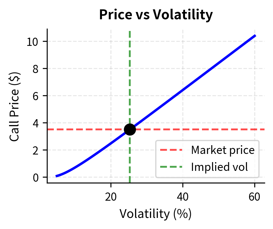
Given an observed option price $C_{market}$, finding the implied volatility $\sigma_{imp}$ requires solving $C(\sigma) - C_{market} = 0$. The Black-Scholes formula involves the standard normal cumulative distribution function, which itself has no closed-form inverse. Combined with the complex dependence of $d_1$ and $d_2$ on $\sigma$, the resulting equation demands numerical solution. This problem of finding the volatility implied by a market price is solved billions of times daily across global options markets.

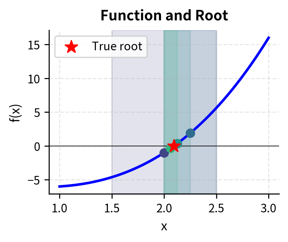
The bisection method is the simplest and most robust root-finding algorithm. It exploits the intermediate value theorem: if a continuous function $f$ has opposite signs at two points $a$ and $b$, then it must cross zero somewhere between them. This elegant mathematical principle guarantees that a root exists within the interval, providing the foundation for a systematic search strategy.

The intuition behind bisection is straightforward. If you know the root lies somewhere in an interval, the best way to narrow down its location is to check the midpoint. Depending on which half contains the root, you discard the other half and repeat. Each iteration cuts the uncertainty in half, inexorably converging toward the answer. This divide-and-conquer approach trades speed for certainty. Bisection may be slow, but it never fails when properly initialized.

The algorithm proceeds by repeatedly halving the interval:

1. Start with an interval $[a, b]$ where $f(a)$ and $f(b)$ have opposite signs
2. Compute the midpoint $c = \frac{a + b}{2}$
3. Evaluate $f(c)$
4. If $f(c)$ has the same sign as $f(a)$, replace $a$ with $c$; otherwise replace $b$ with $c$
5. Repeat until the interval is sufficiently small

Step 4 requires careful attention. Since $f(a)$ and $f(b)$ have opposite signs and the function is continuous, the root must lie between them. After computing $f(c)$, we ask: which half-interval still brackets the root? If $f(c)$ shares the same sign as $f(a)$, then the root lies between $c$ and $b$ (where signs still differ). Conversely, if $f(c)$ shares the same sign as $f(b)$, the root lies between $a$ and $c$. Either way, we've reduced the search interval by exactly half while maintaining the crucial sign-change property.

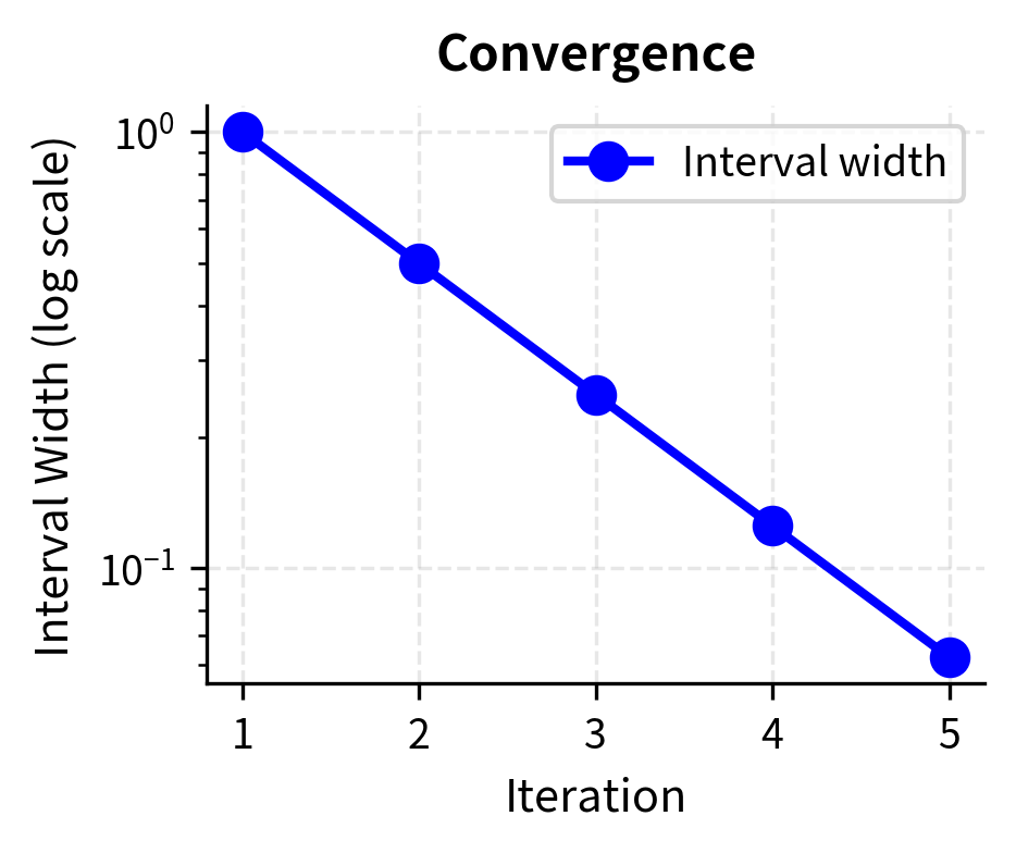
Each iteration halves the interval width, so after $n$ iterations, the error is at most:

where:

• $b-a$: initial interval width
• $n$: number of iterations performed
• $2^n$: factor by which the interval shrinks after $n$ halvings To achieve precision $\epsilon$, you need approximately $\log_2\left(\frac{b-a}{\epsilon}\right)$ iterations.

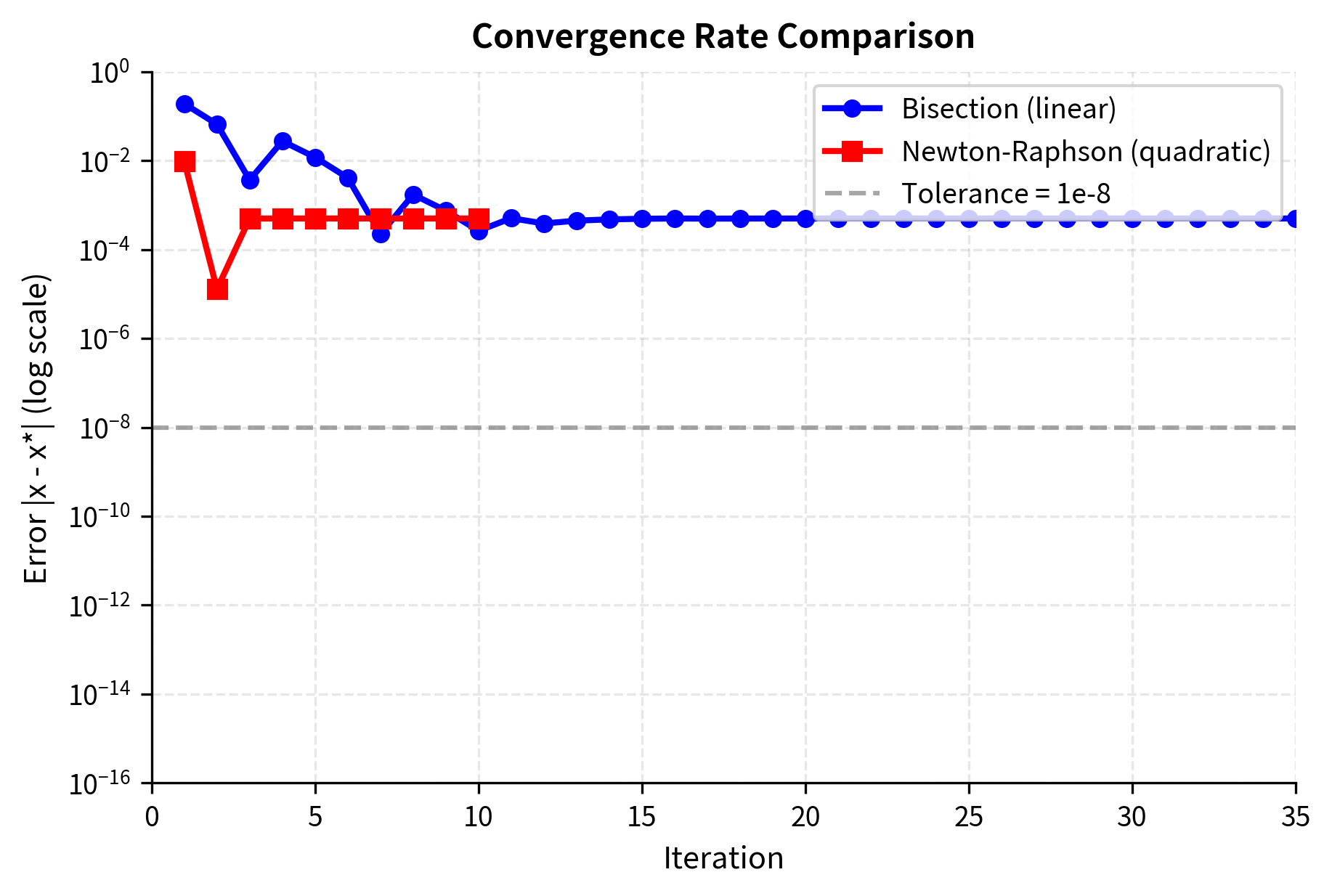
This logarithmic relationship means bisection is reliable but slow: achieving 10 decimal places of accuracy requires about 33 iterations regardless of the function. The method treats every function identically: it does not exploit any special structure like smoothness or convexity. A rapidly varying function and a nearly constant one require the same number of iterations for a given precision. This indifference to the function's character is both a strength (universal applicability) and a weakness (missed opportunities for acceleration).

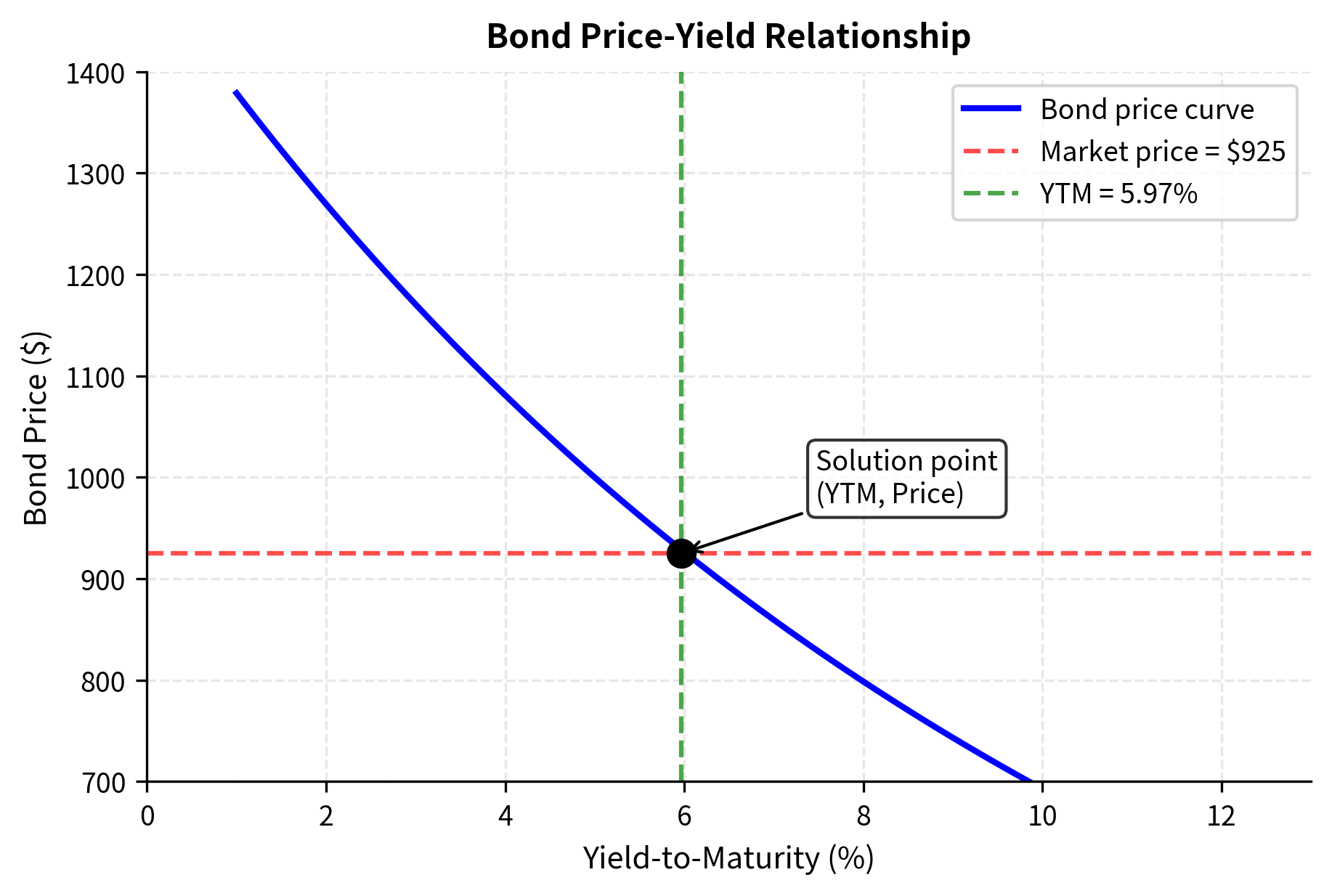
Let's implement bisection to find the yield-to-maturity of a bond:

Now let's apply this to a concrete example. Consider a 10-year bond with a 5% annual coupon, $1,000 face value, trading at$925:

The bond trades below par (at a discount), so the yield exceeds the coupon rate. The bisection method converged in about 30 iterations to find a YTM of approximately 5.97%. This result makes economic sense: investors demand a higher effective return than the stated coupon rate to compensate for the discount purchase price. Over the bond's life, they receive not only the coupon payments but also the capital gain from the price rising toward par at maturity.

While bisection is reliable, it converges slowly. The Newton-Raphson method achieves much faster convergence by using derivative information. The key insight is that the derivative tells us not just where the function is, but where it's going. By using this directional information, we can take informed steps toward the root rather than blindly halving intervals.

The geometric intuition is illuminating. At any point $x_n$, we can approximate the function by its tangent line, a linear approximation that matches both the function's value and its slope at that point. Where does this tangent line cross zero? That crossing point becomes our next estimate $x_{n+1}$. If the function is reasonably well-behaved near the root, the tangent line provides an excellent local approximation, and following it leads us closer to the root.

Starting from an initial guess $x_0$, each iteration updates:

where:

• $x_n$: current estimate of the root
• $f(x_n)$: function value at current estimate
• $f'(x_n)$: derivative of function at current estimate
• $x_{n+1}$: improved estimate after one iteration

Geometrically, this finds where the tangent line to $f$ at $x_n$ crosses the x-axis. The ratio $f(x_n)/f'(x_n)$ represents how far to step: a large function value requires a larger step, and a steep slope (large derivative) means we are close and need only a small step. To understand why, consider that the tangent line equation is $y = f(x_n) + f'(x_n)(x - x_n)$. Setting $y = 0$ and solving for $x$ yields exactly the Newton-Raphson update formula. The method thus asks: if the function behaved exactly like its tangent line, where would the root be?

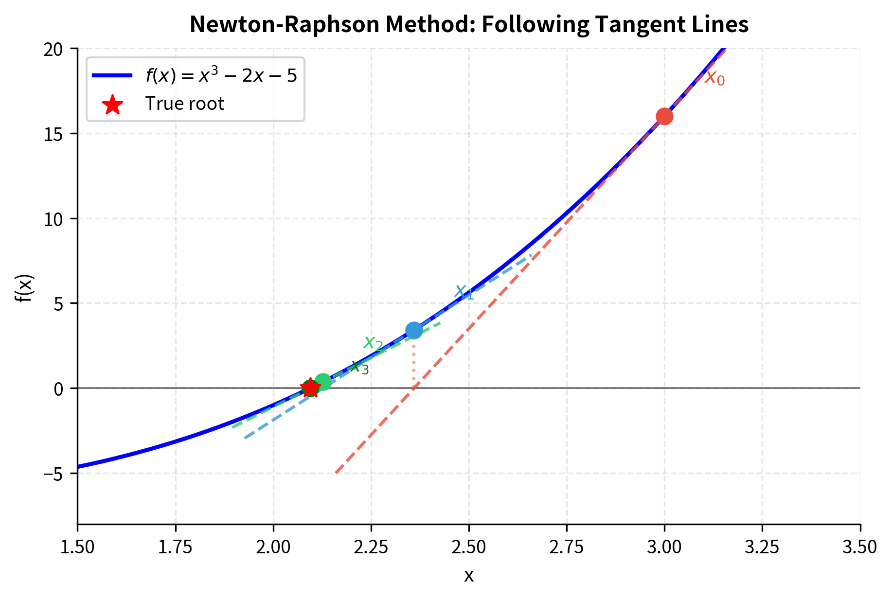
Near a simple root, Newton-Raphson exhibits quadratic convergence: the number of correct digits roughly doubles with each iteration.

This property explains why Newton-Raphson is faster than bisection. Bisection adds roughly one bit of precision per iteration (linear convergence), while Newton-Raphson adds roughly as many new bits as it already has (quadratic convergence). Once you're close to the root, convergence becomes explosive.

The main requirement is computing the derivative $f'(x)$. For bond pricing, the derivative of price with respect to yield is:

where:

• $\frac{dP}{dy}$: rate of change of bond price with respect to yield (negative of dollar duration)
• $t$: time period index
• $C$: periodic coupon payment
• $T$: total number of periods
• $F$: face value
• $(1+y)^{t+1}$: discount factor raised to power $t+1$ (one more than in the price formula due to differentiation)

This derivative, known as the bond's dollar duration (up to a sign), measures price sensitivity to yield changes. The negative sign indicates that prices fall when yields rise, a fundamental inverse relationship in fixed income. Each term is weighted by its time to payment $t$, reflecting that longer-dated cash flows are more sensitive to yield changes. This makes intuitive sense: a payment far in the future is discounted many times, so any change in the discount rate compounds over more periods.

The derivative formula emerges directly from applying the power rule to each term in the bond pricing equation. For a single cash flow $CF$ at time $t$, we have $\frac{d}{dy}[CF \cdot (1+y)^{-t}] = -t \cdot CF \cdot (1+y)^{-(t+1)}$. Summing over all cash flows gives the complete expression.

Newton-Raphson typically converges in 4-6 iterations compared to 25-30 for bisection. This efficiency matters when you are computing implied volatilities for thousands of options in real-time. The computational savings compound dramatically across an entire options chain, where a trading desk might need fresh implied volatilities for hundreds of strikes across multiple expirations, updated continuously throughout the trading day.

Implied volatility calculation is the canonical application of root-finding in options trading. Every options desk needs to convert between prices and volatilities rapidly. Traders think in terms of volatility, the natural unit for comparing options across different strikes, expirations, and underlying assets. But markets quote prices. The translation between these two representations happens through implied volatility calculation, making root-finding algorithms a critical piece of trading infrastructure.

The Black-Scholes formula for a European call option is:

where:

• $C$: call option price
• $S_0$: current stock price
• $K$: strike price of the option
• $T$: time to expiration in years
• $r$: risk-free interest rate (continuously compounded)
• $\sigma$: volatility of the underlying asset (the parameter we seek)
• $d_1 = \frac{\ln(S_0/K) + (r + \sigma^2/2)T}{\sigma\sqrt{T}}$: measures how far in-the-money the option is, adjusted for drift and volatility
• $d_2 = d_1 - \sigma\sqrt{T}$: adjusts $d_1$ for the volatility effect over the option's lifetime
• $N(\cdot)$: cumulative standard normal distribution function

The first term $S_0 N(d_1)$ represents the expected stock value at expiration (conditional on exercise), while $Ke^{-rT}N(d_2)$ is the present value of the strike payment weighted by the probability of exercise. The parameters $d_1$ and $d_2$ encode how likely the option is to finish in the money, measured in standard deviations of the log-price distribution. Notice that both depend on volatility in complex ways. The parameter $\sigma$ appears in the numerator, the denominator, and implicitly through the $N(\cdot)$ function. This tangled dependence makes analytical inversion impossible.

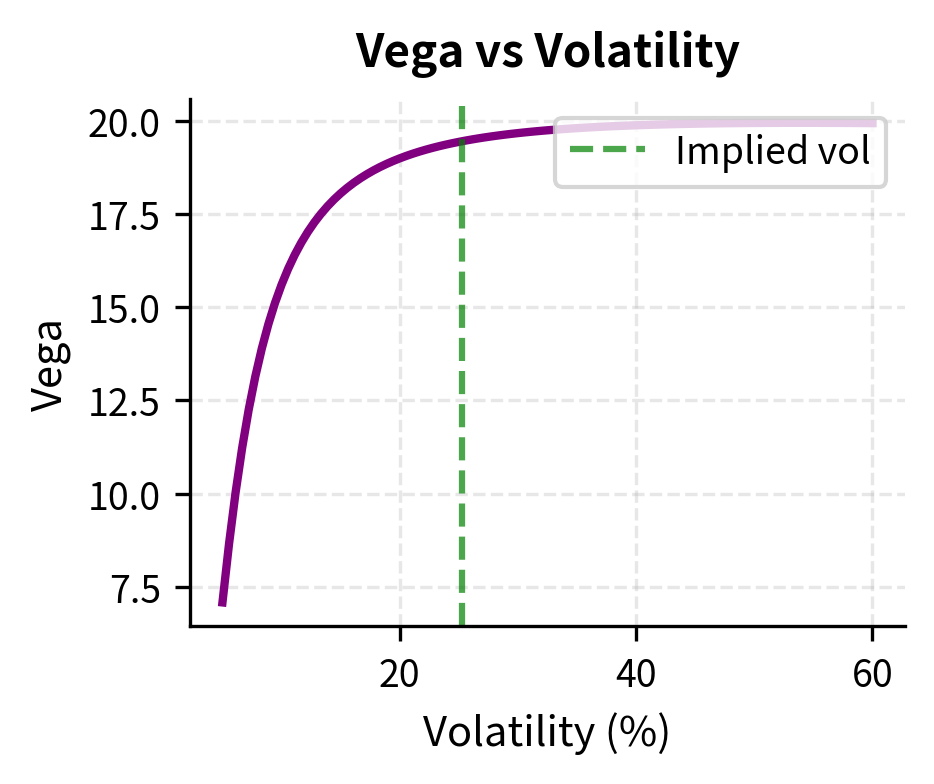
To use Newton-Raphson, we need the derivative of the option price with respect to volatility, known as vega:

where:

• $n(\cdot)$: standard normal probability density function $n(x) = \frac{1}{\sqrt{2\pi}}e^{-x^2/2}$
• $S_0 \sqrt{T}$: scales the sensitivity by stock price and time horizon
• $n(d_1)$: peaks when the option is at-the-money and decays for deep in/out-of-the-money options

Vega is always positive because higher volatility increases option value. This makes economic sense: options are bets on movement, and more volatility means more potential movement in either direction. Since the option holder benefits from favorable moves but has limited downside (the premium paid), increased uncertainty is valuable. Vega peaks for at-the-money options near expiration, which explains why Newton-Raphson struggles for deep out-of-the-money options where vega approaches zero. When the derivative is tiny, the Newton-Raphson step becomes enormous, potentially overshooting the valid range of volatilities entirely.

The simplicity of the vega formula, despite the complexity of the Black-Scholes price itself, reflects a deep result in stochastic calculus related to the Girsanov theorem. This has practical consequences: computing the exact derivative costs almost nothing beyond computing the price, making Newton-Raphson highly efficient for this problem.

Let's calculate implied volatility for a sample option:

The algorithm converged in just a few iterations. This efficiency is crucial because trading systems may need to compute implied volatilities for entire option chains, potentially thousands of contracts, multiple times per second. Each time a quote updates anywhere in the chain, the entire volatility surface needs refreshing to maintain a consistent view of market expectations.

When implementing root-finding in production systems, several considerations arise.

Initial guess selection significantly affects Newton-Raphson convergence. For implied volatility, a reasonable starting point is 20-30% for equity options, adjusted based on the option's moneyness. Poor initial guesses can lead to divergence or convergence to invalid solutions (like negative volatility).

Hybrid methods combine the robustness of bisection with the speed of Newton-Raphson. Start with Newton-Raphson, and if the iterate leaves a reasonable range or the step is too large, fall back to bisection for a few iterations to stabilize.

Brent's method is a sophisticated hybrid that combines bisection, secant, and inverse quadratic interpolation. It guarantees convergence like bisection while typically achieving superlinear convergence. Most production systems use Brent's method or similar hybrids.

Interpolation constructs continuous functions from discrete data points. In finance, you observe prices or rates at specific points, but need values at other locations. A yield curve might have observed rates at 3-month, 6-month, 1-year, 2-year, 5-year, and 10-year maturities, but you need to price a bond maturing in 3.5 years. The market provides data at certain locations, and interpolation fills in the values between them.

The challenge goes beyond convenience. Financial instruments exist at arbitrary maturities and strikes, not just at the discrete points where we have direct market observations. A corporate treasurer hedging a loan with a specific maturity, a portfolio manager pricing an off-the-run bond, or a derivatives trader valuing an exotic option at an unusual strike: all require rates or volatilities at points not directly quoted. Interpolation bridges this gap, but the choice of interpolation method affects pricing, hedging, and risk management in subtle but important ways.

Linear interpolation connects adjacent data points with straight lines. Given points $(x_0, y_0)$ and $(x_1, y_1)$, the interpolated value at $x$ is:

where:

• $(x_0, y_0)$ and $(x_1, y_1)$: the two known data points bracketing $x$
• $x$: the point at which we want to interpolate
• $\frac{y_1 - y_0}{x_1 - x_0}$: the slope of the line connecting the two points
• $(x - x_0)$: horizontal distance from the left point

The formula starts at $y_0$ and adds the slope times the horizontal distance traveled. This geometric interpretation makes linear interpolation intuitive: we're simply walking along the straight line connecting two known points. The rate of change (slope) is constant within each segment, jumping discontinuously as we cross from one segment to the next.

This can be written as a weighted average:

where:

• $t = \frac{x - x_0}{x_1 - x_0}$: interpolation parameter ranging from 0 to 1
• When $t = 0$: $x = x_0$ and $y = y_0$ (at the left endpoint)
• When $t = 1$: $x = x_1$ and $y = y_1$ (at the right endpoint)
• When $t = 0.5$: $x$ is the midpoint and $y$ is the average of $y_0$ and $y_1$

This weighted average form shows how linear interpolation works. The result is a convex combination of the two endpoint values, with weights determined by relative position. The parameter $t$ measures progress from the left point to the right point, normalized to the unit interval. This formulation generalizes naturally to higher dimensions and forms the basis for barycentric coordinates in computer graphics.

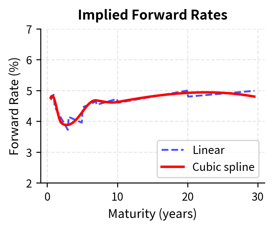
Linear interpolation is simple and computationally efficient, but it has a significant drawback. The interpolated curve has discontinuous first derivatives at the data points, creating "kinks." For many financial applications, this lack of smoothness is problematic. Consider computing the forward rate from a yield curve. The forward rate involves derivatives of the discount function, and kinks in the yield curve translate to jumps in forward rates. These artificial jumps have no economic meaning. They are purely artifacts of the interpolation method.

Cubic spline interpolation addresses the smoothness problem by fitting piecewise cubic polynomials that are continuous in both first and second derivatives. The name comes from a physical analogy: imagine bending a thin, flexible strip of material (a "spline") so that it passes through a set of fixed points. The strip naturally assumes a shape that minimizes bending energy, which turns out to be mathematically equivalent to the cubic spline solution.

Given $n$ data points, cubic splines fit $n-1$ cubic polynomials, each of the form:

where:

• $S_i(x)$: cubic polynomial on the interval $[x_i, x_{i+1}]$
• $a_i$: constant term, equals $y_i$ (the data value at $x_i$)
• $b_i$: linear coefficient, controls the slope at $x_i$
• $c_i$: quadratic coefficient, related to curvature
• $d_i$: cubic coefficient, allows the curvature to vary across the interval

A cubic polynomial has four coefficients, and we have $n-1$ such polynomials, giving $4(n-1)$ unknowns in total. To determine all these coefficients uniquely, we need $4(n-1)$ equations. These come from the interpolation and smoothness requirements that make splines so useful.

The coefficients are determined by requiring:

• Interpolation: each polynomial passes through its endpoint data
• Continuity: adjacent polynomials match at data points
• Smoothness: first and second derivatives match at interior data points
• Boundary conditions: typically "natural" splines with zero second derivatives at endpoints, or "clamped" splines with specified first derivatives

The interpolation conditions provide $2(n-1)$ equations (each polynomial must match the data at both its left and right endpoints). Derivative matching at the $n-2$ interior points adds $2(n-2)$ more equations (one each for first and second derivatives). This gives $2(n-1) + 2(n-2) = 4n - 6$ equations. The two boundary conditions supply the remaining two equations needed to determine all coefficients uniquely.

This creates a smooth curve that passes exactly through all data points, with no discontinuities in slope or curvature. The smoothness properties make cubic splines particularly valuable for computing Greeks and other derivatives-based quantities. Where linear interpolation would produce artificial jumps in forward rates, cubic splines yield smooth forward curves that behave more like actual market rates.

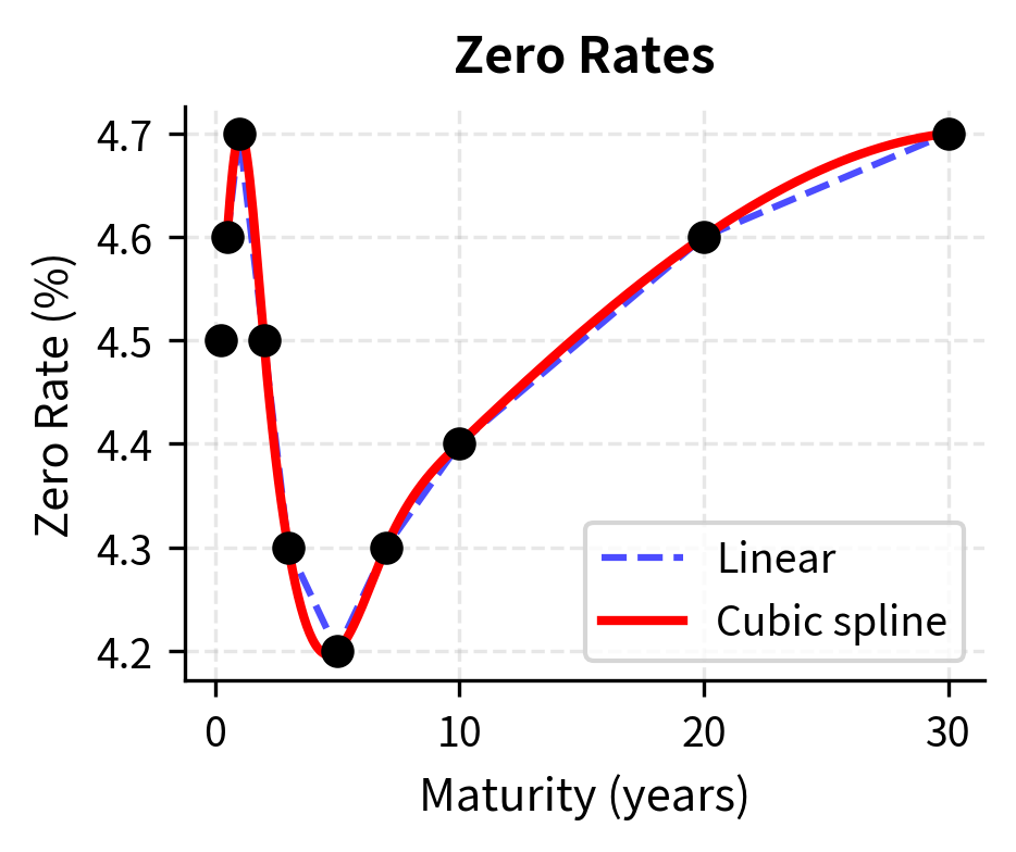
Let's visualize the difference between linear and cubic spline interpolation:

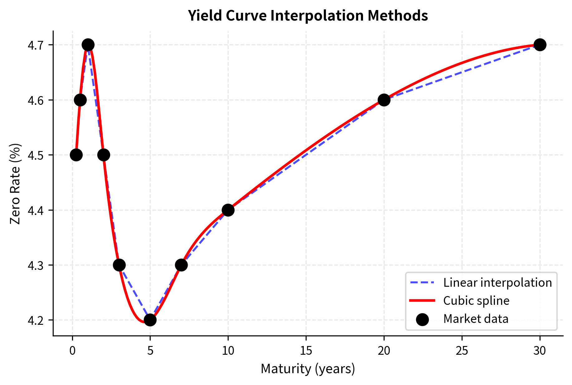
The cubic spline creates a smooth curve that follows the general shape of the data without the angular appearance of linear interpolation. Notice how the spline captures the inverted portion of the curve (rates dipping between 2-7 years) more naturally. The transition through the minimum is gradual, without the artificial corners that linear interpolation would produce at the 3-year and 5-year data points.

Volatility surfaces present a harder interpolation problem because they are two-dimensional: volatility depends on both strike price and time to expiration. Options traders need to interpolate these surfaces to price options at strikes and expirations not directly quoted in the market. A yield curve requires fitting a function of maturity alone, but a volatility surface requires fitting a function of two variables simultaneously.

The two-dimensional nature adds complexity. Not only must the surface pass through observed data points, but it should also exhibit sensible behavior between them: smoothness in both directions, no artificial valleys or peaks, and consistency with arbitrage constraints. The surface must make economic sense: volatility should not be negative, should not oscillate wildly between quoted points, and should follow the patterns (smiles, skews, term structure) that characterize real options markets.

The interpolated volatility of approximately 21% for this 9-month, slightly out-of-the-money option falls between the observed 6-month and 1-year values, as expected. The bivariate spline smoothly interpolates both the strike and expiration dimensions simultaneously, producing a value consistent with the surrounding observations in the volatility surface.

Let's visualize the full interpolated surface:

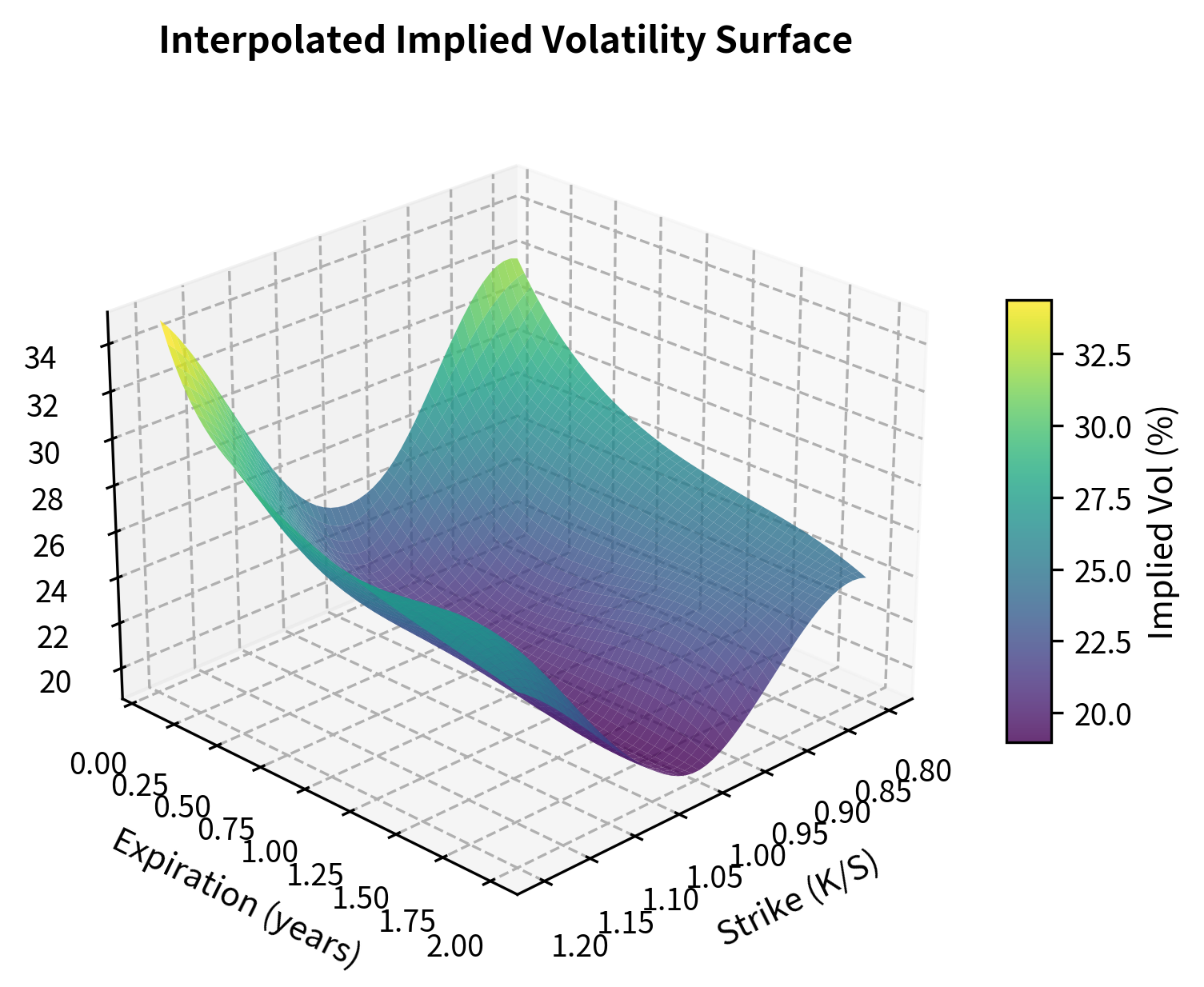
The surface displays the classic "volatility smile" pattern where out-of-the-money options (both puts with low K/S and calls with high K/S) have higher implied volatilities than at-the-money options. The smile flattens as expiration increases, a phenomenon known as the term structure of volatility. This flattening reflects the market's belief that while extreme moves are relatively more likely in the short term (perhaps due to jump risk or liquidity effects), over longer horizons the distribution looks more Gaussian and volatility becomes more uniform across strikes.

The choice of interpolation method depends on the application.

Linear interpolation is appropriate when:

• Speed is critical and you are doing millions of lookups
• The data is already dense enough that smoothness does not matter much
• You want to avoid oscillation artifacts that can occur with higher-order methods

Cubic splines are preferred when:

• Smoothness is important for risk calculations (Greeks require derivatives)
• You're constructing curves for pricing that will be used across many instruments
• Visual quality matters for reporting

Specialized financial interpolation methods exist for specific applications. For yield curves, monotone-preserving splines prevent spurious oscillations. For volatility surfaces, stochastic volatility models or SABR parameterization may be more appropriate than generic interpolation.

Numerical integration approximates definite integrals when analytical solutions are unavailable. In finance, this arises when computing expected values, pricing path-dependent options, or evaluating probability distributions. Integration is the continuous analog of summation. Many financial quantities are expressed as continuous sums over possible outcomes, weighted by their probabilities.

The connection between integration and expected values makes numerical integration central to derivatives pricing. Under risk-neutral valuation, the price of any derivative equals the discounted expected value of its payoff. When the expectation can be written as an integral, numerical integration provides a direct path to the price. Even when Monte Carlo simulation is the primary tool, numerical integration often handles sub-problems more efficiently.

Consider the expected payoff of an option under a probability distribution $p(S_T)$:

where:

• $\mathbb{E}[\text{Payoff}]$: expected value of the option payoff
• $S_T$: stock price at expiration time $T$
• $\text{Payoff}(S_T)$: option payoff as a function of terminal stock price
• $p(S_T)$: probability density function of the stock price at expiration

This integral accumulates the payoff at each possible terminal price, weighted by the probability of that price occurring. The integral runs from zero to infinity because stock prices are non-negative but have no upper bound. For simple European options under Black-Scholes, this integral has a closed form. But for more complex payoffs or distributions, numerical integration is necessary.

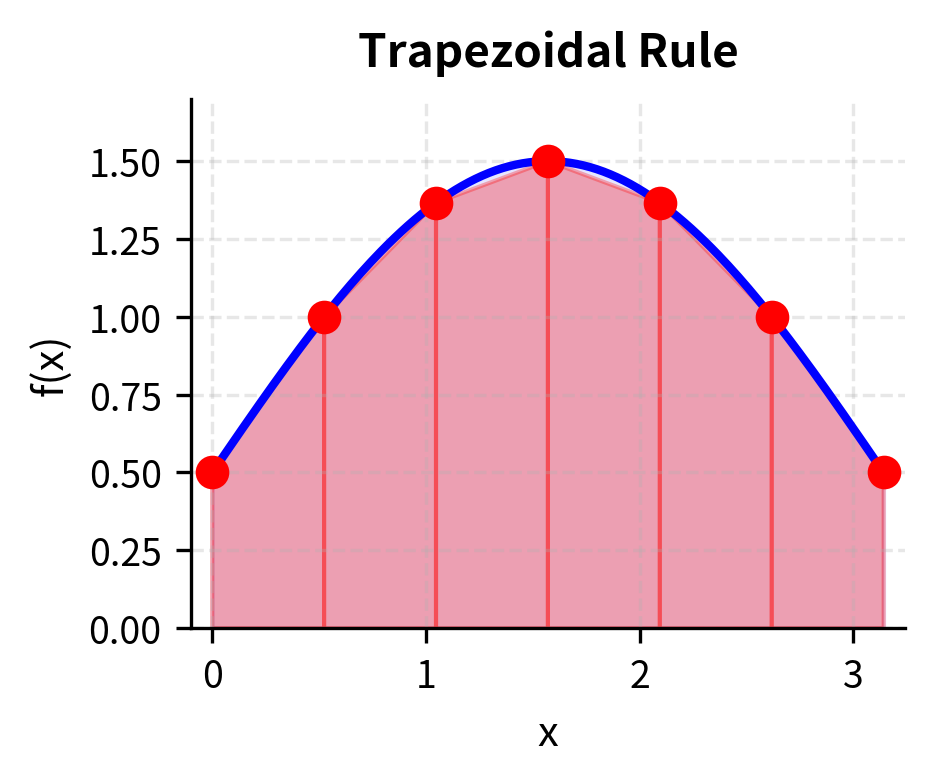
The trapezoidal rule approximates the area under a curve by dividing it into trapezoids. The key insight is that trapezoids—quadrilaterals with two parallel sides—provide a better approximation to curved regions than rectangles. Where a rectangle overestimates or underestimates the area depending on which corner matches the curve, a trapezoid averages between the two endpoints, typically achieving a more balanced approximation.

For an integral $\int_a^b f(x) \, dx$ with $n$ equally-spaced points $x_0 = a, x_1, ..., x_n = b$:

where:

• $h = \frac{b-a}{n}$: step size (width of each trapezoid)
• $f(x_0)$ and $f(x_n)$: function values at endpoints (each effectively weighted by $\frac{1}{2}$)
• $f(x_i)$ for $i = 1, \ldots, n-1$: function values at interior points (coefficient 2 appears because each interior point is shared by two adjacent trapezoids)

The factor of 2 for interior points arises because each interior point is shared by two adjacent trapezoids. The area of a single trapezoid with parallel sides $f(x_i)$ and $f(x_{i+1})$ is $\frac{h}{2}(f(x_i) + f(x_{i+1}))$; summing all trapezoids and collecting terms yields the formula above. The endpoints appear only once (each is the edge of only one trapezoid), while interior points appear twice (as the right edge of one trapezoid and the left edge of the next).

The trapezoidal rule has error $O(h^2)$. Doubling the number of points reduces the error by a factor of four. This relationship emerges from Taylor series analysis: the trapezoidal rule is exact for linear functions and makes errors proportional to the second derivative of the function, which determines how much the curve deviates from linearity.

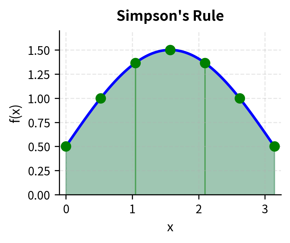
Simpson's rule achieves higher accuracy by fitting parabolas through groups of three points. Rather than approximating the curve with straight line segments, Simpson's rule uses quadratic polynomials that can capture curvature. Since any three points uniquely determine a parabola, we divide the interval into pairs of subintervals and fit a parabola to each trio of consecutive points.

For $n$ intervals (where $n$ must be even):

where:

• Odd-indexed points ($i = 1, 3, 5, ...$): weighted by 4 (midpoints of parabolic segments)
• Even-indexed points ($i = 2, 4, 6, ...$): weighted by 2 (shared endpoints between segments)
• Endpoints $f(x_0)$ and $f(x_n)$: weighted by 1

The 1-4-2-4-2-...-4-1 weighting pattern comes from integrating quadratic polynomials exactly. The coefficient 4 for odd-indexed points arises because these are the midpoints of each parabolic segment where the parabola contributes most. The coefficient 2 for even-indexed interior points reflects that these endpoints are shared by adjacent parabolic segments.

To understand why Simpson's rule uses these specific weights, consider integrating a parabola $p(x) = ax^2 + bx + c$ over an interval $[-h, h]$ centered at the origin. The exact integral equals $\frac{h}{3}[p(-h) + 4p(0) + p(h)]$, which is precisely the Simpson's rule formula applied to three points. By choosing weights that make the formula exact for parabolas, we ensure high accuracy for any function that is approximately quadratic over each pair of sub-intervals.

Simpson's rule has error $O(h^4)$. This makes it much more accurate than the trapezoidal rule for smooth functions. The fourth-order convergence means that halving the step size reduces the error by a factor of 16, an improvement over the factor of 4 achieved by the trapezoidal rule. This increased accuracy comes at at no extra cost: Simpson's rule requires the same function evaluations as the trapezoidal rule, just combined with different weights.

Gaussian quadrature achieves remarkable accuracy by choosing both the evaluation points and weights optimally. Rather than using equally-spaced points, it selects points (called nodes or abscissas) that maximize accuracy for polynomial functions. The key insight is that if you're free to choose where to evaluate the function, some choices are much better than others.

Consider the constraints. With $n$ function evaluations, we have $2n$ degrees of freedom to optimize (n node positions and n weights). If we want the formula to be exact for polynomials, we should use these degrees of freedom to handle the highest-degree polynomials possible. For equally-spaced points (where positions are fixed), we can only optimize the $n$ weights, achieving exactness for polynomials up to degree $n-1$. But by optimizing both positions and weights, Gaussian quadrature achieves exactness for polynomials up to degree $2n-1$—nearly twice as good.

For Gauss-Legendre quadrature on $[-1, 1]$:

where:

• $n$: number of quadrature points
• $x_i$: nodes (abscissas), roots of the $n$-th degree Legendre polynomial $P_n(x)$
• $w_i$: weights, computed to make the formula exact for polynomials up to degree $2n-1$

Example values:

• For $n = 2$: nodes at $x = \pm 1/\sqrt{3} \approx \pm 0.577$, weights $w = 1$
• For $n = 3$: nodes at $x = 0, \pm\sqrt{3/5} \approx \pm 0.775$, weights $w = 8/9, 5/9, 5/9$

The nodes are not equally spaced. They cluster toward the interval endpoints to control error near the boundaries where polynomial interpolation typically has the largest errors. This clustering is not arbitrary; it emerges from the mathematical requirement of exactness for high-degree polynomials, which forces the nodes to be roots of orthogonal polynomials (Legendre polynomials for the interval $[-1,1]$). The mathematics underlying Gaussian quadrature connects to the theory of orthogonal polynomials and approximation theory.

This formula is exact for polynomials of degree up to $2n-1$, which is highly efficient. With just $n$ function evaluations, we achieve the same accuracy as a $(2n-1)$-degree polynomial approximation. For smooth functions that are well-approximated by polynomials, this translates to high accuracy with very few evaluations.

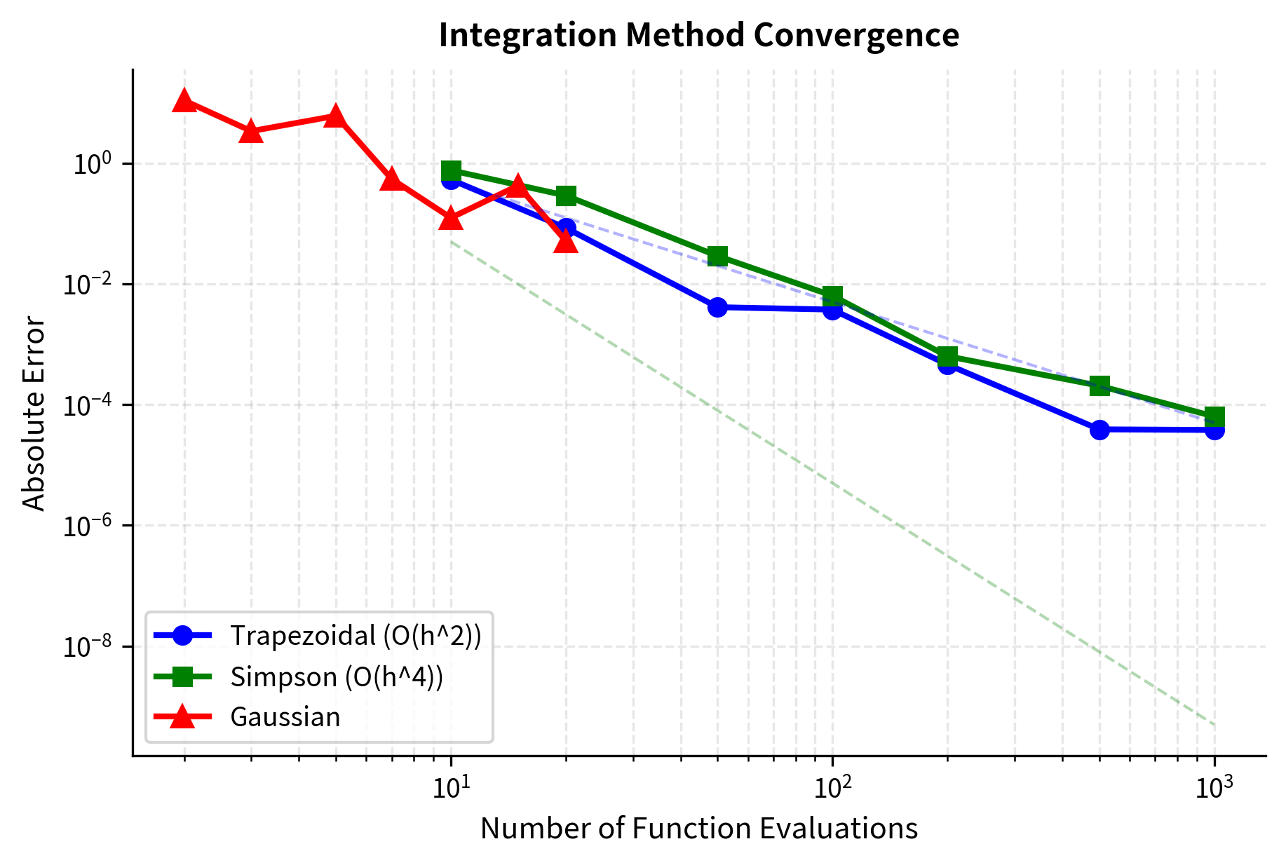
Let's compare these methods on a financial example: computing the expected payoff of a call option under a normal distribution of returns.

The results reveal the efficiency differences between methods. The trapezoidal rule requires 1000 points to achieve reasonable accuracy, while Simpson's rule reaches similar precision with just 100 points due to its O(h⁴) error convergence. Gaussian quadrature with just 20 points achieves accuracy comparable to Simpson's rule with 1000 points. This efficiency makes Gaussian quadrature the method of choice when function evaluations are expensive.

Integration arises throughout quantitative finance in several key areas:

Risk-neutral pricing expresses derivatives prices as discounted expected payoffs:

where:

• $V_0$: current value of the derivative
• $e^{-rT}$: discount factor from expiration to today
• $\mathbb{E}^{\mathbb{Q}}$: expectation under the risk-neutral probability measure
• $\text{Payoff}$: derivative's payoff at expiration, typically a function of the underlying asset price $S_T$

When payoffs are complex or the risk-neutral distribution doesn't yield closed forms, numerical integration computes these expectations.

Value at Risk (VaR) requires integrating the tail of a loss distribution:

where:

• $\text{VaR}_\alpha$: Value at Risk at confidence level $\alpha$
• $L$: portfolio loss (positive values = losses)
• $\alpha$: confidence level (typically 95% or 99%)
• $\inf$: infimum (smallest value satisfying the condition)

This definition says VaR is the smallest loss threshold such that the probability of exceeding it is at most $1-\alpha$.

While often computed via simulation, analytical approaches use numerical integration to evaluate the cumulative distribution function.

Probability transforms in copula models and risk aggregation require integrating joint densities to compute marginal distributions or dependence measures.

Let's combine these numerical methods to build a system that prices a bond with an embedded call option. The issuer can call (redeem) the bond before maturity if interest rates fall, making the yield calculation more complex.

First, we'll establish the market environment by constructing a yield curve from market data:

Now let's price a callable bond. The bond has a 6% coupon, 10-year maturity, and can be called at par after year 5: