

A comprehensive guide covering polynomial regression, including mathematical foundations, implementation in Python, bias-variance trade-offs, and practical applications. Learn how to model non-linear relationships using polynomial features.

This article is part of the free-to-read Machine Learning from Scratch
Choose your expertise level to adjust how many terms are explained. Beginners see more tooltips, experts see fewer to maintain reading flow. Hover over underlined terms for instant definitions.
Polynomial Regression
Polynomial regression is a powerful extension of linear regression that allows you to model non-linear relationships between variables by introducing polynomial terms. While linear regression assumes a straight-line relationship between the independent and dependent variables, polynomial regression can capture curved relationships by raising the independent variable to higher powers.
The key insight behind polynomial regression is that many real-world relationships are not linear. For example, the relationship between temperature and energy consumption might follow a quadratic pattern, or population growth might follow an exponential-like curve that you can approximate with polynomial terms. By including terms like , , and so on, you can model these more complex relationships while still using the familiar framework of linear regression.
It's important to distinguish polynomial regression from other non-linear modeling approaches. Unlike neural networks or decision trees, polynomial regression is still fundamentally a linear model in terms of its parameters - you're just using non-linear transformations of the input features. This means you can still use many of the same analytical tools and interpretations from linear regression, such as coefficient significance tests and confidence intervals.
Polynomial regression offers both simplicity and interpretability. While it can model complex curves, the underlying mathematics remains relatively straightforward, making it a useful stepping stone between simple linear regression and more advanced machine learning techniques.
Advantages
Polynomial regression offers several compelling advantages that make it a valuable tool in your data science toolkit. First, it provides a natural extension of linear regression, allowing you to capture non-linear relationships without abandoning the familiar linear regression framework. This means your existing knowledge about linear regression - including interpretation of coefficients, statistical tests, and diagnostic procedures - can be extended to polynomial models with minimal additional learning.
Second, polynomial regression is computationally efficient and doesn't require iterative optimization algorithms like many other non-linear methods. You can solve the coefficients analytically using the normal equation or matrix operations, making it fast to train even on large datasets. This computational simplicity also means it's less prone to convergence issues that can plague more complex optimization-based methods.
Finally, polynomial regression offers excellent interpretability. While the relationship between the original variable and the outcome is non-linear, the model itself is linear in its parameters, allowing for straightforward interpretation of the polynomial coefficients and their statistical significance.
Disadvantages
Despite its advantages, polynomial regression comes with several important limitations to consider. The most significant disadvantage is the risk of overfitting, especially as the degree of the polynomial increases. Higher-degree polynomials can fit the training data extremely well but may generalize poorly to new data, leading to poor predictive performance on unseen observations.
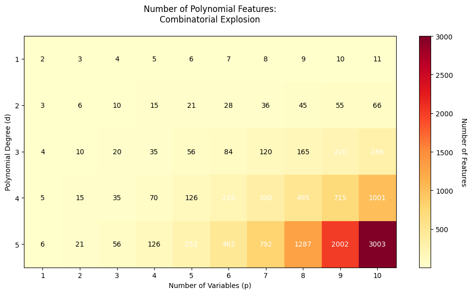
Another major concern is the curse of dimensionality when dealing with multiple features. For a dataset with features and polynomial degree , the number of terms grows as , which can quickly become computationally prohibitive. For example, with just 5 features and degree 3, you'd have 56 terms to estimate, making the model both computationally expensive and prone to overfitting.
The combinatorial growth of polynomial features can be dramatic. With 10 features and degree 4, you'd have terms. This is why polynomial regression is typically limited to low degrees (2-3) and relatively few input features in practice.
Additionally, polynomial regression can suffer from numerical instability, particularly with higher degrees. The powers of variables can become very large, leading to ill-conditioned matrices that are difficult to invert accurately. This is especially problematic when you don't properly scale features, as the magnitude differences between and can cause significant numerical issues.
Formula
The polynomial regression model extends linear regression by including polynomial terms of the independent variable. For a single variable , the polynomial regression model of degree is:
where:
- is the dependent variable (response variable we want to predict)
- is the independent variable (predictor or feature)
- is the intercept (the value of when )
- are the regression coefficients for the polynomial terms
- is the error term (random noise, assumed to be normally distributed with mean 0 and constant variance )
- is the degree of the polynomial (the highest power of in the model)
Matrix Notation
The polynomial regression model can be written in matrix form as:
where:
-
is the vector of response values (observed outcomes)
-
is the design matrix containing polynomial features up to degree
-
is the vector of coefficients to be estimated
-
is the vector of error terms (assumed to be i.i.d. with mean 0 and constant variance )
Multiple Variables
When you have more than one independent variable (feature), polynomial regression expands to include not just powers of each variable, but also all possible products (interactions) between variables up to the chosen degree. This allows the model to capture much more complex relationships between your predictors and the response.
Suppose you have independent variables: . The general form of a polynomial regression model of degree is:
where:
- is the response variable
- is the number of predictor variables
- is the -th predictor variable
- is the intercept term
- are coefficients for linear terms
- are coefficients for quadratic terms and two-way interactions
- are coefficients for cubic terms and three-way interactions
- is the error term
Let's break down what this means:
- Linear terms: Each variable appears by itself, just like in standard linear regression. For example, , , ..., .
- Quadratic terms: These include both squared terms (like , ) and products of two different variables (like ). The coefficients for these are for squares and for interactions where .
- Cubic and higher-order terms: These are all possible products of three or more variables, such as , , etc., up to the chosen degree .
- Interaction terms: Any term that involves the product of two or more different variables (e.g., ) is called an interaction term. These allow the effect of one variable to depend on the value of another.
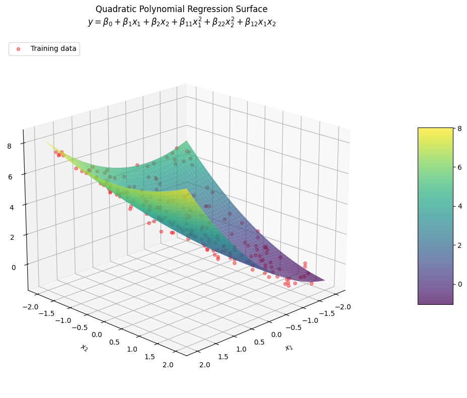
Example: Two Variables, Degree 2
If you have two variables ( and ) and use a quadratic (degree 2) polynomial, your model will look like:
where:
- is the intercept
- and are coefficients for the linear terms and
- and are coefficients for the squared terms and
- is the coefficient for the interaction term
- is the error term
Here, you have a total of 6 terms (including the intercept):
- Two linear terms: ,
- Two quadratic (squared) terms: ,
- One interaction term:
General Structure
In general, for variables and degree , the number of terms in the model (including the intercept) is given by the binomial coefficient:
where:
- is the number of predictor variables
- is the polynomial degree
- is the binomial coefficient (also written as "p+d choose d")
- The formula counts all possible combinations of variables multiplied together up to degree , including the intercept
For example, with variables and degree: terms (which matches our example above: intercept, , , , , ).
This rapid combinatorial growth is why polynomial regression with multiple variables can quickly become computationally expensive and prone to overfitting.
Summary Table of Terms
| Degree | Example Terms (for , ) | Description |
|---|---|---|
| 1 | , | Linear |
| 2 | , , | Quadratic & Interactions |
| 3 | , , , | Cubic & Higher Interactions |
In Summary, with multiple variables, polynomial regression models include all combinations of variables multiplied together up to the specified degree. This flexibility allows you to model complex, non-linear relationships, but it also means the number of terms can grow very quickly as you add more variables or increase the degree.
Mathematical Properties
The polynomial regression model maintains several important mathematical properties from linear regression. You can estimate the coefficients using the least squares method, which minimizes the sum of squared residuals:
where:
- is the residual sum of squares (the objective function to minimize)
- is the observed response value for observation
- is the predicted response value for observation
- is the number of observations
- is the polynomial degree
- is the coefficient for the -th power term
- is the predictor value for observation
The solution to this minimization problem is given by the normal equation:
where:
- is the vector of estimated coefficients
- is the transpose of the design matrix
- is the inverse of the Gram matrix
- is the vector of observed response values
The model maintains the Gauss-Markov theorem properties when the error terms satisfy the standard assumptions (zero mean, constant variance, and uncorrelated errors), making the least squares estimator the best linear unbiased estimator (BLUE).
The matrix calculations shown in the example above are simplified for educational purposes. In practice, with larger datasets or higher polynomial degrees, the matrix inversion can become numerically unstable. Modern implementations use more robust numerical methods like QR decomposition or singular value decomposition (SVD) to solve the least squares problem.
Visualizing Polynomial Regression
Let's explore how polynomial regression can capture different types of non-linear relationships through a visualization.
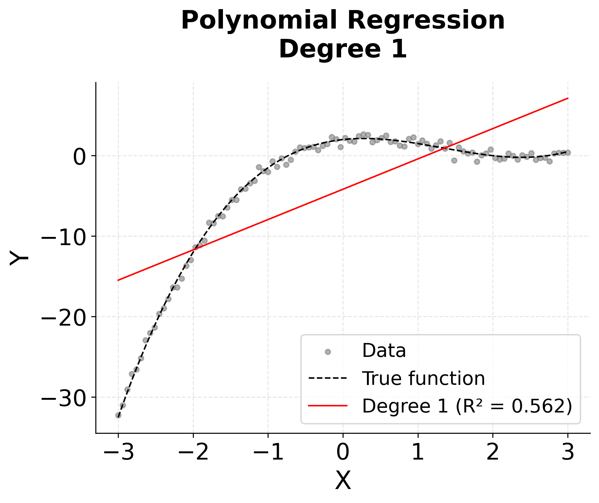
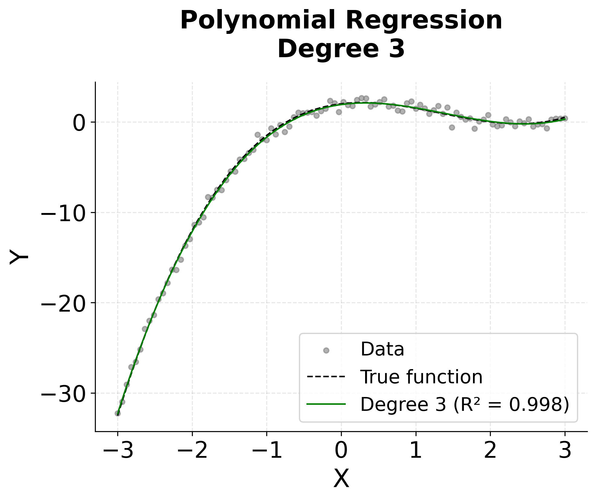
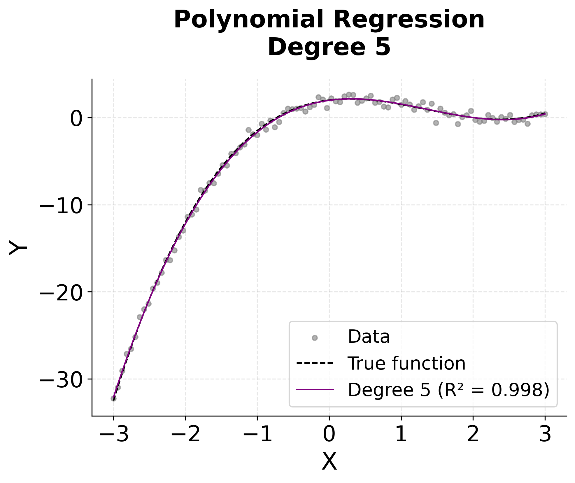
The visualization above shows how different polynomial degrees capture the underlying non-linear relationship. We can see that:
- Degree 1 (Linear): Captures only the general trend but misses the curvature
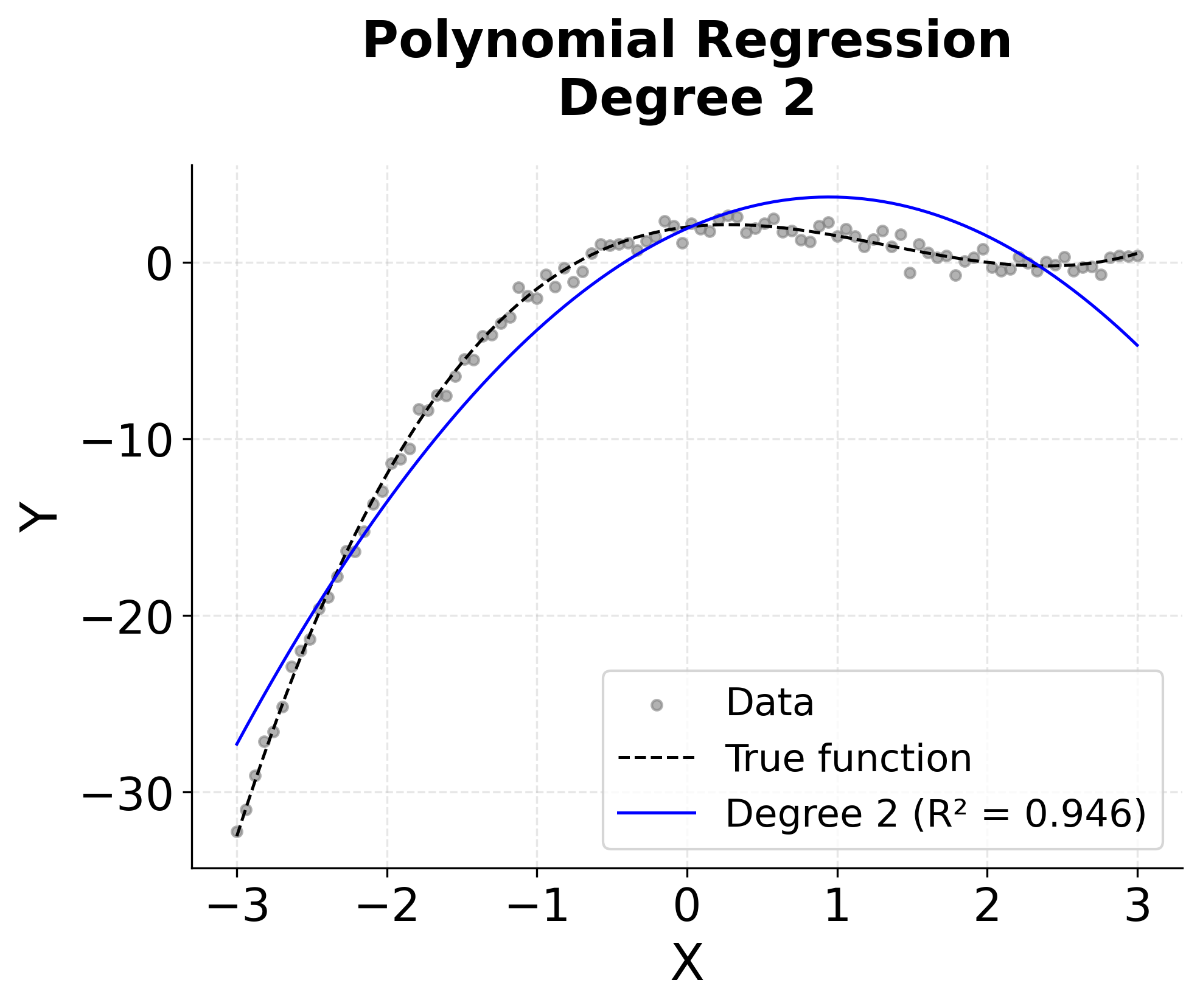
- Degree 2 (Quadratic): Begins to capture some curvature but still oversimplifies
- Degree 3 (Cubic): Closely matches the true cubic relationship
- Degree 5: Overfits the data, creating unnecessary complexity and wiggles
This illustrates the fundamental trade-off in polynomial regression: higher degrees can capture more complex relationships but risk overfitting to noise in the data.
This demonstrates the classic bias-variance trade-off in machine learning. Lower-degree polynomials have high bias (underfitting) but low variance, while higher-degree polynomials have low bias but high variance (overfitting). The optimal degree typically lies somewhere in between, where the model captures the true underlying pattern without fitting to noise.
Example
Let's work through a concrete example to understand how polynomial regression works step-by-step. You'll use a simple dataset and see the complete calculation process.
Step 1: Data Preparation
Consider the following dataset with 5 observations:
| Observation | X | Y |
|---|---|---|
| 1 | 1 | 2.1 |
| 2 | 2 | 3.9 |
| 3 | 3 | 8.1 |
| 4 | 4 | 15.9 |
| 5 | 5 | 25.1 |
Step 2: Setting Up the Quadratic Model
We'll fit a quadratic polynomial regression model:
Step 3: Constructing the Design Matrix
For a quadratic model, our design matrix includes columns for the intercept, , and :
Step 4: Matrix Calculations
The response vector is:
Now you calculate (the Gram matrix). First, note that is the transpose of :
For example, the element in row 1, column 2 is: .
Similarly, calculate :
For example, the first element is: .
Step 5: Solving for Coefficients
Using the normal equation , we first compute the inverse of :
Therefore, the coefficient estimates are:
where:
- is the estimated intercept
- is the estimated coefficient for the linear term
- is the estimated coefficient for the quadratic term
Step 6: Final Model
Our fitted quadratic polynomial regression model is:
where:
- is the predicted response value
- is the predictor variable
- The coefficients indicate a quadratic relationship with both linear and quadratic components
This model shows that the relationship has a negative linear component () and a positive quadratic component (), creating a U-shaped curve that increases more rapidly for larger values of .
Step 7: Verification
Let's verify our model by calculating predictions for each observation:
- For : (actual: 2.1, residual: )
- For : (actual: 3.9, residual: )
- For : (actual: 8.1, residual: )
- For : (actual: 15.9, residual: )
- For : (actual: 25.1, residual: )
where the residual is defined as (predicted minus actual).
The model captures the quadratic trend very well, with small residuals. The residual sum of squares is:
where:
- is the residual sum of squares
- Each term represents the squared difference between predicted and actual values
- A smaller RSS indicates a better fit to the data
This small RSS value of 0.265 indicates an excellent fit to the data.
Implementation in Scikit-learn
Scikit-learn provides excellent tools for implementing polynomial regression through the PolynomialFeatures transformer and LinearRegression estimator. Let's walk through a complete implementation that demonstrates how to build, train, and evaluate polynomial regression models.
Setting Up the Data
We'll start by generating synthetic data with a known cubic relationship, which will allow us to see how well polynomial regression can recover the true underlying function.
The data follows a cubic polynomial with added Gaussian noise. By splitting into training (70%) and test (30%) sets, we can evaluate how well the model generalizes to unseen data.
Building a Polynomial Regression Pipeline
The most efficient way to implement polynomial regression in scikit-learn is using a Pipeline that combines the PolynomialFeatures transformer with LinearRegression. This ensures that the same polynomial transformation is consistently applied to both training and test data.
The low MSE and high R² score (close to 1.0) indicate excellent model performance. Since our data was generated from a cubic function and we used a degree-3 polynomial, the model successfully captures the true underlying relationship. The R² score tells us that the model explains nearly all the variance in the test data.
The coefficients show the contribution of each polynomial term. Comparing these to our true function (), we can see the model has successfully recovered values close to the true parameters, despite the added noise.
Comparing Different Polynomial Degrees
A critical question in polynomial regression is choosing the right degree. Let's compare models with different degrees to understand the bias-variance trade-off.
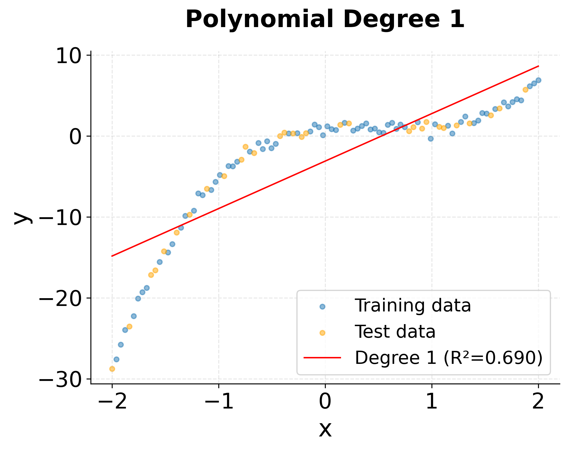
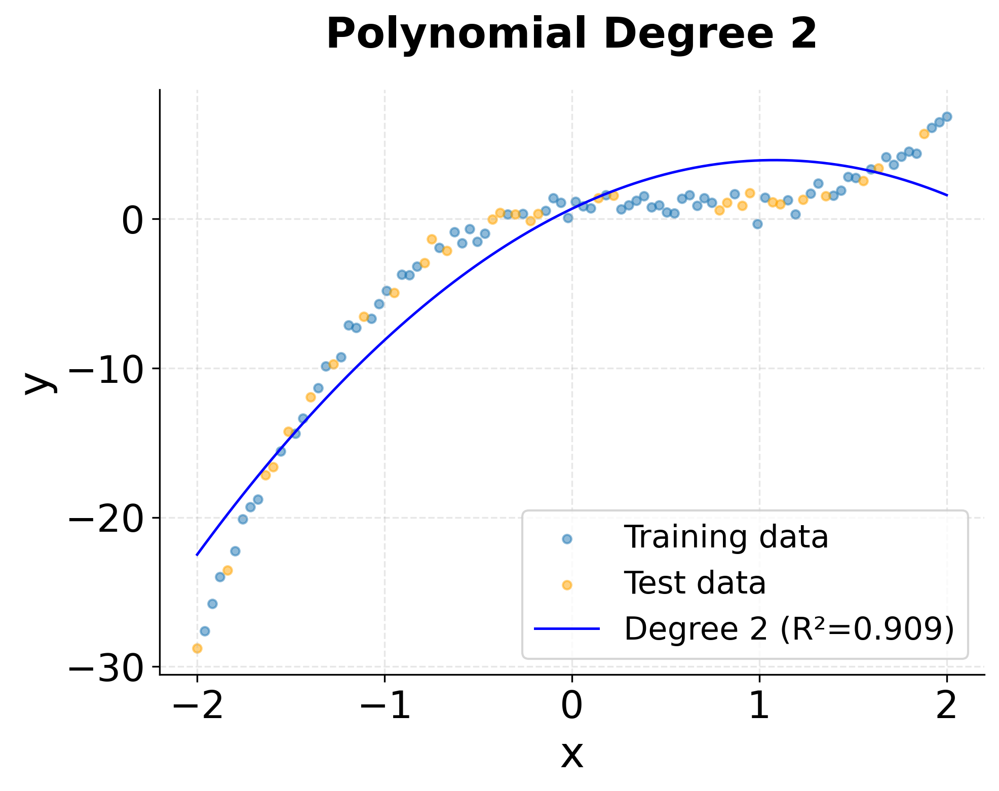
The comparison reveals important insights about model selection:
- Degree 1 (Linear): High MSE and low R² indicate underfitting. A straight line cannot capture the cubic relationship.
- Degree 2 (Quadratic): Improved performance but still underfits the true cubic function.
- Degree 3 (Cubic): Optimal performance with the lowest MSE. This matches the true data-generating process.
- Degrees 4-5: Similar or slightly worse performance than degree 3, suggesting potential overfitting to noise in the training data.
The degree-3 model achieves the best balance between bias and variance, as expected since the true relationship is cubic. Higher degrees don't improve performance and risk overfitting, especially with limited training data.
Visualizing Model Predictions
Let's visualize how different polynomial degrees fit the data to better understand their behavior.
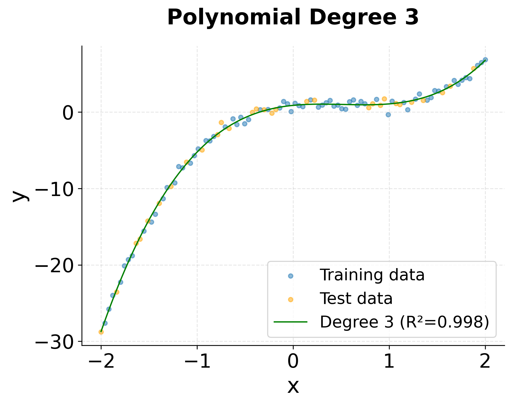
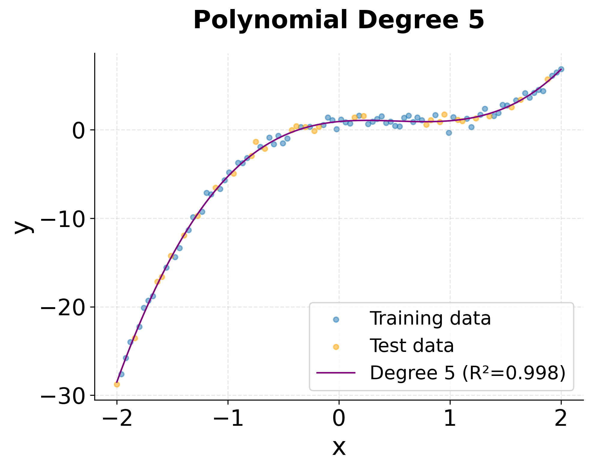
The visualizations clearly show the progression from underfitting (degree 1) to optimal fit (degree 3) to potential overfitting (degree 5). The degree-3 model smoothly captures the underlying cubic trend, while the degree-5 model shows slight oscillations that fit noise rather than the true pattern.
Key Parameters
Below are the main parameters that control polynomial regression behavior and performance.
PolynomialFeatures Parameters:
degree: The maximum degree of polynomial features to generate (default: 2). This is the most critical parameter. Start with low values (2-3) and increase only if needed. Higher degrees capture more complex patterns but risk overfitting.include_bias: Whether to include the intercept column of ones (default: True). Typically set toTruewhen using withLinearRegression, which expects the bias term in the feature matrix.interaction_only: IfTrue, only interaction features are produced, not powers (default: False). Use this when you want to model interactions between variables without including squared or higher-power terms.
LinearRegression Parameters:
fit_intercept: Whether to calculate the intercept (default: True). When usingPolynomialFeatureswithinclude_bias=True, this is typically set toFalseto avoid redundancy, though scikit-learn handles this automatically.copy_X: Whether to copy the input data (default: True). Set toFalseto save memory if you don't need the original data preserved.
Pipeline Benefits:
- Automatically applies the same polynomial transformation to training and test data
- Simplifies cross-validation and hyperparameter tuning
- Ensures reproducible preprocessing steps
- Makes code more maintainable and less error-prone
Key Methods
The following methods are used to train and apply polynomial regression models.
fit(X, y): Trains the polynomial regression model on input features X and target values y. This applies the polynomial transformation and fits the linear regression coefficients.predict(X): Returns predicted values for input data X. The polynomial transformation is automatically applied before making predictions.score(X, y): Returns the R² score (coefficient of determination) on the given test data. Values closer to 1.0 indicate better fit.get_params(): Returns the parameters of the pipeline components. Useful for inspecting or modifying the model configuration.set_params(**params): Sets the parameters of the pipeline. Commonly used with grid search for hyperparameter tuning.
Practical Applications
When to Use Polynomial Regression
Polynomial regression is particularly effective when you have continuous target variables and suspect non-linear relationships that can be approximated with smooth polynomial curves. The method excels in engineering applications where physical relationships often follow polynomial patterns, such as modeling stress-strain curves in materials science, temperature effects on material properties, or fluid dynamics problems. These domains benefit from polynomial regression because the underlying physics often produces smooth, continuous relationships that can be well-represented by polynomial functions of moderate degree.
In economics and finance, polynomial regression proves valuable for modeling relationships with natural curvature, such as the risk-return trade-off in portfolio optimization or the relationship between advertising spend and sales revenue. Marketing analysts frequently use quadratic or cubic polynomials to capture diminishing returns, where initial investments yield strong results but additional spending produces progressively smaller gains. The method is also useful in dose-response studies in pharmacology, where the effect of a drug often follows a non-linear but smooth relationship with dosage.
The approach works best when you have moderate amounts of data (hundreds to thousands of observations) and when the underlying relationship is genuinely smooth rather than highly irregular or discontinuous. Polynomial regression is less suitable for problems with sharp transitions, categorical relationships, or highly complex patterns that would require very high-degree polynomials. In such cases, methods like decision trees, splines, or neural networks may be more appropriate. The key advantage of polynomial regression is its balance between flexibility and interpretability—it can model non-linear relationships while maintaining the familiar statistical framework and diagnostic tools of linear regression.
Best Practices
To achieve optimal results with polynomial regression, begin by selecting an appropriate polynomial degree through systematic cross-validation rather than visual inspection alone. Start with low degrees (typically 2 or 3) and incrementally increase while monitoring both training and validation performance. Use k-fold cross-validation with at least 5 folds to assess generalization performance, and watch for signs of overfitting where training error continues to decrease but validation error increases. The optimal degree typically occurs where validation error reaches its minimum, and you should favor simpler models when performance differences are marginal.
Feature scaling is essential before applying polynomial transformations, particularly for degrees higher than 2. Use StandardScaler to center and scale your features to unit variance, or MinMaxScaler if you need features in a specific range. Apply scaling before generating polynomial features to prevent numerical instability that arises when features like have vastly different magnitudes than . When working with multiple input variables, be mindful of the combinatorial explosion in feature count—with 5 variables and degree 3, you generate 56 features. In such cases, consider using interaction_only=True in PolynomialFeatures to include only interaction terms without higher powers, or apply regularization techniques like Ridge or Lasso to manage the increased model complexity.
Always use pipelines to ensure consistent preprocessing between training and prediction. A pipeline that combines StandardScaler, PolynomialFeatures, and LinearRegression guarantees that test data receives identical transformations as training data, preventing subtle bugs and ensuring reproducibility. Set random_state parameters for reproducibility, and evaluate your model using multiple metrics—R² score for overall fit, mean squared error for prediction accuracy, and residual plots to check for patterns that might indicate model misspecification. When comparing models of different degrees, consider both statistical measures and domain knowledge to ensure your chosen model makes practical sense for your application.
Data Requirements and Preprocessing
Polynomial regression requires continuous numerical features and a continuous target variable. The method assumes that relationships between variables are smooth and differentiable, making it unsuitable for categorical predictors without proper encoding or for target variables with discrete jumps. Your data should have sufficient observations relative to the number of polynomial features you plan to generate—as a general guideline, aim for at least 10-20 observations per feature to avoid overfitting. With degree 3 polynomials on a single variable (4 features including intercept), this means at least 40-80 observations, though more is always preferable.
Missing values must be handled before applying polynomial regression, as the method cannot work with incomplete data. Imputation strategies depend on your domain—mean or median imputation works for data missing at random, while more sophisticated approaches like K-nearest neighbors imputation may be appropriate for structured missingness patterns. Outliers can have disproportionate influence on polynomial regression, especially with higher degrees, since polynomial terms amplify extreme values. Examine your data for outliers using box plots or z-scores, and consider whether they represent genuine extreme observations or data quality issues. If outliers are legitimate, robust regression techniques or data transformations may help reduce their influence.
The distribution of your predictor variables affects polynomial regression performance. Ideally, predictors should have reasonable coverage across their range without large gaps, as polynomials can behave erratically when extrapolating beyond the training data range. If your data is heavily skewed, consider log or square root transformations before generating polynomial features, as these can stabilize variance and improve model fit. However, be cautious with transformations, as they change the interpretation of coefficients and may complicate communication of results to non-technical stakeholders.
Common Pitfalls
One of the most frequent mistakes is choosing polynomial degree based solely on training performance or visual fit without proper validation. This often leads to overfitting, where the model captures noise rather than true underlying patterns. High-degree polynomials can fit training data nearly perfectly while performing poorly on new data, especially near the boundaries of the data range where polynomial curves can exhibit wild oscillations. Always use cross-validation to select the degree, and be skeptical of models that require degrees higher than 4 or 5—such complexity often indicates that polynomial regression may not be the right approach for your problem.
Failing to scale features before polynomial transformation is another common error that can cause numerical instability and poor convergence. When you raise unscaled features to high powers, the resulting values can become extremely large or small, leading to overflow errors or ill-conditioned matrices that are difficult to invert accurately. This problem becomes more severe with higher degrees and can produce unreliable coefficient estimates even when the algorithm appears to converge. The solution is straightforward: always apply feature scaling before polynomial feature generation, and use pipelines to ensure this preprocessing happens consistently.
A subtler pitfall involves using polynomial regression with multiple correlated predictors, which can lead to severe multicollinearity when interaction terms are included. For example, if and are highly correlated, their polynomial terms like , , and will be even more correlated, making coefficient estimates unstable and difficult to interpret. In such cases, consider regularization methods like Ridge regression, which can handle multicollinearity more gracefully, or use principal component analysis to decorrelate your features before applying polynomial transformations. Finally, avoid the temptation to extrapolate far beyond your training data range—polynomial models often behave unpredictably outside the region where they were fitted, and predictions in these regions should be treated with considerable skepticism.
Computational Considerations
Polynomial regression has computational complexity that depends primarily on the number of polynomial features rather than the polynomial degree itself. For a dataset with observations and input features at degree , the number of polynomial features grows as , and the computational cost of fitting scales as where is the number of features. For small to moderate feature counts (up to a few dozen features), this is quite manageable on modern hardware. However, with 10 input features at degree 4, you generate 1,001 polynomial features, making the problem substantially more expensive.
For datasets with fewer than 10,000 observations and moderate feature counts (under 50 polynomial features), polynomial regression typically runs in seconds on standard hardware. Memory requirements are generally modest, as you only need to store the design matrix and intermediate calculations. However, with very large datasets (millions of observations) or high-dimensional feature spaces (hundreds of polynomial features), memory can become a constraint. In such cases, consider using mini-batch or online learning approaches, though these are less common for polynomial regression than for other methods. Alternatively, reduce dimensionality by selecting only the most important input features or using lower polynomial degrees.
When working with multiple input variables, the combinatorial explosion in feature count can make polynomial regression impractical beyond degree 3 or 4. For 20 input features at degree 3, you would generate 1,771 polynomial features, requiring substantial memory and computation time. In these scenarios, consider alternative approaches such as generalized additive models (GAMs) that model non-linear effects for each variable separately, or use feature selection to identify the most important variables before applying polynomial transformations. Sparse polynomial regression, which selects only relevant polynomial terms, can also help manage complexity in high-dimensional settings.
Performance Evaluation and Deployment
Evaluating polynomial regression performance requires attention to both statistical metrics and practical considerations. The R² score provides a measure of overall fit, with values above 0.7 generally indicating good predictive power, though acceptable thresholds vary by domain. However, R² alone can be misleading with polynomial regression, as it always increases with polynomial degree on training data. Instead, focus on cross-validated R² or adjusted R², which penalizes model complexity. Mean squared error (MSE) and root mean squared error (RMSE) provide interpretable measures of prediction accuracy in the original units of your target variable, making them valuable for communicating model performance to stakeholders.
Residual analysis is particularly important for polynomial regression. Plot residuals against predicted values to check for patterns—residuals should appear randomly scattered around zero without systematic trends. Patterns in residual plots often indicate that your chosen polynomial degree is too low (underfitting) or that important variables are missing from the model. Also examine residuals across the range of predictor variables to ensure the model fits well throughout the data range, not just in the center. Polynomial models sometimes fit poorly near the boundaries of the data, where polynomial curves can exhibit unexpected behavior.
When deploying polynomial regression models, ensure that your production pipeline includes all preprocessing steps in the correct order: feature scaling, polynomial transformation, and prediction. Using scikit-learn pipelines simplifies deployment by encapsulating all transformations in a single object that can be serialized and loaded in production environments. Monitor model performance over time, as polynomial models can degrade if the data distribution shifts or if predictions are needed outside the original training range. For real-time applications, polynomial regression offers fast prediction times since it only requires matrix multiplication, making it suitable for latency-sensitive deployments. However, be cautious about extrapolation—if production data extends beyond training ranges, consider retraining the model or implementing safeguards that flag out-of-range predictions for manual review.
Summary
Polynomial regression serves as a powerful bridge between simple linear regression and more complex non-linear modeling techniques. By extending the linear regression framework to include polynomial terms, it allows you to capture curved relationships while maintaining the interpretability and statistical rigor of linear models. The method is particularly valuable when you're dealing with smooth, continuous relationships that can be approximated by polynomial curves.
Successful polynomial regression requires careful model selection and validation. While the technique can capture complex non-linear patterns, it's susceptible to overfitting, especially with higher degrees. Balancing model complexity with generalization performance through cross-validation helps select appropriate polynomial degrees while monitoring for signs of overfitting. The computational efficiency and interpretability of polynomial regression make it an excellent choice for many practical applications, particularly in domains where understanding the relationship between variables is as important as prediction accuracy.
When you implement it thoughtfully with proper preprocessing, feature scaling, and model validation, polynomial regression provides a robust and interpretable approach to modeling non-linear relationships. It serves as an essential tool in your data science toolkit, offering a stepping stone to more advanced techniques while maintaining the analytical transparency that makes linear regression so valuable in practice.
Quiz
Ready to test your understanding of polynomial regression? Take this quiz to reinforce what you've learned about modeling non-linear relationships with polynomial terms.

Comments