

Master option Greeks: delta, gamma, theta, vega, and rho. Learn sensitivity analysis, delta hedging, and portfolio risk management techniques.
Choose your expertise level to adjust how many terms are explained. Beginners see more tooltips, experts see fewer to maintain reading flow. Hover over underlined terms for instant definitions.
The Greeks and Option Risk Management
In the previous chapter, we derived the Black-Scholes formula and learned how to price European options. But pricing is only half the story. Once you own an option, or a portfolio of options, you face a crucial question: how will its value change as market conditions evolve? The underlying stock might move, time will pass, volatility expectations might shift, and interest rates could change. Each of these factors affects your position's value, often in non-linear and interacting ways.
The Greeks provide the answer. They are a collection of sensitivity measures that quantify how much an option's price will change in response to small changes in various market parameters. Named after Greek letters (with one notable exception), these risk measures form the foundation of modern option risk management. Delta tells you how the option responds to moves in the underlying asset. Gamma reveals the curvature of that response. Theta captures the relentless erosion of time value. Vega measures exposure to changes in implied volatility. Rho quantifies interest rate sensitivity.
Understanding the Greeks transforms you from a passive option holder into an active risk manager. You don't simply buy options and hope for the best. You construct portfolios with specific Greek exposures, dynamically hedge away unwanted risks, and profit from the risks you choose to retain. You might maintain a delta-neutral book while harvesting theta. You might build positions with high vega and minimal directional exposure. You might set limits on gamma to control the portfolio's sensitivity to large market moves.
This chapter develops each Greek mathematically, building on the calculus foundations from Part I and the Black-Scholes framework from the preceding chapters. We'll derive closed-form expressions for each Greek, understand their behavior across different option characteristics, and learn how you combine them to manage complex option portfolios.
Delta: Sensitivity to the Underlying Price
Delta () measures the rate of change of an option's price with respect to changes in the underlying asset's price. To understand why this matters, imagine you hold a call option and the stock price rises by one dollar. How much does your option become worth? Delta answers this question as the fundamental sensitivity measure.
Mathematically, delta is the first partial derivative of the option price with respect to the spot price:
where:
- : option delta
- : option value
- : underlying asset price
The partial derivative notation indicates that we are measuring how the option value changes when only the stock price moves, holding all other variables constant. This is a key conceptual point: delta isolates the effect of price movements from other factors like time decay or volatility changes.
Delta for European Options
Building on the Black-Scholes formula from the previous chapter, we can derive explicit formulas for delta. The Black-Scholes framework provides closed-form solutions, meaning we can write down exact expressions for these sensitivities rather than having to estimate them numerically. Recall that for a European call option:
where:
- : European call option price
- : current stock price
- : strike price
- : risk-free interest rate
- : time to expiration
- : cumulative standard normal distribution function
- : probability factor adjusting for time and volatility
- : probability factor adjusting for volatility drag
- : expected value of the asset at expiration, conditional on the option being in-the-money
- : present value of the strike price, weighted by the probability of exercise
To find delta, we need to differentiate this expression with respect to the stock price . This requires careful application of calculus because both terms depend on , and and themselves are functions of . The stock price appears explicitly in the first term and implicitly through the and terms that sit inside the cumulative normal distribution functions.
Taking the partial derivative with respect to requires applying the product and chain rules:
The first term, , comes from differentiating directly. The second and third terms arise from the chain rule: when we differentiate and , we get the standard normal probability density function evaluated at and , multiplied by the derivatives of and with respect to .
When we work through this calculation, the terms involving the derivatives of cancel out. Specifically, we can show that , and since , these terms exactly offset. These terms cancel because of the risk-neutral framework and the Black-Scholes model structure. This yields the simple result:
where:
- : delta of a European call
- : probability term acting as the hedge ratio
This formula tells us that call delta equals the cumulative normal distribution evaluated at . Since the cumulative normal distribution ranges from 0 to 1, call delta is always between 0 and 1. This bounded range has important economic meaning: a one-dollar increase in the stock price cannot possibly increase the call value by more than one dollar, because the call at best moves one-for-one with the stock when it is extremely deep in the money.
For a European put option with price , a similar derivation yields:
where:
- : delta of a European put
- : negative hedge ratio for the put
Put delta is always negative, ranging from -1 to 0. This makes intuitive sense: when the stock price rises, a put option becomes less valuable because the right to sell at a fixed strike price is worth less when the current market price is higher. The relationship is a direct consequence of put-call parity, which states that the difference between a call and put with the same strike and expiration equals the present value of a forward contract.
Interpreting Delta
Delta has several intuitive interpretations that illuminate different aspects of option behavior:
-
Hedge ratio: Delta represents the number of shares needed to hedge one option. If a call has , you need to short 0.6 shares of stock to create a delta-neutral position that is immune (to first order) to small price movements. This interpretation is crucial for you if you want to eliminate directional risk while maintaining option positions.
-
Probability proxy: For a call option, delta roughly approximates the risk-neutral probability that the option will expire in-the-money. A deep in-the-money call with is almost certain to be exercised, while a far out-of-the-money call with is unlikely to finish in-the-money. Note that this refers to risk-neutral probability, not real-world probability. However, it still provides intuition on the likelihood of the option expiring in-the-money.
-
Dollar sensitivity: If you own one call option and , then a $1 increase in the stock price will increase your option value by approximately $0.60. This direct translation of delta into dollar terms makes it immediately useful for risk assessment. You often think in terms of "delta dollars," which is delta multiplied by the notional value of the position.
Delta Behavior
Delta exhibits characteristic behavior depending on moneyness and time to expiration. Understanding these patterns is essential for you when trading options, as they reveal how your exposure changes as market conditions evolve. To visualize this, we first define a Python function for delta that handles both calls and puts, as well as the expiration boundary condition:
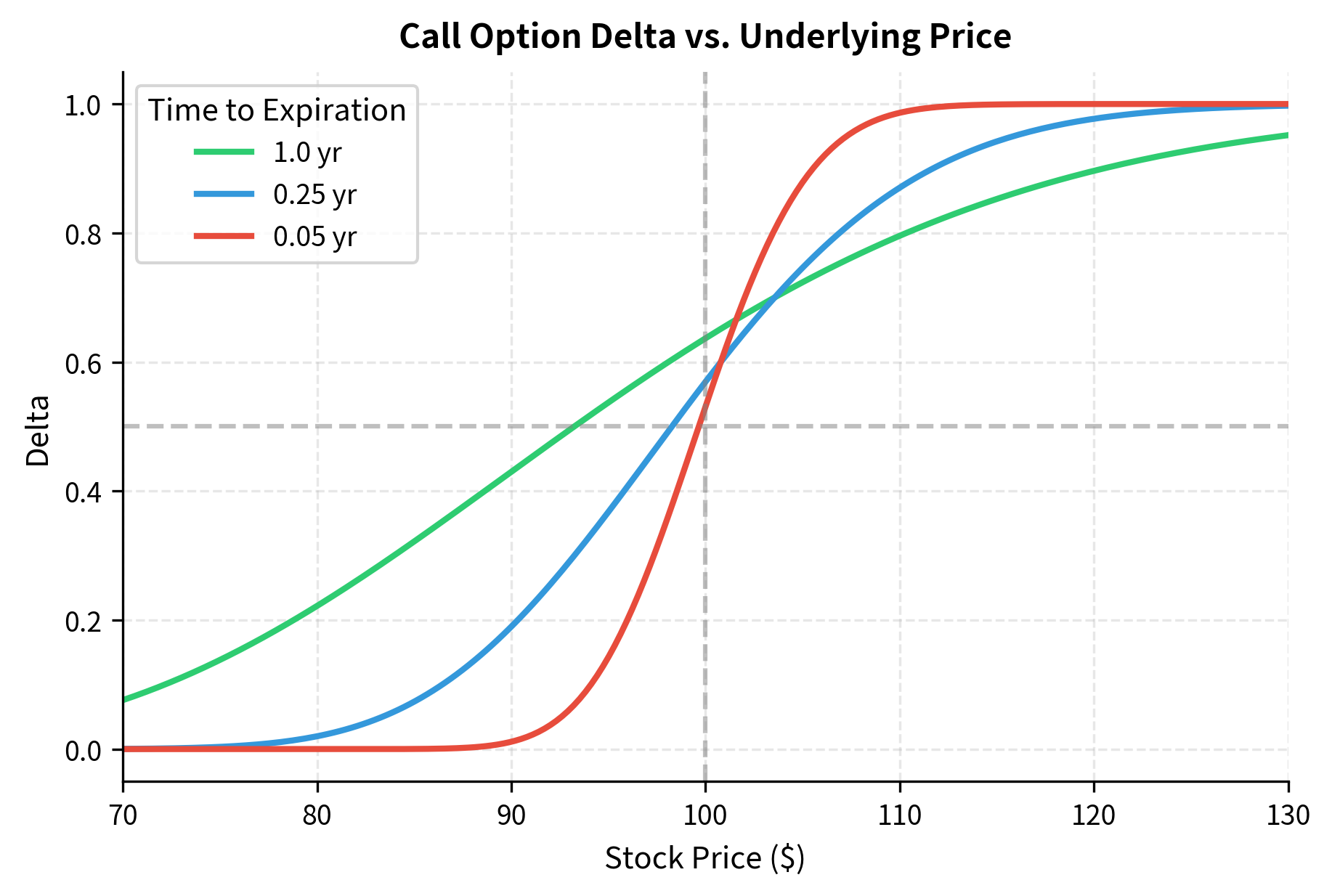
The figure reveals several important patterns. For at-the-money options, delta is approximately 0.5, meaning the option moves roughly half as much as the underlying stock. As the option moves deeper in-the-money, delta approaches 1 for calls (or -1 for puts), because the option increasingly behaves like the underlying stock itself. Out-of-the-money options have deltas approaching 0 because they are unlikely to have any value at expiration. Near expiration, the delta curve steepens dramatically, creating a step function around the strike price. This steepening reflects the increasing certainty about whether the option will expire in or out of the money: with little time remaining, small price movements can definitively determine the option's fate.

The comparison of call and put deltas visually confirms the put-call parity relationship. The vertical distance between the two curves is exactly one at every stock price, illustrating that . This relationship holds because put-call parity states , and differentiating both sides with respect to gives .
Gamma: The Curvature of Delta
Gamma () measures the rate of change of delta with respect to changes in the underlying price. While delta tells you your current exposure to price movements, gamma tells you how that exposure will change as the price moves. This second-order sensitivity captures the essence of what makes options non-linear instruments, fundamentally different from stocks or forward contracts.
Mathematically, gamma is the second partial derivative of the option price with respect to the spot price:
where:
- : option gamma
- : option value
- : underlying asset price
- : option delta
The equivalence between these two expressions follows directly from the definition: since delta is the first derivative of price with respect to spot, gamma is the derivative of delta, which is the second derivative of price. Gamma tells you how quickly your hedge (delta) will become stale as the underlying moves. A high gamma position requires frequent rebalancing to maintain delta neutrality.
Gamma for European Options
Using the Black-Scholes framework, we derive gamma by differentiating delta with respect to the spot price . Recall that for a call, . To find gamma, we differentiate this expression with respect to the stock price:
The chain rule tells us to multiply the derivative of the outer function (the cumulative normal, whose derivative is the standard normal PDF) by the derivative of the inner function ( with respect to ). The derivative comes from recognizing that contains , and the derivative of the natural logarithm of is .
This leads to the standard formula:
where:
- : option gamma
- : standard normal probability density function
- : underlying price
- : strike price
- : risk-free interest rate
- : volatility
- : time to expiration
- : standardized moneyness factor
Calls and puts have identical gamma because of put-call parity. Since is linear in , the second derivatives are equal. This makes intuitive sense: both calls and puts exhibit the same curvature in their payoff profiles; they simply face different directions.
Understanding Gamma
Gamma captures the convexity or curvature in an option's value as a function of the underlying price. This curvature is what makes options fundamentally different from linear instruments like forwards. A forward contract has constant delta (equal to one) and zero gamma: its value moves one-for-one with the underlying at all prices. An option, by contrast, has variable delta that changes with the stock price, and this variability is measured by gamma.
Positive gamma means you benefit from large moves in either direction. If you're long an option (long gamma), your delta increases as the stock rises and decreases as the stock falls. You automatically become more long when prices rise and more short when prices fall. This convexity is what you pay for through theta (time decay).
Consider a delta-neutral portfolio. If gamma is positive, a large move in either direction benefits the position; the portfolio gains value whether the stock jumps up or crashes down. This is why being "long gamma" is attractive but costly: you pay time decay for the privilege of this favorable convexity. Conversely, being "short gamma" means you earn time decay but face unlimited downside if the market makes a large move. If you sell options, you are typically short gamma and must actively manage this exposure.
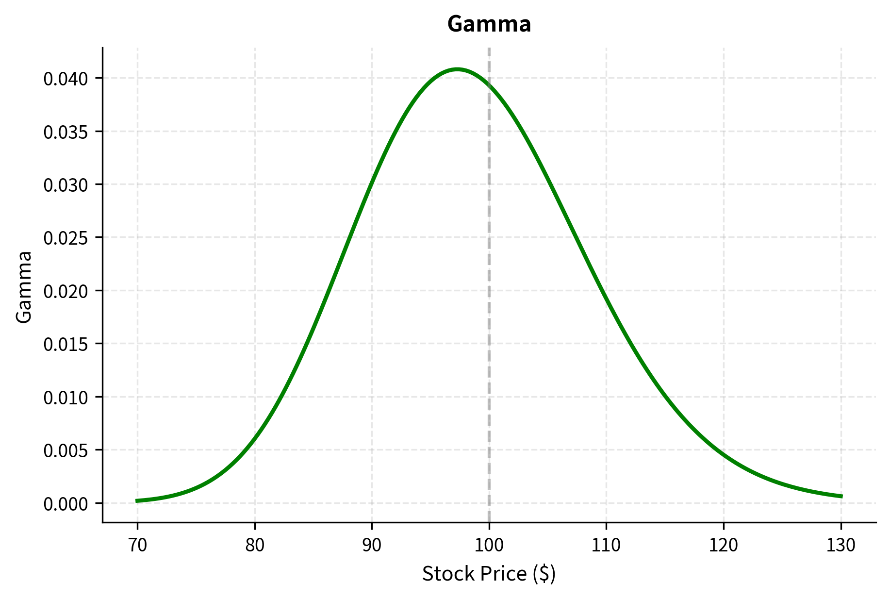
Gamma Behavior
We implement the gamma calculation below. Note that the formula is the same for calls and puts, so we do not need an option type argument:
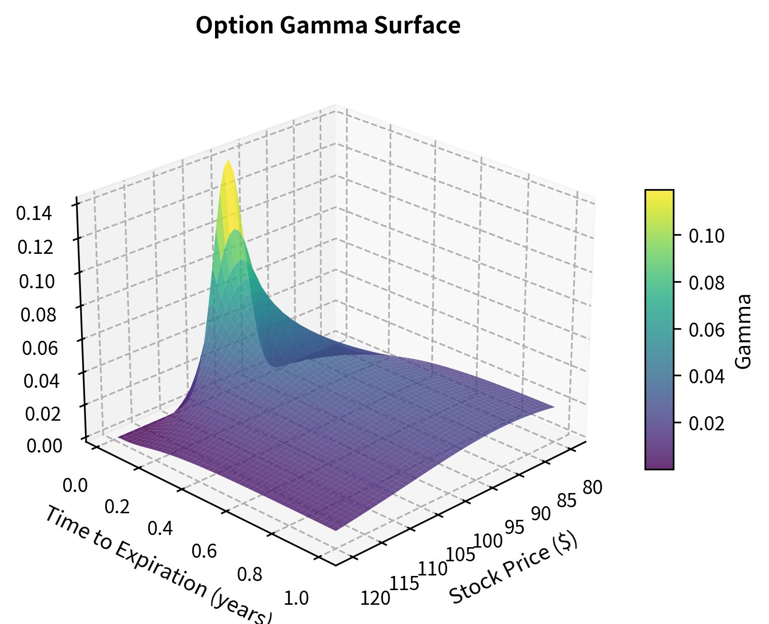
Gamma has distinctive characteristics that become clear when we examine the three-dimensional surface:
-
Maximum at-the-money: Gamma is highest when the option is at-the-money because that's where delta is most sensitive to price changes. At the money, the option is on the knife's edge between having value and being worthless, so small price movements can dramatically change its prospects.
-
Increases near expiration: As time passes, gamma for ATM options increases dramatically. This creates "gamma risk" for short positions near expiration. With little time remaining, even small moves in the underlying can cause large changes in delta, requiring urgent and potentially costly rebalancing.
-
Approaches zero OTM and ITM: Deep out-of-the-money and deep in-the-money options have low gamma because their deltas are already near their extreme values (0 or ±1) and don't change much. An option that is certain to be exercised or certain to expire worthless has stable delta.
Theta: Time Decay
Theta () measures the rate of change of an option's price with respect to the passage of time. Unlike the other Greeks, which measure sensitivities to variables that can move up or down, time moves in only one direction: forward. Every day that passes brings the option closer to expiration, and for most options, this passage of time erodes value. This erosion is called time decay, and theta quantifies its rate.
Mathematically, theta is defined as:
where:
- : option theta
- : option value
- : time
Note: In practice, theta is often expressed as the negative of this derivative, representing the loss in option value per day, since we typically think of time decay as a cost. You might say "my theta is negative twenty dollars," meaning the position loses twenty dollars per day to time decay alone.
Theta for European Options
Theta is more complex to derive than delta or gamma because time appears in several places: the discount factor, volatility scaling, and the and terms. The resulting formulas have two distinct components that reflect different economic effects.
For a European call option:
where:
- : theta of a European call
- : underlying price
- : standard normal probability density function
- : volatility
- : time to expiration
- : risk-free interest rate
- : strike price
- : cumulative standard normal distribution value
- : probability factor adjusting for time and volatility
- : probability factor adjusting for volatility drag
- First term: pure time value decay (gamma cost)
- Second term: interest on strike price (time value of money)
The first term in the theta formula represents the pure decay of the option's time value. This term is always negative because the factor involves only positive quantities arranged to produce a negative result. This pure time decay reflects the loss of optionality: with less time remaining, there is less opportunity for favorable price movements. The second term reflects the time value of money: as expiration approaches, the present value of the strike price increases (since it is discounted over a shorter period), which reduces call value.
For a European put option:
where:
- : theta of a European put
- : underlying price
- : volatility
- : time to expiration
- : risk-free interest rate
- : strike price
- : standard normal probability density function
- : cumulative standard normal distribution value
- First term: same volatility decay as the call
- Second term: interest benefit from delaying strike payment
These formulas decompose into two components: the first term represents the pure time value decay (always negative for long positions), while the second term reflects the time value of money effect on the discounted strike price. For puts, this second term is positive because the put holder benefits from delaying receipt of the strike price (which earns interest in the meantime).
The Theta-Gamma Trade-off
A fundamental relationship connects theta and gamma. From the Black-Scholes PDE, for a delta-hedged portfolio:
where:
- : time decay
- : curvature risk
- : volatility
- : stock price
- : option delta
- : risk-free rate
- : option value
This equation, which comes directly from the Black-Scholes partial differential equation, establishes that theta and gamma are two sides of the same coin. For a delta-neutral position (where offsets the directional exposure), the right-hand side is approximately , which is small for typical option values and interest rates. This means that for a delta-neutral position, theta and gamma are inversely related. If you're long gamma (benefiting from moves), you're paying theta. If you're short gamma (hurt by moves), you're earning theta. This trade-off is at the heart of many options strategies.
The intuition is straightforward: gamma represents the benefit you receive from large price movements, while theta represents the cost of holding that beneficial position. The market prices options so that, on average, the expected benefit from gamma equals the expected cost of theta. This is why you cannot get something for nothing in options markets: the advantages of positive gamma come at a price.
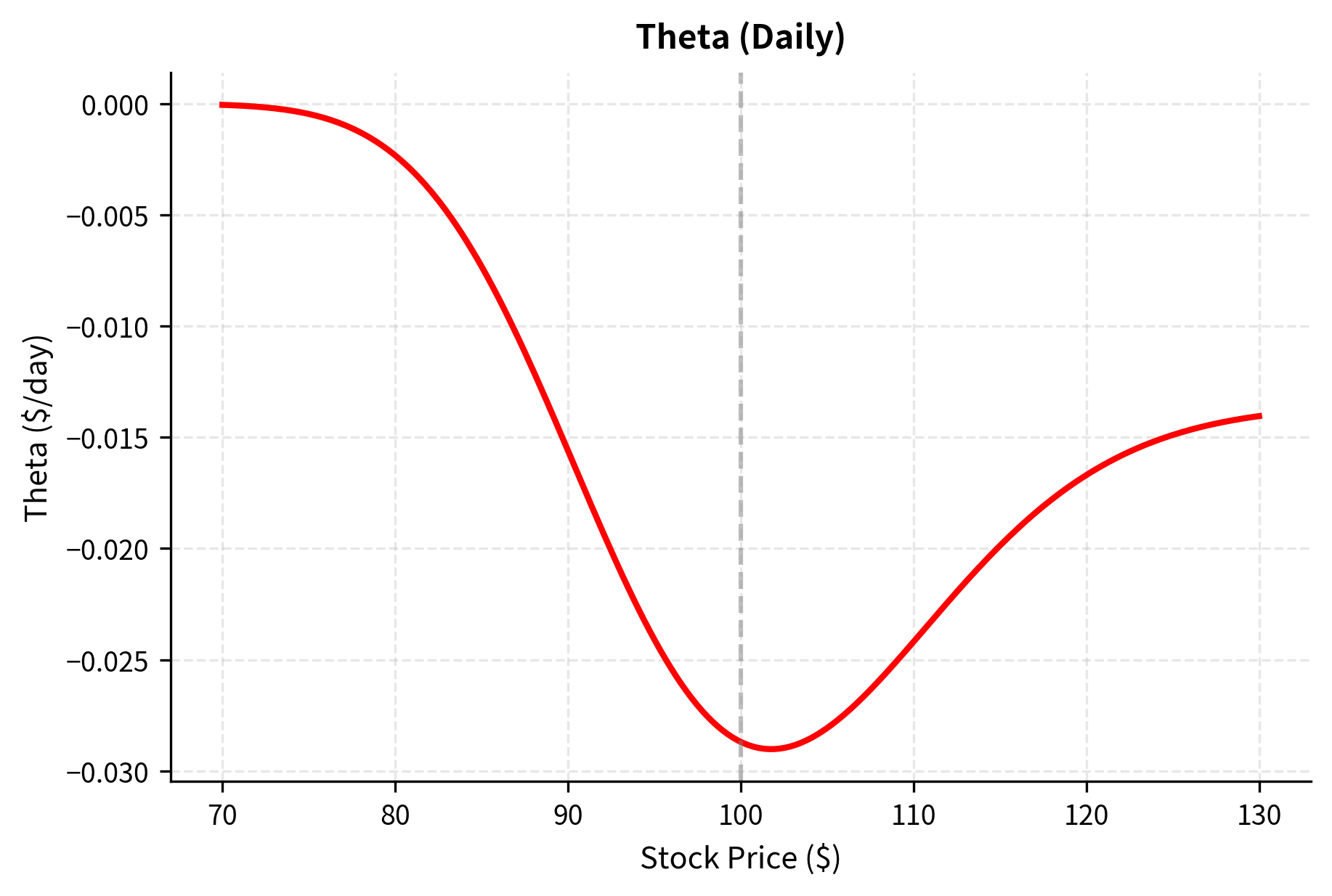
The implementation of theta requires careful handling of the two terms: the time decay of the volatility component and the interest rate component. We also convert the result to a daily decay figure in the plotting step for easier interpretation:
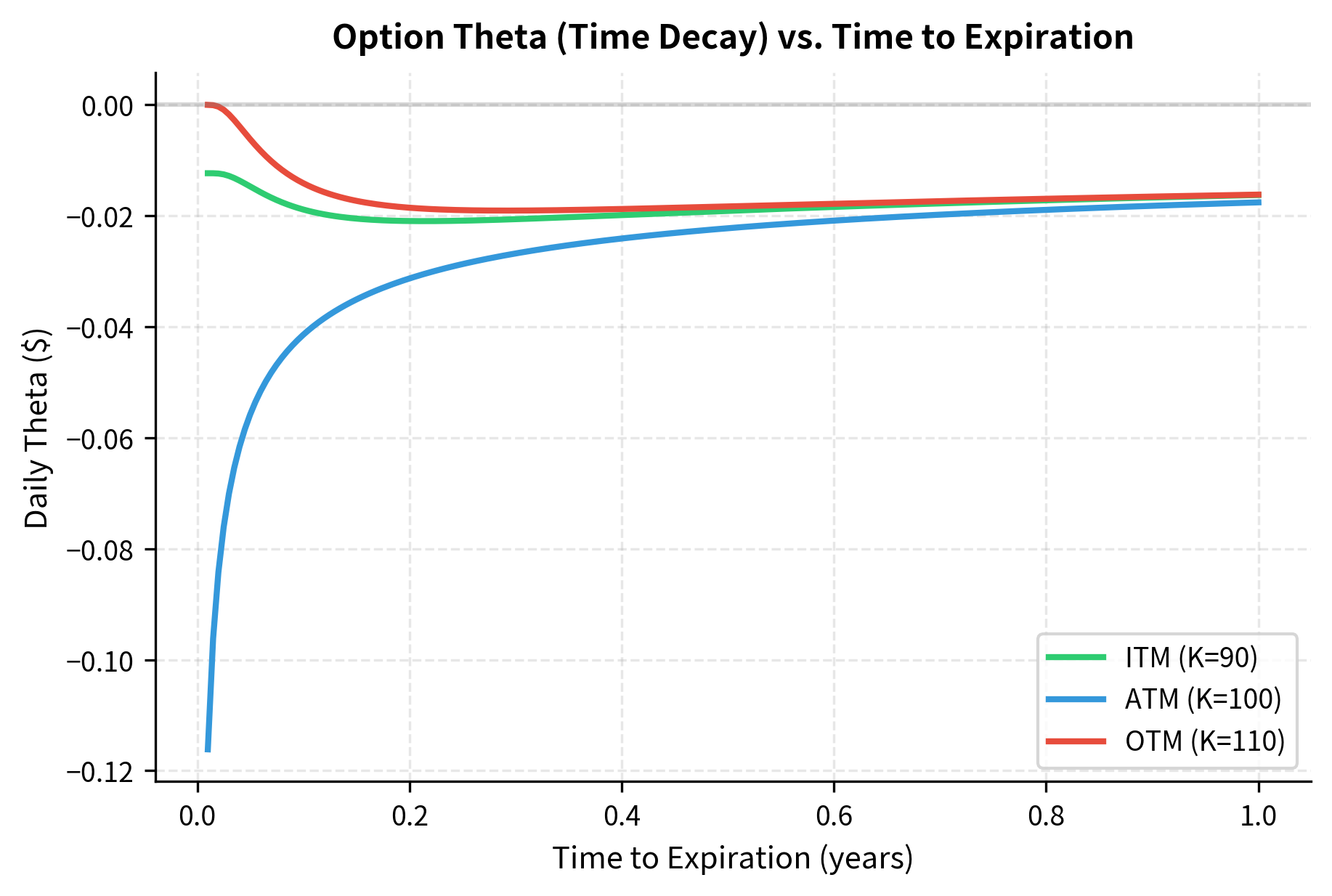
The theta chart shows the characteristic hockey stick shape for at-the-money options: time decay accelerates dramatically in the final weeks before expiration. This pattern has important implications for option trading strategies. You often prefer short-dated options because you collect theta more rapidly; the premium you receive decays quickly in your favor. Conversely, you face intensifying time decay pressure as expiration approaches, which is why you often roll your long option positions to later expirations before the theta erosion becomes severe.
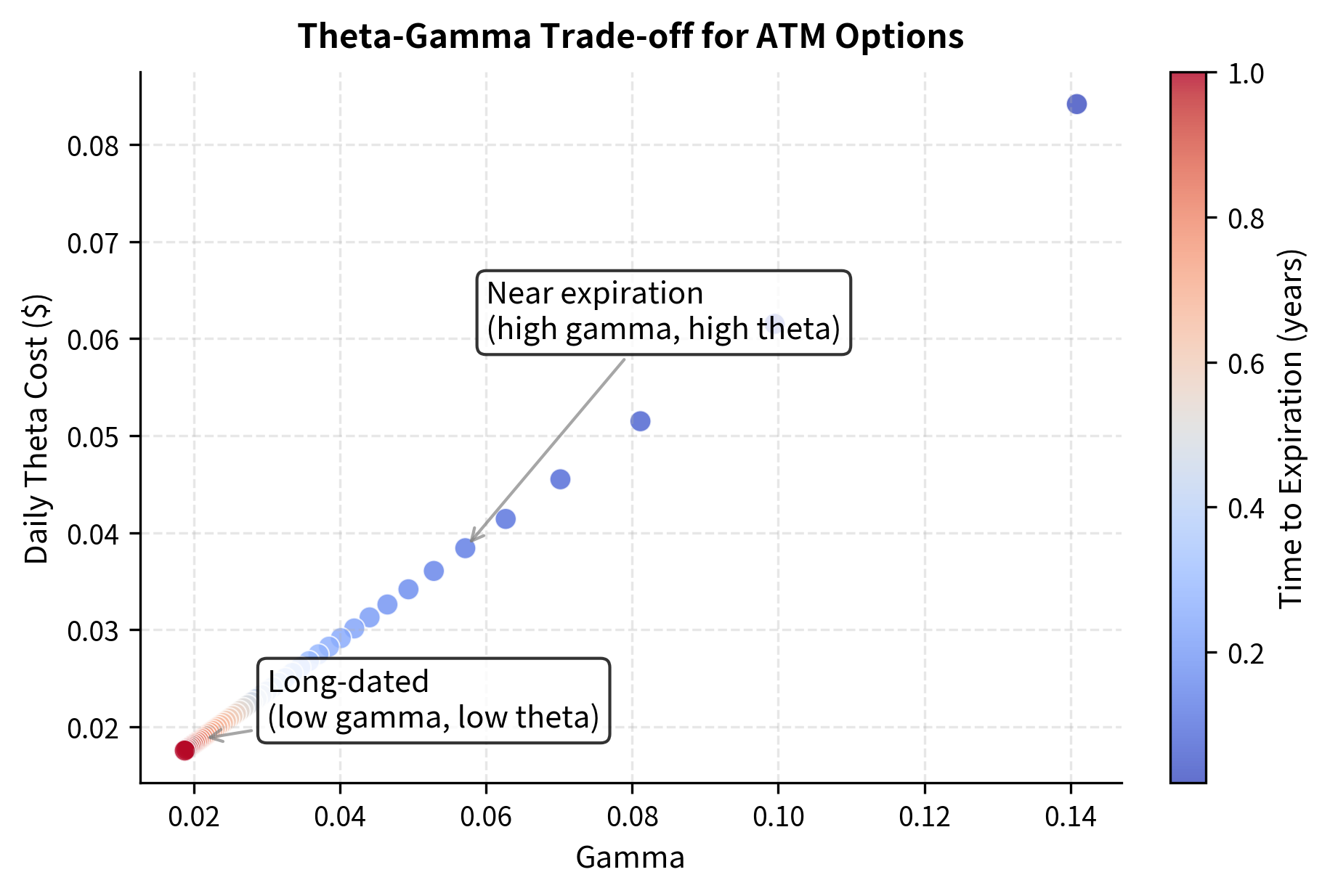
The theta-gamma trade-off visualization demonstrates a fundamental principle of options: you cannot have high gamma (benefiting from price moves) without paying for it through theta (time decay). Near-expiration ATM options occupy the upper-right region with both high gamma and high theta cost. Longer-dated options have lower values of both. This relationship is not a coincidence but follows directly from the Black-Scholes PDE, which enforces that the benefits of convexity must be paid for through time decay in an arbitrage-free market.
Vega: Sensitivity to Volatility
Vega ( or sometimes ) measures the sensitivity of an option's price to changes in implied volatility. While delta captures exposure to price movements that are directly observable in the market, vega captures exposure to volatility, which is the market's expectation of future price variability. This distinction is crucial because volatility is not directly observable; it must be estimated or implied from option prices themselves.
Mathematically, vega is defined as:
where:
- : option vega
- : option value
- : implied volatility
Despite being called a "Greek," vega is not actually a Greek letter; it's a star name. Nevertheless, it has become standard terminology in options markets, and no serious discussion of option risk can proceed without it.
Vega for European Options
Deriving vega requires differentiating the Black-Scholes formula with respect to volatility . Like theta, volatility appears in multiple places in the formula, including in both and as well as in the scaling of the distribution. After working through the calculus, a remarkably clean result emerges.
For both European calls and puts:
where:
- : option vega
- : underlying price
- : strike price
- : risk-free interest rate
- : volatility
- : time to expiration
- : standard normal PDF
- : standardized moneyness factor
Like gamma, vega is identical for calls and puts with the same parameters, which follows from put-call parity (the right side of the parity relationship doesn't depend on volatility). This symmetry makes intuitive sense: both calls and puts benefit equally from increased uncertainty about future prices, because both options benefit from large moves in their favorable direction.
Understanding Vega
Vega captures exposure to volatility, which is arguably the most important risk factor in options trading. While stock prices are observable in real time, volatility must be estimated or implied from option prices. This inherent uncertainty about the correct volatility makes volatility risk central to options management. We often say that when you trade options, you are really trading volatility, not direction.
The key properties of vega include:
-
Always positive for long options: Higher volatility increases the value of both calls and puts because it increases the probability of large moves, which benefit option holders. Whether you hold a call hoping for a big move up or a put hoping for a big move down, more volatility increases your chances of success.
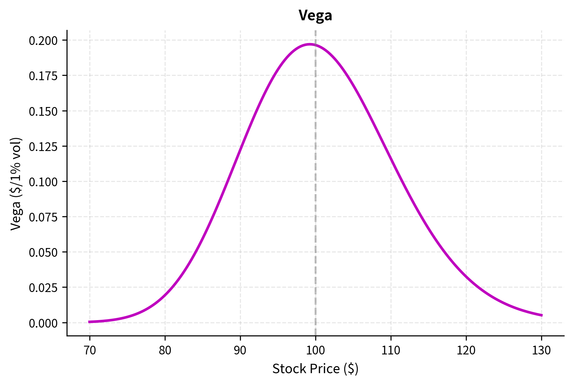
-
Maximum at-the-money: ATM options have the highest vega because their value is most sensitive to the probability of ending up in the money, which volatility directly affects. An at-the-money option is balanced between having value and being worthless, so changes in the expected distribution of future prices matter most.
-
Increases with time: Unlike gamma (which increases near expiration), vega increases with time to expiration because there's more time for volatility to have an effect. Over a longer horizon, volatility has more opportunity to compound and produce large cumulative price movements.
Our vega implementation calculates the sensitivity to volatility. Note that while input volatility is typically a decimal (e.g., 0.20), we often speak of vega per 1% change in vol, which requires dividing the result by 100:
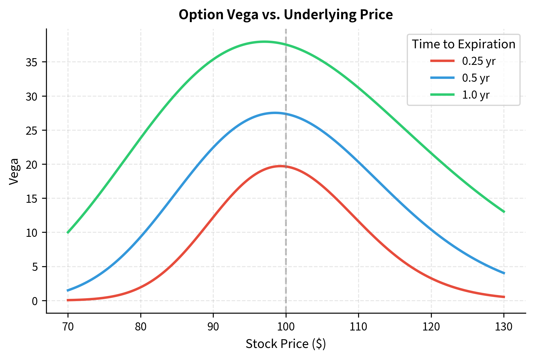
The relationship between vega and time is critical for volatility trading strategies. If you believe volatility will increase, you want long vega exposure, and longer-dated options provide more vega per dollar invested. However, this also means longer-dated options carry more volatility risk if your view is wrong. The choice between short-dated and long-dated options for a volatility trade involves balancing the magnitude of vega exposure against the cost of theta and the risk of being wrong about the timing of volatility changes.
Rho: Interest Rate Sensitivity
Rho () measures the sensitivity of an option's price to changes in the risk-free interest rate. While less prominent than the other Greeks, rho becomes important for long-dated options and in environments where interest rates are changing significantly.
Mathematically, rho is defined as:
where:
- : option rho
- : option value
- : risk-free interest rate
Rho reflects how the risk-free rate affects option value by discounting future cash flows. For a call option, you will pay the strike price at expiration if the option is exercised. A higher interest rate reduces the present value of this future payment, making the call more valuable today. For a put option, you receive the strike price upon exercise, so a higher interest rate reduces the present value of this future receipt, making the put less valuable.
Rho for European Options
The derivation of rho involves differentiating the Black-Scholes formula with respect to the interest rate . The rate appears both in the discount factor and in the and terms. After working through the mathematics, we obtain clean expressions.
For a European call option:
where:
- : rho of a European call
- : underlying price
- : strike price
- : risk-free interest rate
- : volatility
- : time to expiration
- : probability factor
- : probability factor adjusting for time and volatility
- : probability factor adjusting for volatility drag
The formula shows that rho is proportional to both the strike price and the time to expiration . This makes intuitive sense: the effect of discounting is larger for higher strike prices and for longer periods. The factor , which represents the risk-neutral probability of exercise, scales the effect by how likely it is that the interest rate change will actually matter.
For a European put option:
where:
- : rho of a put option
- : underlying price
- : strike price
- : risk-free interest rate
- : volatility
- : time to expiration
- : negative probability factor
- : probability factor adjusting for time and volatility
- : probability factor adjusting for volatility drag
The Lesser Greek
Among the standard five Greeks, rho typically receives the least attention. This is because:
-
Interest rates are relatively stable: Day-to-day interest rate changes are usually small compared to moves in stock prices or volatility. Stock prices can easily move several percent in a day, while interest rate changes of even a few basis points are noteworthy.
-
Effect is often small: For typical options with moderate maturities, rho is small relative to other Greeks. A three-month option on a $100 stock might have a vega of 20 (meaning a 1% vol change moves the price by $0.20) but a rho of only 5 (meaning a 1% rate change moves the price by $0.05).
-
Magnitude increases with time: Rho is proportional to time to expiration, so it becomes relevant for LEAPS, long-term equity anticipation securities, and long-dated options where the discounting effect operates over a longer horizon.
We define rho for both calls and puts below. The formula captures the sensitivity of the present value of the strike price to interest rates:
The intuition for rho is straightforward: a higher interest rate reduces the present value of the strike price (which you'll pay in the future for a call or receive for a put). This reduction benefits call holders and hurts put holders, hence the positive rho for calls and negative for puts.
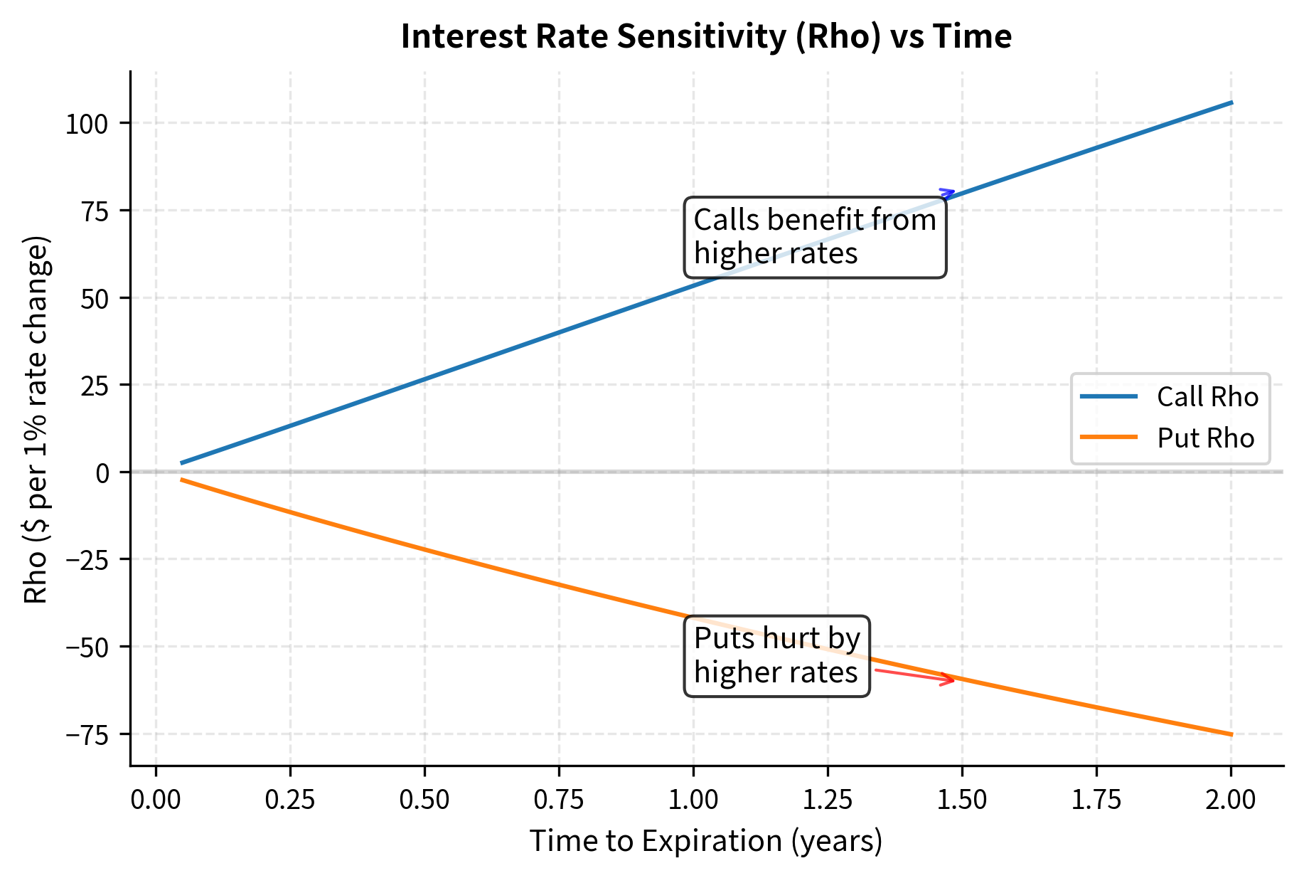
The rho visualization confirms the key insight that interest rate sensitivity grows with time to expiration. For short-dated options (under three months), rho is relatively small and often ignored. However, for LEAPS with two-year expirations, a 1% change in interest rates can move the option price by several dollars. This becomes particularly relevant during periods of monetary policy transitions when rates change significantly.
Greeks as a Taylor Expansion
The Greeks provide a powerful way to approximate how an option's value will change when multiple market parameters shift simultaneously. This approximation is based on a Taylor series expansion, the same mathematical tool we developed in Part I for approximating functions near a point. The Taylor expansion allows us to decompose complex changes in option value into contributions from each risk factor.
First-Order Approximation
For small changes in the underlying inputs, we can write:
where:
- : change in option price
- : option delta
- : change in stock price
- : passage of time
- : change in implied volatility
- : change in interest rate
- : option theta
- : option vega
- : option rho
This first-order approximation is linear in each parameter and forms the basis of daily P&L attribution in trading operations. Each Greek acts as a coefficient that translates a change in its corresponding market variable into a contribution to profit or loss. By examining these contributions separately, we can understand why our positions made or lost money and can identify which risk factors drove the result.
Second-Order Approximation
To improve accuracy, especially for larger moves, we include the second-order term:
where:
- : change in option price
- : option delta
- : change in stock price
- : option gamma
- : squared change in stock price (convexity term)
- : option theta
- : passage of time
- : option vega
- : change in implied volatility
- : option rho
- : change in interest rate
The gamma term is particularly important because options are non-linear instruments. For large stock moves, the term can dominate the linear term. Consider a stock that moves $10; the delta contribution is , but the gamma contribution is . Even if gamma is much smaller than delta in absolute terms, the square of the price move amplifies its effect significantly.
P&L Attribution Example
Let's see how this works in practice. First, we define a pricing function to establish the baseline value. Then, we simulate a market move involving simultaneous changes in price, time, and volatility to compare the first-order (Delta, Vega, Theta) and second-order (Gamma) approximations against the actual P&L:
The second-order approximation captures the convexity effect and provides a much more accurate estimate. This is why gamma is essential for risk management; relying only on delta can significantly underestimate P&L for larger moves. In this example, the gamma term accounts for the difference between the first-order and second-order estimates, demonstrating the practical importance of understanding option curvature.
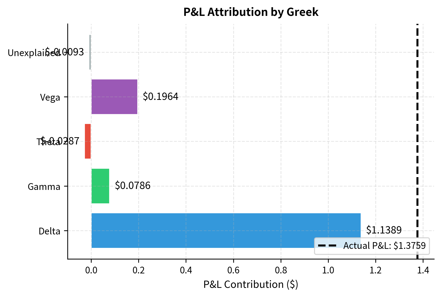
The P&L attribution chart makes clear how each risk factor contributed to the total profit. In this scenario, the stock price increase generated positive delta P&L, while the volatility increase added vega P&L. The theta contribution was slightly negative (time decay), and the gamma contribution captured the non-linearity. The small unexplained residual represents higher-order effects not captured by the second-order Taylor expansion.
Delta Hedging and Delta-Neutral Portfolios
Delta hedging is the practice of trading the underlying asset to offset the delta of an option position, creating a portfolio that is (to first order) immune to small price movements. This technique is fundamental to options market making and forms the basis of more sophisticated hedging strategies.
Constructing a Delta-Neutral Position
If you own a call option with , your portfolio gains $0.60 for every $1 increase in the stock. To neutralize this exposure, you short 0.6 shares. The combined position has:
where:
- : net delta of the position
- : delta of the option
- : delta of the stock (always 1)
A delta-neutral portfolio does not profit or lose from small movements in the underlying price. This allows you to isolate other sources of profit or risk, such as time decay or volatility changes. You typically maintain delta-neutral books so you can focus on earning the bid-ask spread without taking directional risk.
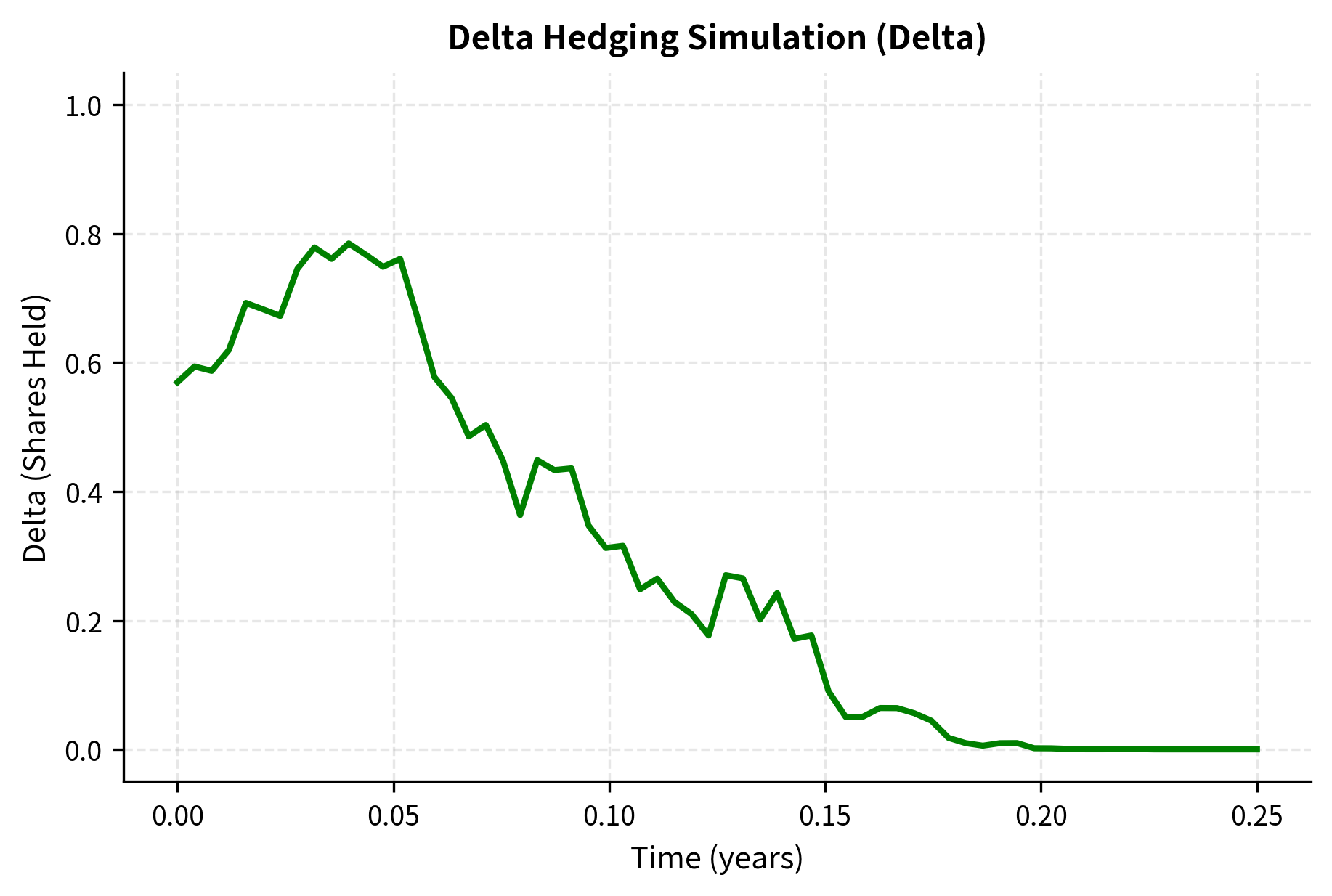
Dynamic Hedging
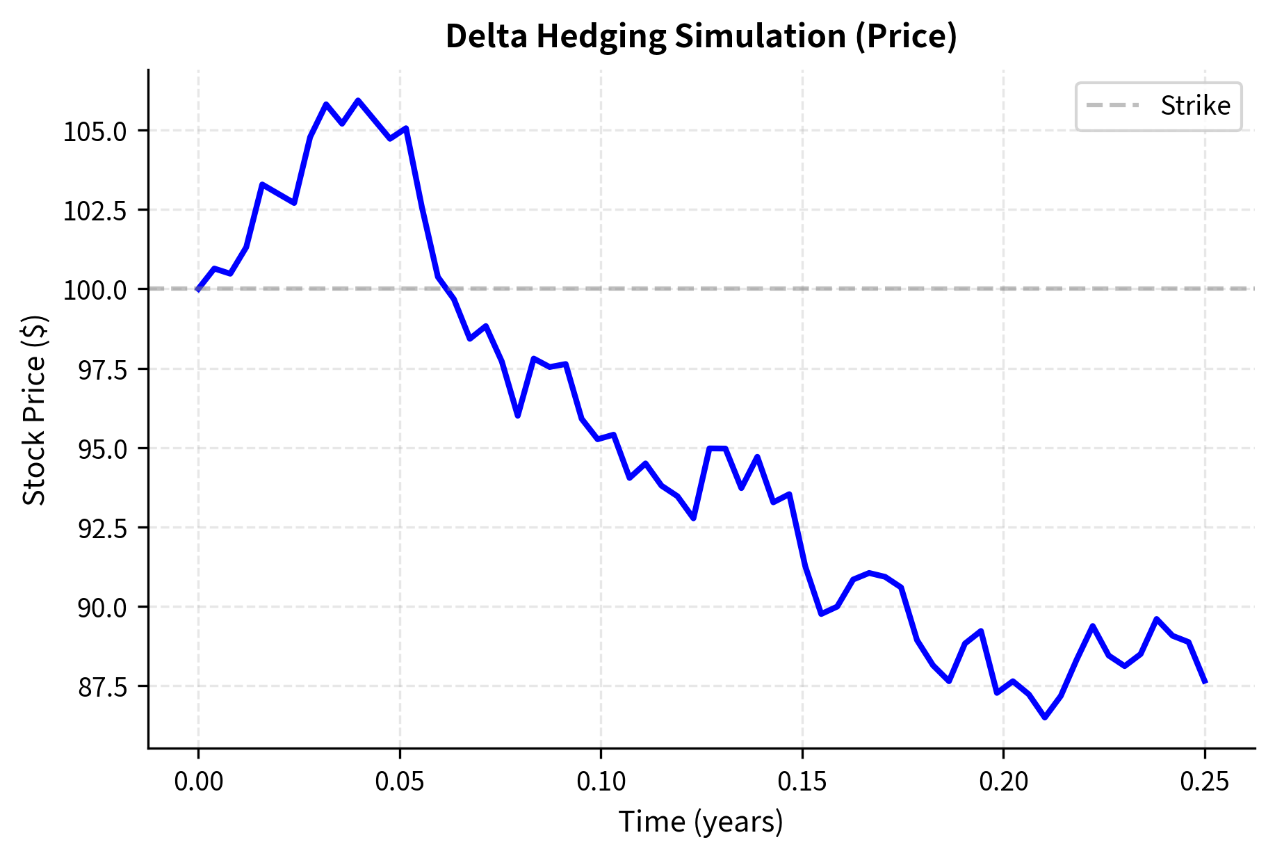
The hedge is only valid at a point in time. As the stock price moves, delta changes (that's gamma), so you must continuously rebalance. In practice, you rehedge at discrete intervals, perhaps hourly or daily, or when delta drifts beyond a threshold. The frequency of rebalancing involves a trade-off: more frequent hedging keeps the portfolio closer to delta-neutral but incurs more transaction costs.
The following simulation demonstrates dynamic hedging. We generate a geometric Brownian motion price path and rebalance the hedge at each time step, tracking the cash flow and shares held to verify if the portfolio value tracks the option price:
Hedging Costs and Gamma
Delta hedging is not free. Each rebalancing trade incurs transaction costs (bid-ask spread, commissions). Moreover, the hedging process itself has an expected cost related to gamma and realized volatility.
When you're short gamma (short options), you systematically buy high and sell low: you buy more shares after the stock rises and sell shares after the stock falls. This "buying high, selling low" pattern loses money on average when volatility is positive, which is the theta you earn for being short options. You earn theta precisely because you must engage in this unfavorable trading pattern to maintain your hedges.
Conversely, when you're long gamma, you sell high and buy low during rebalancing, capturing the realized volatility. This is the core mechanism behind volatility arbitrage strategies. If you buy an option at an implied volatility of 20% and the stock actually realizes 25% volatility, your gains from delta hedging will exceed your losses from theta, generating a profit.
Gamma and Vega Risk Management
While delta hedging handles directional risk, managing a professional option portfolio requires controlling gamma and vega exposures as well. These higher-order risks can dominate P&L during volatile market conditions and require specific techniques to manage.
Gamma Hedging
You cannot hedge gamma using the underlying asset alone because stock has zero gamma. The delta of a stock is always 1, regardless of the stock price, so its gamma is zero. To adjust gamma, you must trade other options.
Suppose your portfolio has and you want to make it gamma-neutral. You can add a position in another option with known gamma . The number of options to trade is:
where:
- : number of hedging options to trade
- : current portfolio gamma
- : gamma of the hedging instrument
After adding this position, you'll need to readjust delta because the new options have delta too. This sequential hedging process, first neutralizing gamma with options and then neutralizing delta with stock, is standard practice in professional trading.
Vega Hedging
Similarly, vega can only be hedged with other options. A portfolio of options on the same underlying will typically have correlated vega exposures; if implied volatility rises, all options tend to gain value.
You often distinguish between:
- Parallel vega risk: Uniform shifts in volatility across all strikes and expirations
- Skew risk: Changes in the volatility smile (the pattern of implied volatility across strikes)
- Term structure risk: Changes in the relationship between short-dated and long-dated implied volatilities
We'll explore these concepts in depth in the next chapter on implied volatility and the volatility smile.
Building a Greek-Neutral Portfolio
Let's work through an example of constructing a portfolio that is simultaneously delta-neutral and gamma-neutral. We first calculate the Greeks for our existing position and a hedging instrument. Then, we solve a system of linear equations: first finding the quantity of the hedging option to neutralize gamma, and then using stock to neutralize the remaining delta:
The hedged portfolio is now immune (to second order) to moves in the underlying. However, it still has theta and vega exposure. Managing all Greeks simultaneously requires trading multiple options with different characteristics. In practice, we often accept some residual Greek exposure rather than attempting perfect neutrality, which would be prohibitively expensive in transaction costs.
Higher-Order Greeks
Beyond the standard five Greeks, several higher-order sensitivities become important for sophisticated risk management. These cross-partial derivatives capture how the primary Greeks change when other market variables move, providing a more complete picture of option risk dynamics.
Vanna: Sensitivity of Delta to Volatility
Vanna measures how delta changes when volatility changes:
where:
- Vanna: sensitivity of delta to volatility
- : delta
- : volatility
- : vega
- : spot price
This cross-partial derivative matters when both spot and volatility move together, as they often do in equity markets (where volatility tends to spike when prices fall). The equality between and follows from the symmetry of mixed partial derivatives, a consequence of the smoothness of the Black-Scholes pricing function.
For European options under Black-Scholes:
where:
- : sensitivity of delta to volatility
- : standardized moneyness terms
- : standard normal PDF
- : vega
- : spot price
- : volatility
- : time to expiration
Volga (Vomma): Sensitivity of Vega to Volatility
Volga or vomma measures the convexity of option value with respect to volatility:
where:
- Volga: sensitivity of vega to volatility
- : option value
- : vega
- : volatility
This becomes important when volatility itself is volatile. A portfolio with high volga benefits when realized volatility of implied volatility is high. In markets where implied volatility swings dramatically, volga exposure can dominate P&L.
Charm: Sensitivity of Delta to Time
Charm measures how delta changes as time passes:
where:
- Charm: sensitivity of delta to time
- : delta
- : time
- : theta
- : spot price
This is important for understanding how your hedge will need to change even if the spot price remains constant. A position that is delta-neutral today may drift away from neutrality simply due to the passage of time, requiring rebalancing.
Speed: Sensitivity of Gamma to Price
Speed is the third derivative of option price with respect to spot:
where:
- Speed: sensitivity of gamma to price
- : option value
- : gamma
- : spot price
Speed matters when gamma itself is highly sensitive to price movements. For large portfolios of options with different strikes, understanding speed helps us anticipate how our gamma exposure will change during market moves.
We can calculate these higher-order Greeks using the formulas derived from the Black-Scholes partial derivatives. These values help quantify the stability of the primary Greeks:
The calculated values provide deeper insight: vanna is negative, meaning delta decreases as volatility rises. Volga is positive, indicating vega increases with volatility. Charm is negative, showing delta decay over time. While these higher-order Greeks may seem esoteric, they become critical when managing large option portfolios or when market conditions are extreme. In the 2008 and 2020 crashes, ignoring higher-order Greeks often led to unexpected losses as simple models failed to capture complex risk interactions.
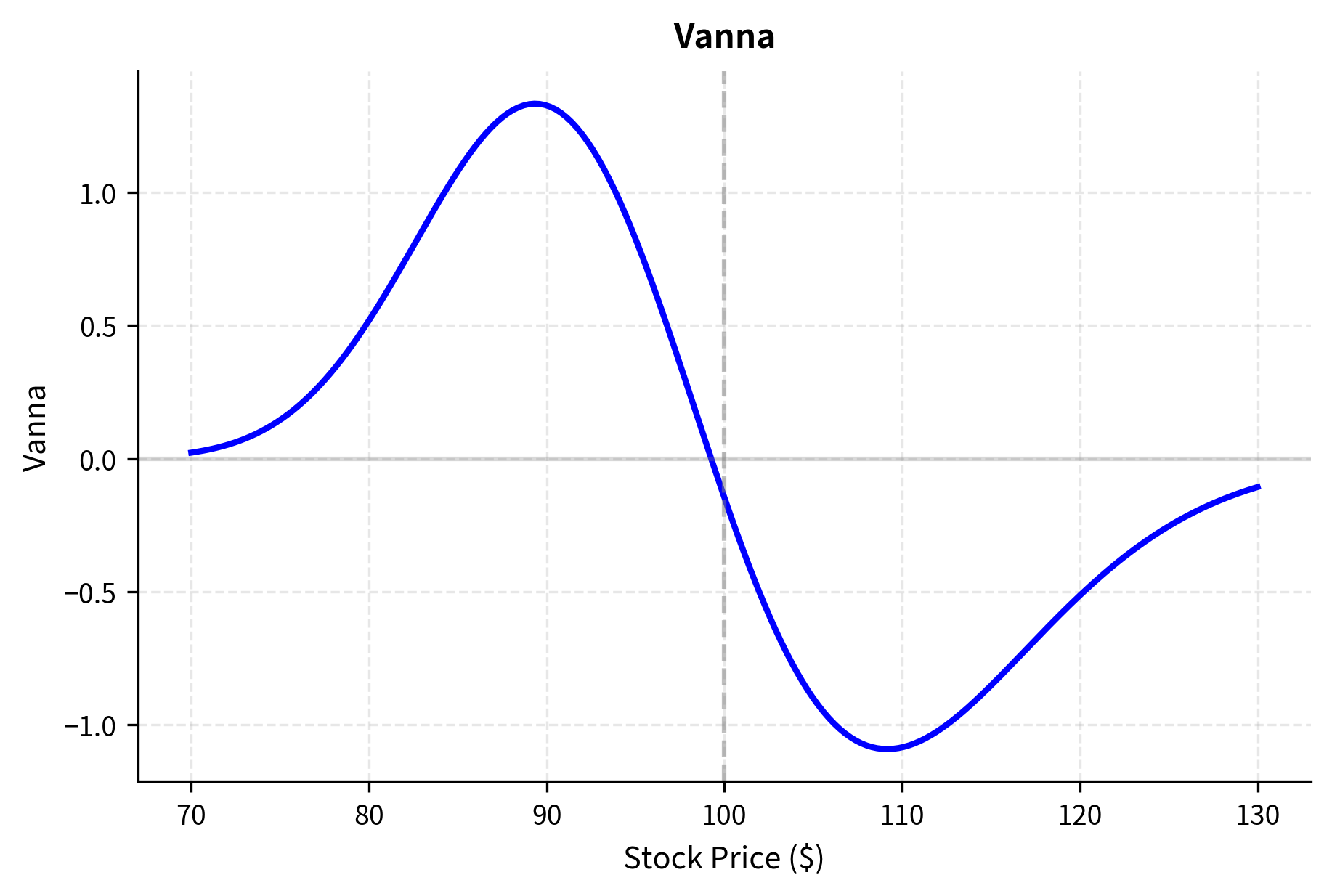
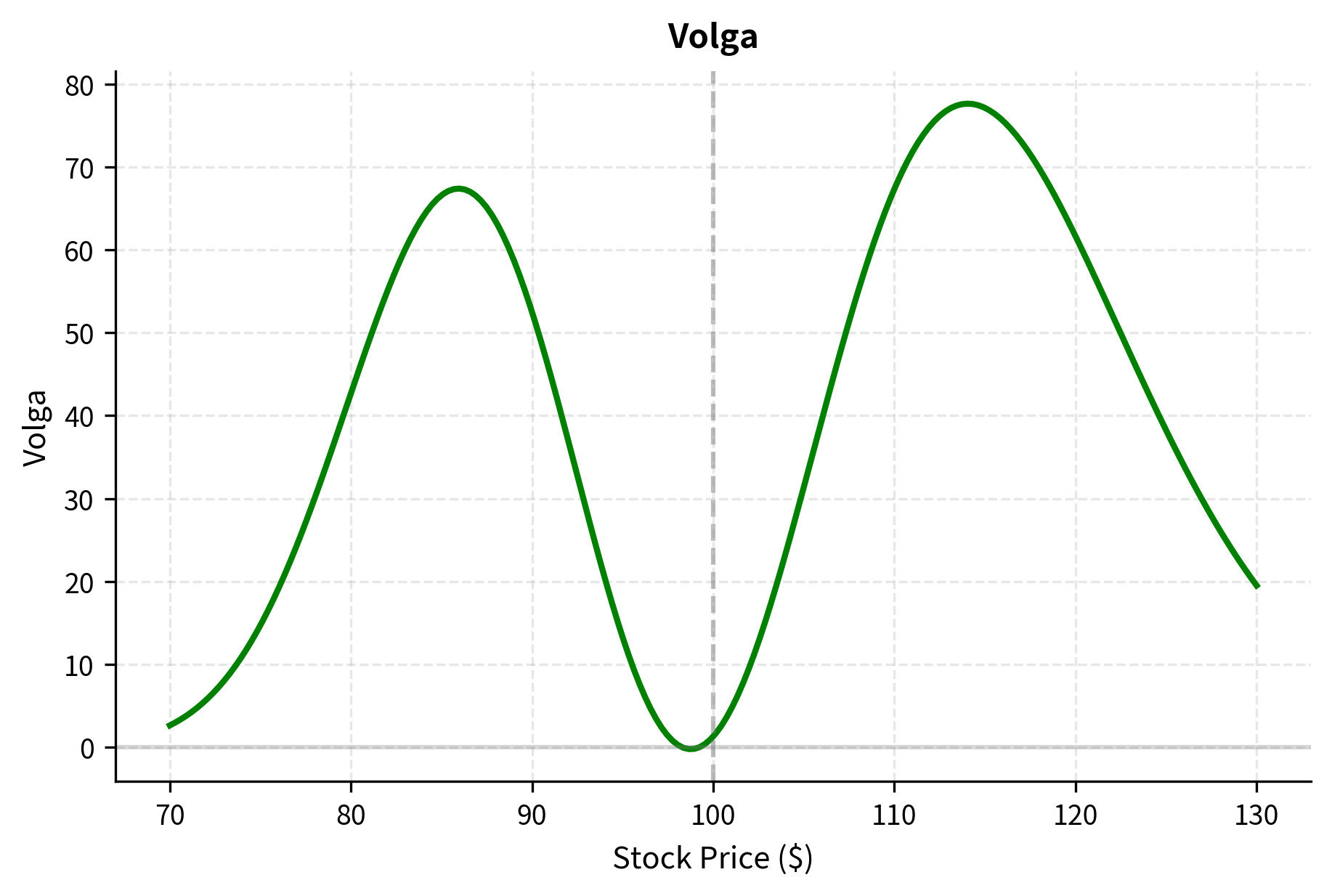
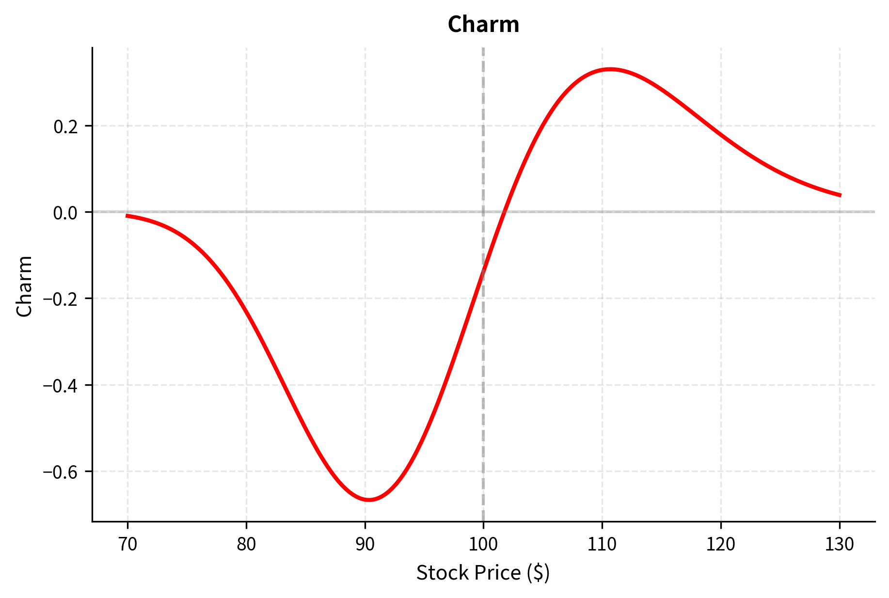
The higher-order Greeks profiles reveal important asymmetries. Vanna is negative for ITM options and positive for OTM options, meaning volatility changes affect delta differently depending on moneyness. Volga is positive everywhere but peaks slightly away from ATM, indicating that volatility convexity is greatest for slightly OTM options. Charm shows that delta drifts toward extreme values (0 or 1) as time passes, with the fastest drift occurring near the strike.
Comprehensive Greeks Calculator
Let's bring everything together in a complete implementation that calculates all Greeks and visualizes the risk profile of an option position. We encapsulate the logic in a class to manage the parameters and calculations cleanly, providing methods for each Greek and a summary report:
The table demonstrates the fundamental parity relationships. Gamma and vega are identical for calls and puts with the same parameters, illustrating that curvature and volatility risks are independent of direction. Delta values diverge, reflecting the opposing directional views, while theta remains negative for both long positions.

The profile shows how each Greek behaves as the stock price changes. Delta rises from 0 to 1 as the option goes from OTM to ITM. Gamma peaks where delta changes fastest (ATM). Theta is most negative ATM where time value is highest. Vega also peaks ATM, showing that volatility sensitivity is concentrated near the strike.
Option Portfolio Risk Reports
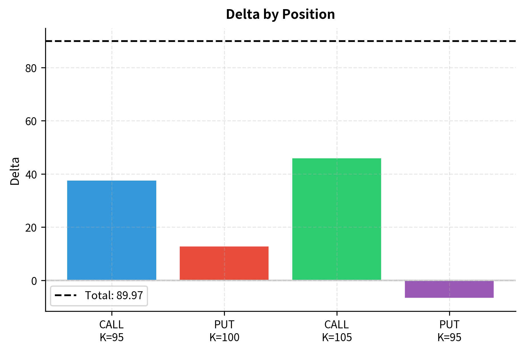
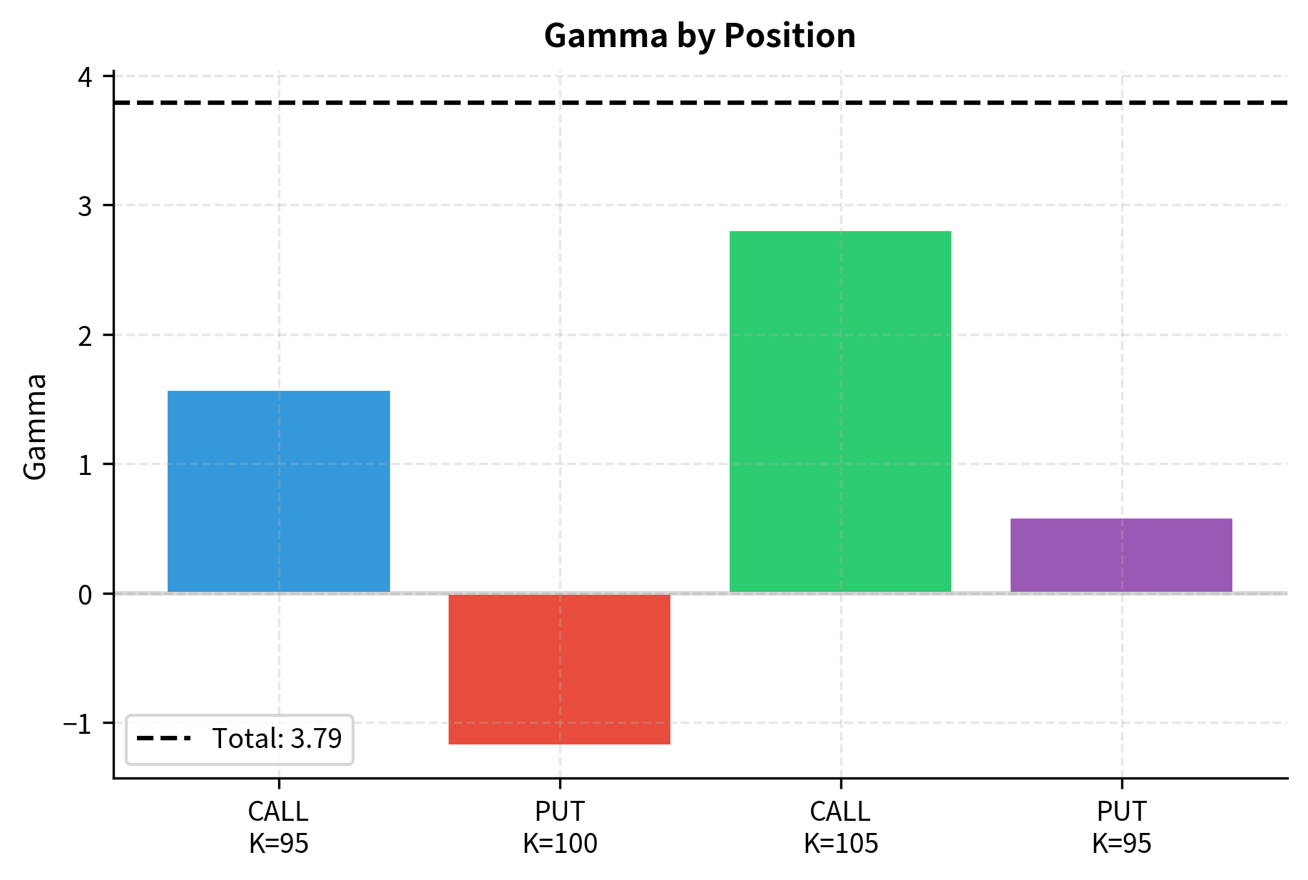
In practice, we work with entire portfolios of options rather than individual positions. A typical risk report aggregates Greeks across all positions. In the code below, we define a portfolio of mixed positions, calculate the Greeks for each, and sum them to determine the net portfolio exposure:
This type of report allows you to quickly understand your exposures and decide whether to hedge. The portfolio above is long delta, meaning it benefits from rising stock prices (gaining approximately the delta amount for a $1 increase. It is also long gamma and vega, meaning the position value increases with both large market moves and rising volatility. However, these benefits come at a cost: the negative theta indicates the portfolio loses value daily due to time decay.
#| label: fig-portfolio-theta #| echo: false #| output: true #| fig-cap: "Portfolio theta contribution by position. Long options incur negative theta (time decay cost), while short options earn positive theta. The net theta represents the daily carry cost of the portfolio." #| fig-alt: "Bar chart showing theta contributions." #| fig-file-name: portfolio-theta.png
plt.rcParams.update({ "figure.figsize": (6.0, 4.0), "figure.dpi": 300, "figure.constrained_layout.use": True, "font.family": "sans-serif", "font.sans-serif": ["Noto Sans CJK SC", "Apple SD Gothic Neo", "DejaVu Sans", "Arial"], "font.size": 10, "axes.titlesize": 11,
Quiz
Ready to test your understanding? Take this quick quiz to reinforce what you've learned about option Greeks and risk management.

Comments