Term Structure of Interest Rates: Yield Curve Construction

Michael Brenndoerfer

Master yield curve construction through zero rates, forward rates, and bootstrapping. Learn to interpret curve shapes and build production-quality curves.

Track your reading progress

Sign in to mark chapters as read and track your learning journey

Sign in →

Reading Level

Choose your expertise level to adjust how many terms are explained. Beginners see more tooltips, experts see fewer to maintain reading flow. Hover over underlined terms for instant definitions.

Term Structure of Interest RatesLink Copied

The term structure of interest rates describes how interest rates vary across different maturities at a single point in time. When you deposit money at a bank, the rate you receive for a 1-year certificate of deposit typically differs from the rate for a 5-year CD. This observation has direct implications for pricing bonds, valuing derivatives, and understanding market expectations about future economic conditions.

The graphical representation of this relationship is called the yield curve. Every morning, traders, portfolio managers, and central bankers examine the yield curve to gauge market sentiment, identify relative value opportunities, and make policy decisions. The shape of the curve, whether upward sloping, flat, or inverted, encodes collective market expectations about inflation, economic growth, and monetary policy.

Understanding the term structure is essential for fixed-income valuation. Every bond price, interest rate swap, and fixed-income derivative depends on discount rates that vary with maturity. A single "interest rate" is a fiction. In practice, you need an entire curve of rates. This chapter develops the tools to construct, interpret, and apply this curve.

Fundamental Rate ConceptsLink Copied

Before constructing yield curves, you need to understand three related but distinct types of interest rates: zero rates, spot rates, and forward rates. These concepts form the vocabulary of fixed-income analysis. While they might initially seem like different names for similar ideas, each captures a subtly different aspect of how money grows over time. Mastering these distinctions is essential because they appear throughout fixed-income valuation, from the simplest bond pricing to the most complex derivative structures.

These rate concepts are different lenses for viewing the same underlying economic reality, the time value of money. Zero rates tell you what return you earn by locking up money today until some future date. Forward rates reveal what the market implies about borrowing costs in future periods. Discount factors translate future cash flows into present values. Together, they provide a complete toolkit for analyzing any stream of payments across time.

Zero-Coupon RatesLink Copied

Zero-Coupon Rate

A zero-coupon rate (or zero rate) is the interest rate earned on an investment that starts today and makes a single payment at maturity with no intermediate cash flows. It represents the pure time value of money for a specific horizon.

Zero-coupon rates are the building blocks of fixed-income valuation. Their power lies in their simplicity. Because there are no intermediate payments, a zero rate captures the pure relationship between present and future value for a specific time horizon. This purity makes zero rates the natural starting point for understanding how money grows over time.

Consider a zero-coupon bond that pays $100 in$ T $years and trades today at price$ P $. The fundamental question is: what annualized rate of return does this investment offer? The zero rate$ z(T)$ satisfies:

P = 100 \cdot e^{-z(T) \cdot T}

where:

$P$ : current market price of the zero-coupon bond
$T$ : time to maturity in years
$z(T)$ : continuously compounded zero rate for maturity $T$
$e^{-z(T) \cdot T}$ : the discount factor, representing how much $1 received at time $T$ is worth today

This equation shows that the price you pay today equals the future payment discounted back at the appropriate rate. The exponential form arises from continuous compounding, where interest accrues at every instant rather than at discrete intervals. Using continuous compounding simplifies many formulas and is standard in quantitative finance, even though actual market quotes often use different conventions.

Solving for the zero rate reveals how to extract the implied rate from observable prices:

\begin{aligned} P &= 100 \cdot e^{-z(T) \cdot T} && \text{(starting equation)} \\ \frac{P}{100} &= e^{-z(T) \cdot T} && \text{(divide by face value)} \\ \ln\left(\frac{P}{100}\right) &= -z(T) \cdot T && \text{(take natural log)} \\ z(T) &= -\frac{1}{T} \ln\left(\frac{P}{100}\right) && \text{(solve for } z(T) \text{)} \end{aligned}

The zero rate tells you the annualized return for locking up money from today until maturity $T$ . Because there are no intermediate payments, there's no reinvestment risk, and you know exactly what return you'll earn. This certainty is precisely what makes zero rates so valuable as building blocks: they provide unambiguous rates for specific maturities without the complications introduced by coupon payments that must be reinvested at unknown future rates.

Spot Rates and Their Relationship to Zero RatesLink Copied

The terms "spot rate" and "zero rate" are often used interchangeably, though technically they have subtle distinctions. A spot rate refers to the current market rate for immediate delivery of a financial instrument. In the context of interest rates, the spot rate for maturity $T$ is the rate at which you can borrow or lend today for delivery (settlement) right now, with repayment at time $T$ .

For practical purposes in yield curve analysis, spot rates and zero rates are the same thing: they both represent the current rate for a single-payment instrument maturing at time $T$ . The term "zero rate" emphasizes the zero-coupon nature of the instrument, while "spot rate" emphasizes that it's the current market rate (as opposed to a forward rate). When you encounter these terms in practice, context usually makes the intended meaning clear, but understanding the subtle distinction helps you navigate financial literature with confidence.

Discount FactorsLink Copied

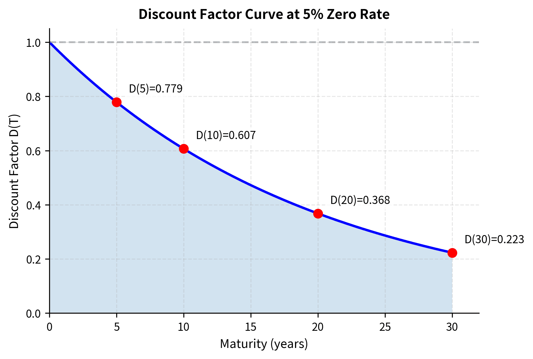
While zero rates express the time value of money as an interest rate, discount factors express the same concept as a multiplier. The discount factor $D(T)$ represents the present value today of receiving $1 at time $T$ :

D(T) = e^{-z(T) \cdot T}

where:

$D(T)$ : discount factor for maturity $T$ (a number between 0 and 1)
$z(T)$ : continuously compounded zero rate for maturity $T$
$T$ : time to maturity in years

Intuitively, the discount factor answers a simple question: how much would I pay today for a guaranteed $1 in $T$ years? Higher interest rates or longer maturities produce smaller discount factors, reflecting the greater opportunity cost of waiting. A discount factor of 0.95 for one year means that $1 next year is worth $0.95 today. You would need to invest $0.95 now at the prevailing rate to have exactly $1 in one year.

Discount factors provide a direct way to value any cash flow stream. For a bond paying cash flows $C_1, C_2, \ldots, C_n$ at times $t_1, t_2, \ldots, t_n$ , the price is simply the sum of each cash flow multiplied by its corresponding discount factor:

P = \sum_{i=1}^{n} C_i \cdot D(t_i)

where:

$P$ : present value (price) of the bond
$C_i$ : cash flow received at time $t_i$
$D(t_i)$ : discount factor for maturity $t_i$
$n$ : total number of cash flows

This formula shows why zero rates matter: they determine the discount factors that price all fixed-income securities. Whether you're valuing a simple Treasury bond, a complex mortgage-backed security, or an exotic interest rate derivative, the fundamental operation is the same: multiply each future cash flow by the appropriate discount factor and sum the results.

Out[2]:

Visualization

Discount factors D(T) for maturities from 0 to 30 years at a constant 5% zero rate. The exponential decay curve demonstrates how the present value of $1 received in the future decreases monotonically with time, dropping from $1.00 at maturity 0 to approximately $0.22 at 30 years. The rate of decay accelerates for longer maturities, reflecting the compounding effect of the time value of money.

Forward RatesLink Copied

Forward Rate

A forward rate is the interest rate implied by current spot rates for a loan that begins at a future date $T_1$ and matures at a later date $T_2$ . It represents the rate that can be locked in today for future borrowing or lending.

Forward rates extend our understanding of the term structure by answering a natural question. If we know today's rates for various maturities, what does the market imply about rates in the future? This is not merely an academic exercise. Forward rates have practical applications. Financial institutions use forward rate agreements (FRAs) to lock in borrowing costs for future periods, and the forward rates embedded in the yield curve are the fair prices for these contracts.

Suppose you know the zero rates for 1 year and 2 years. What rate can you lock in today for borrowing during the second year? This is the 1-year forward rate starting in 1 year, denoted $f(1,2)$ .

The logic relies on a no-arbitrage argument, which is one of the most powerful concepts in finance. No-arbitrage reasoning asks a simple question. If two strategies produce the same outcome, they must have the same cost. Otherwise, traders could profit risklessly by buying the cheap strategy and selling the expensive one. Consider two equivalent strategies for investing $1 for two years:

Direct investment: Invest $1 for 2 years at rate$ z(2) $, receiving$ e^{z(2) \cdot 2}$
Sequential investment: Invest $1 for 1 year at rate$ z(1) $, then reinvest the proceeds for another year at the forward rate$ f(1,2) $, receiving$ e^{z(1) \cdot 1} \cdot e^{f(1,2) \cdot 1}$

Both strategies start with $1 today and end with cash in two years. The direct investment locks in a known outcome immediately. The sequential investment achieves the same outcome if the forward rate is correctly priced. You can enter into a forward rate agreement today that guarantees the rate for the second year. For no arbitrage, these must be equal:

e^{z(2) \cdot 2} = e^{z(1) \cdot 1} \cdot e^{f(1,2) \cdot 1}

Solving step by step to extract the forward rate:

\begin{aligned} e^{z(2) \cdot 2} &= e^{z(1) \cdot 1} \cdot e^{f(1,2) \cdot 1} && \text{(no-arbitrage condition)} \\ e^{z(2) \cdot 2} &= e^{z(1) + f(1,2)} && \text{(combine exponents)} \\ z(2) \cdot 2 &= z(1) + f(1,2) && \text{(take natural log of both sides)} \\ f(1,2) &= 2 \cdot z(2) - z(1) && \text{(solve for forward rate)} \end{aligned}

This derivation reveals a fundamental relationship: the forward rate is determined entirely by the two endpoint zero rates. No additional market information is needed. The forward rate is fully implied by the spot curve.

More generally, the forward rate between times $T_1$ and $T_2$ is:

f(T_1, T_2) = \frac{z(T_2) \cdot T_2 - z(T_1) \cdot T_1}{T_2 - T_1}

where:

$f(T_1, T_2)$ : forward rate for the period from $T_1$ to $T_2$
$z(T_1), z(T_2)$ : zero rates for maturities $T_1$ and $T_2$
$T_2 - T_1$ : length of the forward period in years

The numerator represents the difference in accumulated "interest" (rate times time) between the two maturities. Dividing by the length of the forward period converts this to an annualized rate applicable to that specific interval.

This can also be expressed using discount factors:

f(T_1, T_2) = \frac{1}{T_2 - T_1} \ln\left(\frac{D(T_1)}{D(T_2)}\right)

The ratio $D(T_1)/D(T_2)$ represents the growth factor from $T_1$ to $T_2$ : it tells you how much $1 at time $T_1$ grows to by time $T_2$ when invested at the forward rate. Since $D(T_2)$ is always smaller than $D(T_1)$ (money farther in the future is worth less today), this ratio exceeds 1, and its logarithm is positive, yielding a positive forward rate.

Instantaneous Forward RatesLink Copied

The forward rate formula naturally leads to a limiting concept: what happens as the forward period shrinks to zero? As the interval shrinks to zero, we obtain the instantaneous forward rate:

f(t) = \lim_{\Delta t \to 0} f(t, t + \Delta t) = -\frac{d \ln D(t)}{dt}

where:

$f(t)$ : instantaneous forward rate at time $t$
$D(t)$ : discount factor for maturity $t$
$\Delta t$ : an infinitesimally small time interval
$\frac{d \ln D(t)}{dt}$ : the rate of change of the log discount factor with respect to time

The instantaneous forward rate represents the marginal rate of interest at each future instant. Specifically, it is the rate you would earn for an infinitesimally short deposit starting at time $t$ . While no actual financial instrument has zero duration, instantaneous forward rates are mathematically convenient because they allow us to describe the entire term structure with a single function $f(t)$ rather than a collection of discrete rates.

The relationship between zero rates and instantaneous forward rates is remarkably elegant:

z(T) = \frac{1}{T} \int_0^T f(t) \, dt

where:

$z(T)$ : zero rate for maturity $T$
$f(t)$ : instantaneous forward rate at time $t$
$\int_0^T f(t) \, dt$ : accumulates all the instantaneous rates from today to maturity $T$

This relationship shows that the zero rate is simply the average of all instantaneous forward rates from today to maturity. Just as your average speed on a trip is total distance divided by total time, the zero rate is the average of all the "speeds," or instantaneous rates, along the way. This interpretation provides insight into the relationship between spot and forward curves: the spot rate to any maturity represents the cumulative effect of all the marginal rates encountered along the path from today to that maturity.

Numerical Example: Computing Forward RatesLink Copied

Let's work through a concrete example to solidify these concepts. Suppose you observe the following zero rates:

Observed zero rates for forward rate calculation.

Maturity (years)	Zero Rate (%)
1	4.0
2	4.5
3	5.0

What is the forward rate for year 2 (i.e., borrowing from year 1 to year 2)?

We apply the forward rate formula, substituting the known zero rates:

\begin{aligned} f(1,2) &= \frac{z(2) \cdot 2 - z(1) \cdot 1}{2 - 1} && \text{(forward rate formula)} \\ &= \frac{0.045 \times 2 - 0.04 \times 1}{1} && \text{(substitute values)} \\ &= \frac{0.09 - 0.04}{1} && \text{(compute products)} \\ &= 0.05 = 5.0\% && \text{(result)} \end{aligned}

And the forward rate for year 3:

\begin{aligned} f(2,3) &= \frac{z(3) \cdot 3 - z(2) \cdot 2}{3 - 2} && \text{(forward rate formula)} \\ &= \frac{0.05 \times 3 - 0.045 \times 2}{1} && \text{(substitute values)} \\ &= \frac{0.15 - 0.09}{1} && \text{(compute products)} \\ &= 0.06 = 6.0\% && \text{(result)} \end{aligned}

Notice that forward rates can be quite different from spot rates. The 1-year forward rate starting in year 2 is 6%, even though the 3-year zero rate is only 5%. This happens because forward rates must be higher to pull up the average when the curve is upward sloping. If you want your cumulative average to keep rising, each new contribution must exceed the current average. The 6% forward rate for year 3 exceeds the 5% zero rate because it needs to pull the three-year average up from where the two-year average (4.5%) left off.

In[3]:

Code

import numpy as np

# Define zero rates (as decimals)
maturities = np.array([1, 2, 3])
zero_rates = np.array([0.04, 0.045, 0.05])

# Calculate forward rates for each year
forward_rates = []
for i in range(len(maturities)):
    if i == 0:
        # First forward rate equals the first spot rate
        f = zero_rates[0]
    else:
        t1 = maturities[i - 1]
        t2 = maturities[i]
        z1 = zero_rates[i - 1]
        z2 = zero_rates[i]
        f = (z2 * t2 - z1 * t1) / (t2 - t1)
    forward_rates.append(f)

forward_rates = np.array(forward_rates)

# Verify the calculation
print(f"Forward rate for year 2: {forward_rates[1] * 100:.1f}%")
print(f"Forward rate for year 3: {forward_rates[2] * 100:.1f}%")

import numpy as np

# Define zero rates (as decimals)
maturities = np.array([1, 2, 3])
zero_rates = np.array([0.04, 0.045, 0.05])

# Calculate forward rates for each year
forward_rates = []
for i in range(len(maturities)):
    if i == 0:
        # First forward rate equals the first spot rate
        f = zero_rates[0]
    else:
        t1 = maturities[i - 1]
        t2 = maturities[i]
        z1 = zero_rates[i - 1]
        z2 = zero_rates[i]
        f = (z2 * t2 - z1 * t1) / (t2 - t1)
    forward_rates.append(f)

forward_rates = np.array(forward_rates)

# Verify the calculation
print(f"Forward rate for year 2: {forward_rates[1] * 100:.1f}%")
print(f"Forward rate for year 3: {forward_rates[2] * 100:.1f}%")

Out[3]:

Console

Forward rate for year 2: 5.0%
Forward rate for year 3: 6.0%

Out[4]:

Console

Maturity  Zero Rate  Forward Rate
-----------------------------------
  1 yr      4.0%       4.0%
  2 yr      4.5%       5.0%
  3 yr      5.0%       6.0%

The forward rates increase from 4.0% to 5.0% to 6.0%, while zero rates only go from 4.0% to 4.5% to 5.0%. The forward rates increase more steeply than the zero rates. This is a mathematical consequence of how averages work: when the average (zero rate) is rising, the marginal rate (forward rate) must be above the average. This relationship is not merely an artifact of our calculations; it reflects how rates compound over time.

Out[5]:

Visualization

Zero rates and forward rates for 1-year, 2-year, and 3-year maturities from the numerical example. Zero rates increase gradually from 4.0% to 5.0%, while forward rates rise more steeply from 4.0% to 6.0%. The forward curve consistently lies above the zero curve, demonstrating that when the term structure slopes upward, forward rates must exceed the corresponding zero rates because they represent marginal rates that pull up the cumulative average.

Bootstrapping the Zero CurveLink Copied

In practice, zero-coupon bonds with long maturities are rare. Most bonds pay periodic coupons, and the quoted yields reflect the averaging effect of multiple cash flows at different points in time. To extract pure zero rates, we use a technique called bootstrapping.

When a bond pays coupons every six months, its yield-to-maturity is a complex average of the zero rates applicable to each payment date. We cannot simply read off zero rates from coupon bond prices. Instead, we must work backward from prices to rates using a clever sequential procedure.

The Bootstrapping AlgorithmLink Copied

Bootstrapping

Bootstrapping is an iterative procedure to extract zero-coupon rates from the prices of coupon-bearing bonds or other instruments. Starting with short-maturity rates, each successive rate is solved for using previously determined rates to discount intermediate cash flows.

The main idea behind bootstrapping is that we can solve for zero rates one at a time, starting from the shortest maturity and working outward. Each step uses the rates we've already determined to handle intermediate cash flows, leaving only one unknown: the rate for the current maturity.

The algorithm works as follows:

Start with the shortest-maturity instrument, which provides the first zero rate directly
For each successive maturity, use the known zero rates to discount all cash flows except the final one
Solve for the unknown zero rate that makes the present value equal to the market price
Repeat for all maturities

Consider a 2-year annual coupon bond with face value $100, coupon rate$ c $, and price$ P $. If we know the 1-year zero rate$ z(1) $, we can solve for$ z(2)$:

P = c \cdot e^{-z(1) \cdot 1} + (100 + c) \cdot e^{-z(2) \cdot 2}

This equation says that the bond's price equals the present value of all its cash flows. The first coupon payment at year 1 is discounted at the known 1-year rate. The final payment (coupon plus principal) at year 2 is discounted at the unknown 2-year rate.

Rearranging step by step to isolate the unknown rate:

\begin{aligned} P &= c \cdot e^{-z(1) \cdot 1} + (100 + c) \cdot e^{-z(2) \cdot 2} && \text{(bond pricing equation)} \\ P - c \cdot e^{-z(1)} &= (100 + c) \cdot e^{-z(2) \cdot 2} && \text{(isolate unknown term)} \\ e^{-z(2) \cdot 2} &= \frac{P - c \cdot e^{-z(1)}}{100 + c} && \text{(solve for discount factor)} \\ -z(2) \cdot 2 &= \ln\left(\frac{P - c \cdot e^{-z(1)}}{100 + c}\right) && \text{(take natural log)} \\ z(2) &= -\frac{1}{2} \ln\left(\frac{P - c \cdot e^{-z(1)}}{100 + c}\right) && \text{(solve for } z(2) \text{)} \end{aligned}

where:

$P$ : market price of the 2-year bond
$c$ : annual coupon payment
$z(1)$ : previously bootstrapped 1-year zero rate
$z(2)$ : unknown 2-year zero rate we're solving for

The numerator represents what's "left over" after accounting for the first coupon's present value. This residual must equal the present value of the final payment. Dividing by the final cash flow gives the discount factor, and taking the logarithm recovers the rate.

Worked Example: Bootstrapping from Bond PricesLink Copied

Let's bootstrap a zero curve from the following bonds, all with $100 face value and annual coupon payments:

Bond data for bootstrapping example.

Maturity	Coupon Rate	Price
1 year	0%	$96.15
2 years	5%	$101.50
3 years	6%	$103.00

Step 1: 1-year zero rate

The 1-year bond is a zero-coupon bond, so we can extract its rate directly using the fundamental zero-rate formula:

\begin{aligned} z(1) &= -\frac{1}{1} \ln\left(\frac{96.15}{100}\right) && \text{(zero rate formula)} \\ &= -\ln(0.9615) && \text{(simplify)} \\ &= 0.0393 = 3.93\% && \text{(result)} \end{aligned}

Step 2: 2-year zero rate

The 2-year bond pays $5 at year 1 and $105 at year 2. We know the 1-year rate, so we can discount the first coupon and solve for the 2-year rate:

101.50 = 5 \cdot e^{-0.0393 \cdot 1} + 105 \cdot e^{-z(2) \cdot 2}

101.50 = 5 \cdot 0.9615 + 105 \cdot e^{-z(2) \cdot 2}

101.50 = 4.808 + 105 \cdot e^{-z(2) \cdot 2}

e^{-z(2) \cdot 2} = \frac{96.692}{105} = 0.9209

z(2) = -\frac{1}{2} \ln(0.9209) = 0.0412 = 4.12\%

Step 3: 3-year zero rate

The 3-year bond pays $6 at years 1 and 2, and $106 at year 3. Using the rates already determined, we can discount the intermediate coupons and solve for the remaining unknown:

103.00 = 6 \cdot e^{-0.0393} + 6 \cdot e^{-0.0412 \cdot 2} + 106 \cdot e^{-z(3) \cdot 3}

103.00 = 6 \cdot 0.9615 + 6 \cdot 0.9209 + 106 \cdot e^{-z(3) \cdot 3}

103.00 = 5.769 + 5.525 + 106 \cdot e^{-z(3) \cdot 3}

e^{-z(3) \cdot 3} = \frac{91.706}{106} = 0.8651

z(3) = -\frac{1}{3} \ln(0.8651) = 0.0483 = 4.83\%

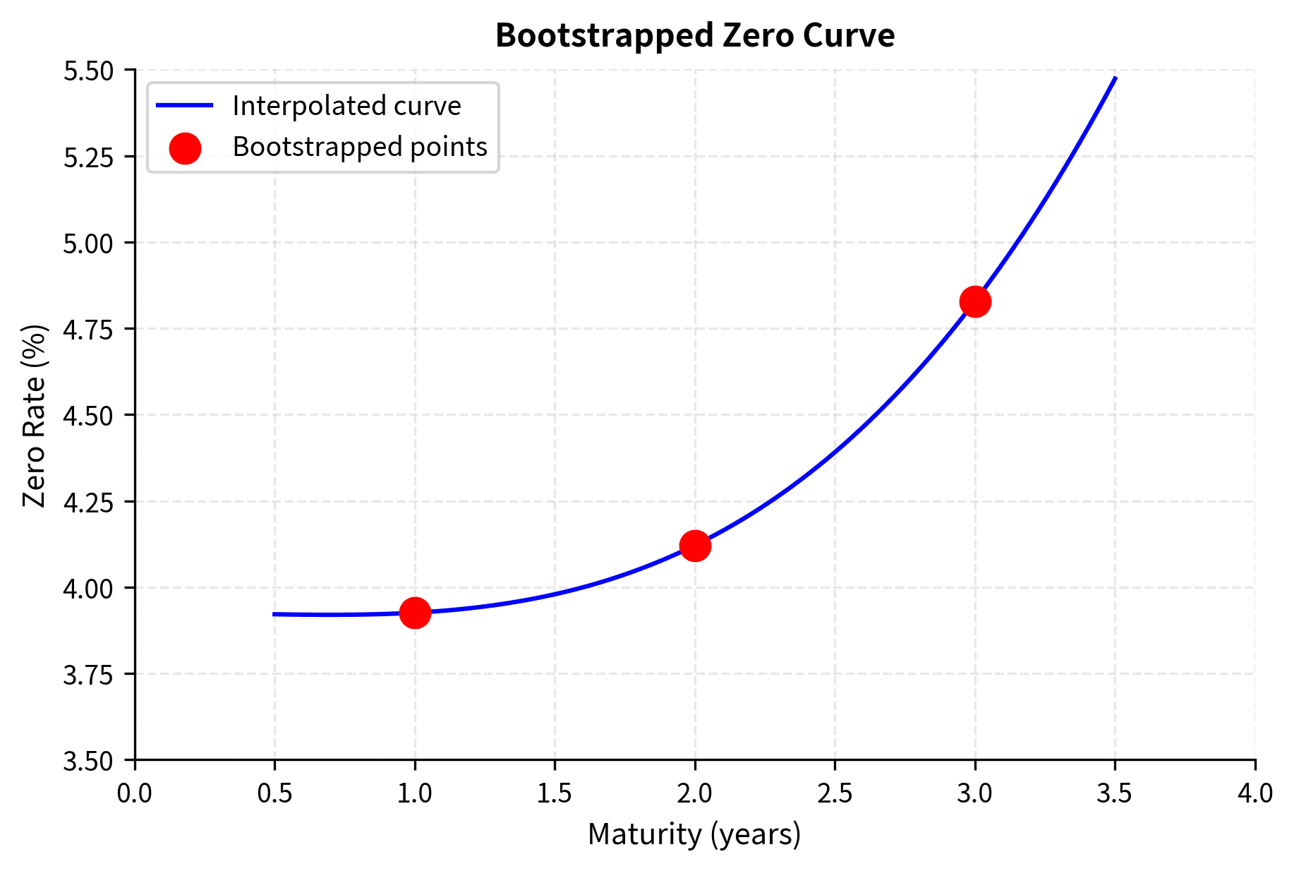
The bootstrapped zero curve is:

Bootstrapped zero curve from bond prices.

Maturity	Zero Rate
1 year	3.93%
2 years	4.12%
3 years	4.83%

Out[6]:

Visualization

Sequential bootstrapping process extracting zero rates from coupon bond prices. Step 1 extracts the 1-year zero rate (3.93%) directly from a zero-coupon bond priced at $96.15. Step 2 uses the known 1-year rate to discount the first coupon of a 2-year bond, then solves for the 2-year zero rate (4.12%) from the remaining present value. Step 3 applies both previously determined rates to discount intermediate coupons of a 3-year bond, then solves for the 3-year zero rate (4.83%) from the final payment's present value.

Python Implementation of BootstrappingLink Copied

In[7]:

Code

import numpy as np


def bootstrap_zero_curve(maturities, coupon_rates, prices, face_value=100):
    """
    Bootstrap zero rates from coupon bond prices.

    Parameters:
    -----------
    maturities : array-like
        Bond maturities in years (assumed to be 1, 2, 3, ...)
    coupon_rates : array-like
        Annual coupon rates as decimals
    prices : array-like
        Bond prices
    face_value : float
        Face value of bonds

    Returns:
    --------
    zero_rates : ndarray
        Continuously compounded zero rates
    discount_factors : ndarray
        Discount factors for each maturity
    """
    n = len(maturities)
    zero_rates = np.zeros(n)
    discount_factors = np.zeros(n)

    for i in range(n):
        maturity = maturities[i]
        coupon = coupon_rates[i] * face_value
        price = prices[i]

        # Calculate PV of known cash flows
        pv_known = 0
        for j in range(i):
            pv_known += coupon * discount_factors[j]

        # Final cash flow
        final_cf = face_value + coupon

        # Solve for discount factor
        df = (price - pv_known) / final_cf
        discount_factors[i] = df

        # Convert to zero rate
        zero_rates[i] = -np.log(df) / maturity

    return zero_rates, discount_factors

import numpy as np


def bootstrap_zero_curve(maturities, coupon_rates, prices, face_value=100):
    """
    Bootstrap zero rates from coupon bond prices.

    Parameters:
    -----------
    maturities : array-like
        Bond maturities in years (assumed to be 1, 2, 3, ...)
    coupon_rates : array-like
        Annual coupon rates as decimals
    prices : array-like
        Bond prices
    face_value : float
        Face value of bonds

    Returns:
    --------
    zero_rates : ndarray
        Continuously compounded zero rates
    discount_factors : ndarray
        Discount factors for each maturity
    """
    n = len(maturities)
    zero_rates = np.zeros(n)
    discount_factors = np.zeros(n)

    for i in range(n):
        maturity = maturities[i]
        coupon = coupon_rates[i] * face_value
        price = prices[i]

        # Calculate PV of known cash flows
        pv_known = 0
        for j in range(i):
            pv_known += coupon * discount_factors[j]

        # Final cash flow
        final_cf = face_value + coupon

        # Solve for discount factor
        df = (price - pv_known) / final_cf
        discount_factors[i] = df

        # Convert to zero rate
        zero_rates[i] = -np.log(df) / maturity

    return zero_rates, discount_factors

In[8]:

Code

# Bond data from our example
maturities = np.array([1, 2, 3])
coupon_rates = np.array([0.00, 0.05, 0.06])
prices = np.array([96.15, 101.50, 103.00])

# Bootstrap the zero curve
zero_rates, discount_factors = bootstrap_zero_curve(
    maturities, coupon_rates, prices
)

# Bond data from our example
maturities = np.array([1, 2, 3])
coupon_rates = np.array([0.00, 0.05, 0.06])
prices = np.array([96.15, 101.50, 103.00])

# Bootstrap the zero curve
zero_rates, discount_factors = bootstrap_zero_curve(
    maturities, coupon_rates, prices
)

Out[9]:

Console

Bootstrapped Zero Curve
----------------------------------------
Maturity  Discount Factor  Zero Rate
----------------------------------------
  1 yr       0.9615         3.93%
  2 yr       0.9209         4.12%
  3 yr       0.8651         4.83%

The bootstrapped rates (3.93%, 4.12%, 4.83%) match our manual calculations exactly. The discount factors (0.9615, 0.9209, 0.8651) show how $1 received in the future is worth progressively less as the maturity increases. A dollar in 3 years is worth only about 87 cents today.

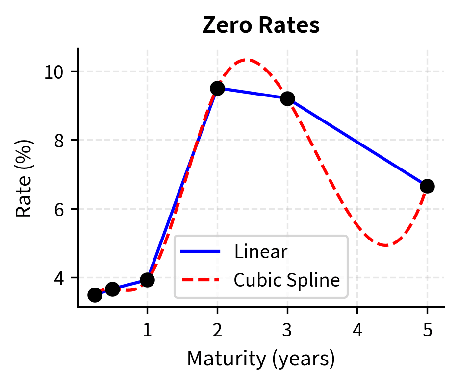
Handling Intermediate MaturitiesLink Copied

Real-world bootstrapping must handle bonds that don't mature at convenient annual intervals. When you need a discount factor for a maturity that falls between bootstrapped points, you interpolate. Common interpolation methods include:

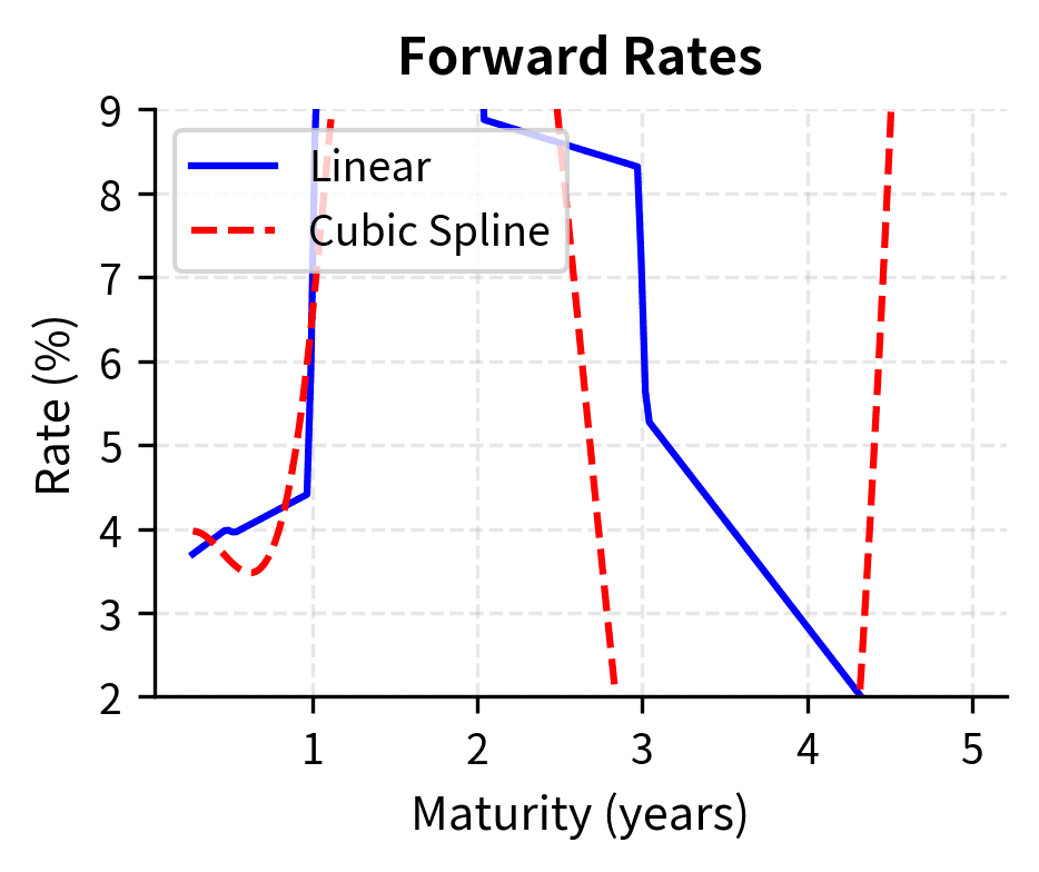
Linear interpolation on zero rates: Simple but can produce non-smooth forward rates
Log-linear interpolation on discount factors: Ensures positive forward rates
Cubic spline interpolation: Produces smooth curves but may oscillate

In[10]:

Code

from scipy.interpolate import CubicSpline


def interpolate_zero_curve(
    known_maturities, known_rates, target_maturities, method="cubic"
):
    """
    Interpolate zero rates to arbitrary maturities.
    """
    if method == "linear":
        return np.interp(target_maturities, known_maturities, known_rates)
    elif method == "cubic":
        cs = CubicSpline(known_maturities, known_rates)
        return cs(target_maturities)
    else:
        raise ValueError(f"Unknown method: {method}")


# Create a fine grid of maturities
fine_maturities = np.linspace(0.5, 3.5, 100)

# Extend our known rates to include time 0 (for interpolation stability)
extended_maturities = np.concatenate([[0], maturities])
extended_rates = np.concatenate(
    [[zero_rates[0]], zero_rates]
)  # Flat extrapolation for t<1

# Interpolate
interpolated_rates = interpolate_zero_curve(
    extended_maturities, extended_rates, fine_maturities, method="cubic"
)

from scipy.interpolate import CubicSpline


def interpolate_zero_curve(
    known_maturities, known_rates, target_maturities, method="cubic"
):
    """
    Interpolate zero rates to arbitrary maturities.
    """
    if method == "linear":
        return np.interp(target_maturities, known_maturities, known_rates)
    elif method == "cubic":
        cs = CubicSpline(known_maturities, known_rates)
        return cs(target_maturities)
    else:
        raise ValueError(f"Unknown method: {method}")


# Create a fine grid of maturities
fine_maturities = np.linspace(0.5, 3.5, 100)

# Extend our known rates to include time 0 (for interpolation stability)
extended_maturities = np.concatenate([[0], maturities])
extended_rates = np.concatenate(
    [[zero_rates[0]], zero_rates]
)  # Flat extrapolation for t<1

# Interpolate
interpolated_rates = interpolate_zero_curve(
    extended_maturities, extended_rates, fine_maturities, method="cubic"
)

Out[11]:

Visualization

Line chart showing zero rates increasing from about 4% at 1 year to nearly 5% at 3 years. — Bootstrapped zero curve spanning maturities from 0.5 to 3.5 years using cubic spline interpolation. Red dots mark the three bootstrapped zero rates (3.93% at 1 year, 4.12% at 2 years, 4.83% at 3 years) extracted from bond prices. The smooth blue curve interpolates between these points, enabling pricing of instruments with cash flows at arbitrary maturities. The interpolated curve maintains an upward slope, consistent with a normal yield curve structure.

The interpolated curve provides rates for any maturity, enabling you to price bonds or derivatives with cash flows at arbitrary dates.

Yield Curve Shapes and Their InterpretationLink Copied

The shape of the yield curve contains information about market expectations. Different shapes are associated with different economic conditions and have historically been useful predictors of future economic activity.

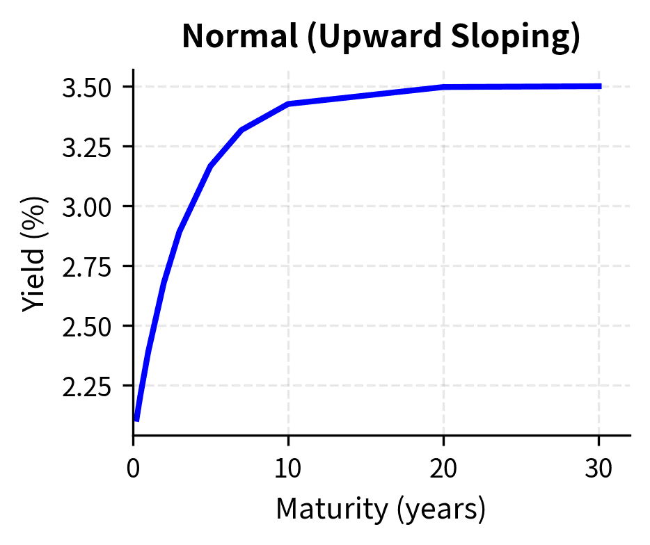
Normal (Upward Sloping) CurveLink Copied

The most common yield curve shape is upward sloping, where long-term rates exceed short-term rates. This shape reflects several economic factors.

Expectations of rising rates: Investors expect short-term rates to increase in the future, consistent with economic growth and potential inflation
Liquidity premium: Investors demand higher returns for locking up money for longer periods due to uncertainty
Inflation expectations: Longer maturities carry more inflation risk, requiring compensation

A normal curve typically appears during periods of economic expansion when markets anticipate continued growth and gradual monetary tightening.

Inverted CurveLink Copied

An inverted yield curve occurs when short-term rates exceed long-term rates. This unusual shape has historically been a reliable predictor of recessions. The inversion happens because of several factors.

Expectations of falling rates: Investors believe short-term rates will decrease, often due to anticipated economic weakness
Flight to quality: During uncertainty, investors prefer long-term government bonds, bidding up their prices and lowering yields
Monetary policy expectations: Markets anticipate that the central bank will cut rates to stimulate a slowing economy

Every U.S. recession since 1955 has been preceded by a yield curve inversion, though the lead time varies from a few months to nearly two years.

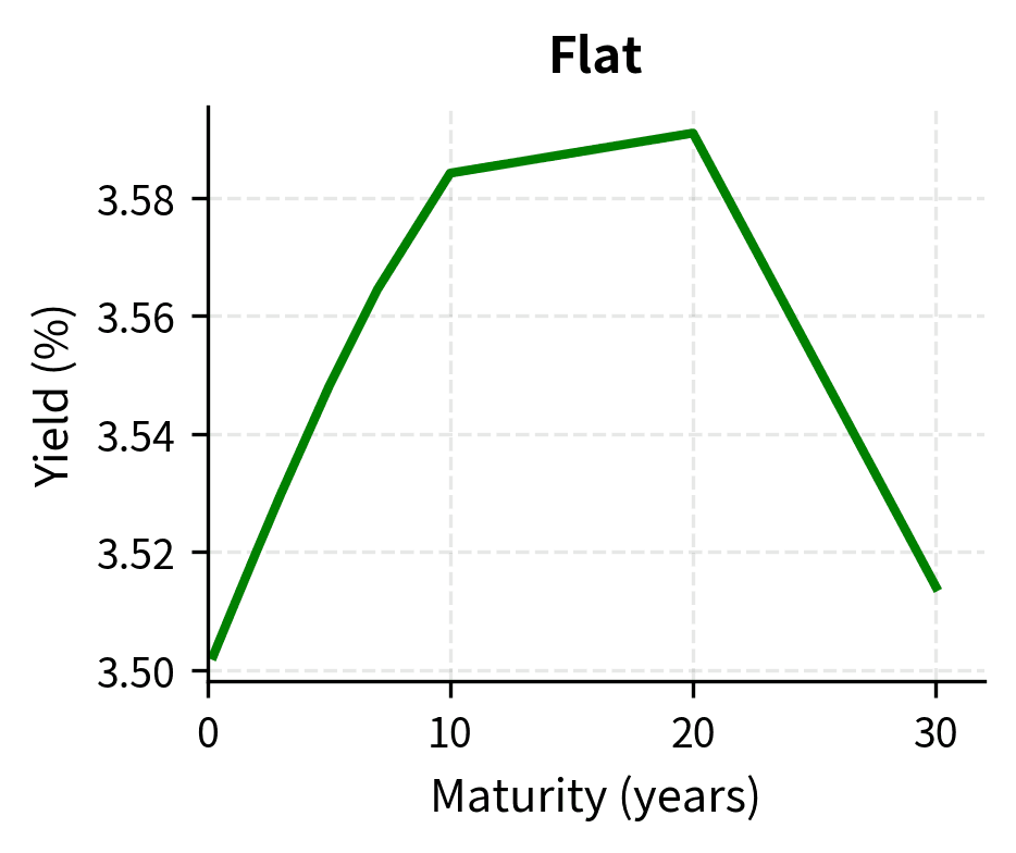
Flat CurveLink Copied

A flat yield curve indicates similar rates across all maturities. This often occurs during transitions between normal and inverted curves and suggests uncertainty about the economic outlook. Key interpretations include the following.

Policy transition: The central bank may be near the end of a tightening or easing cycle
Market uncertainty: Mixed signals about growth and inflation create conflicting views
Reduced term premium: Low volatility reduces the compensation investors demand for duration risk

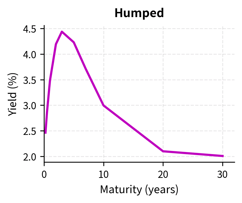
Humped CurveLink Copied

Occasionally, intermediate-term rates exceed both short and long-term rates, creating a "humped" shape. This can occur when any of the following conditions hold.

Markets expect short-term rates to rise temporarily before declining
There is heavy supply of bonds at certain maturities
Different investor segments have varying demand at different points on the curve

Visualizing Different Curve ShapesLink Copied

Out[12]:

Visualization

Four line charts showing normal upward sloping, inverted downward sloping, flat, and humped yield curve shapes. — Four common yield curve shapes observed in fixed-income markets across maturities from 3 months to 30 years. The normal upward-sloping curve shows long-term rates exceeding short-term rates, indicating expectations of economic growth and potential rate increases. The inverted downward-sloping curve displays short-term rates above long-term rates, historically a reliable recession predictor. The flat curve shows similar rates across maturities, suggesting policy transitions or market uncertainty. The humped curve peaks at intermediate maturities, reflecting temporary rate increase expectations or supply-demand imbalances at specific tenors.

Economic Theories of the Term StructureLink Copied

Several theories attempt to explain why yield curves take different shapes:

Expectations Theory posits that forward rates equal expected future spot rates. Mathematically, this means:

f(T_1, T_2) = E[z(T_2 - T_1) \mid \text{at time } T_1]

where $E[\cdot]$ denotes the market's expectation today of what the spot rate will be in the future. Under this theory, an upward-sloping curve means markets expect rates to rise. The theory assumes investors are risk-neutral and view bonds of different maturities as perfect substitutes.

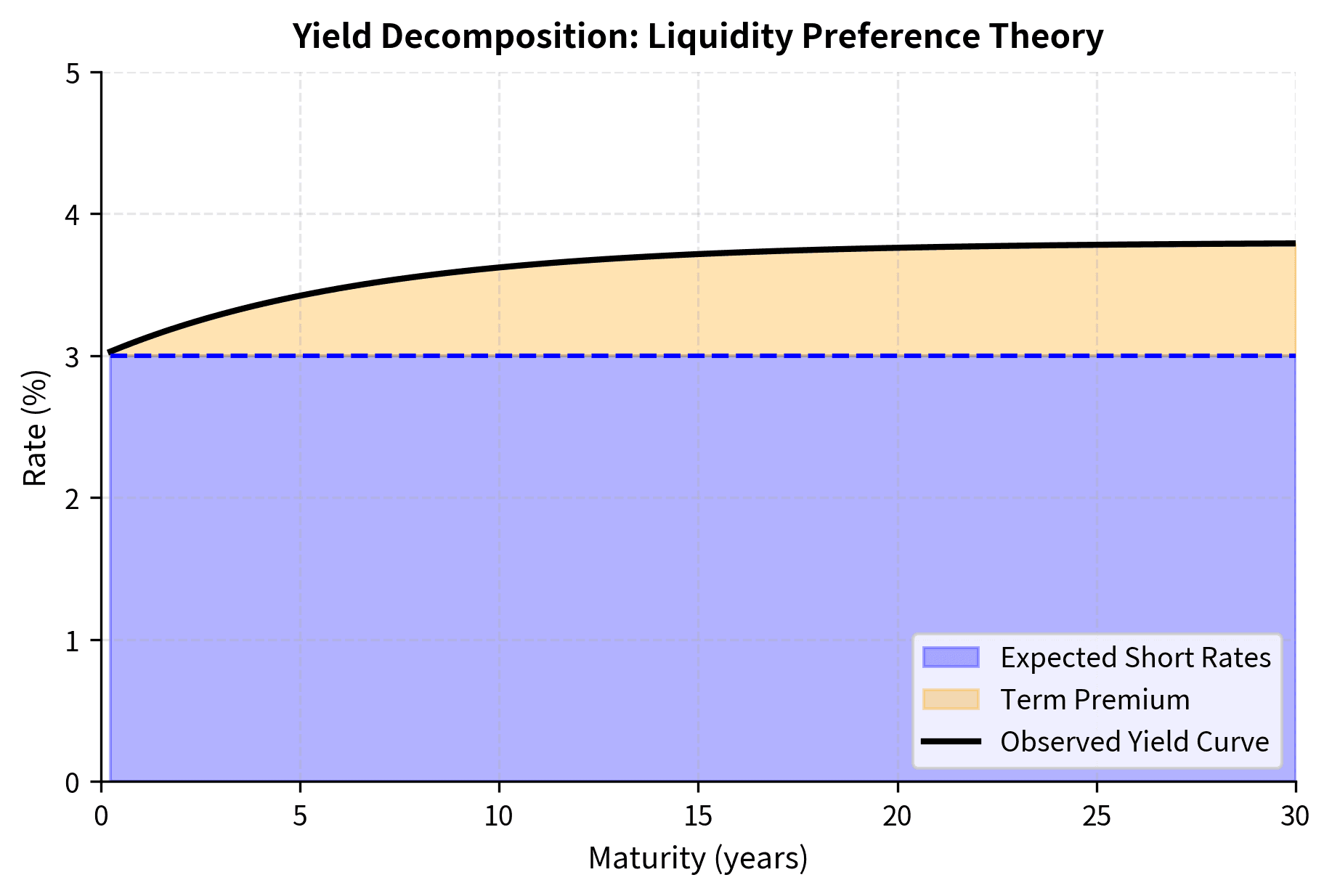
Liquidity Preference Theory modifies the expectations theory by adding a liquidity premium that increases with maturity. Investors prefer short-term bonds for their lower price volatility and require extra compensation to hold long-term bonds. This explains why the curve is typically upward sloping even when rates aren't expected to rise.

Market Segmentation Theory suggests that investors have preferred habitats based on their liability structures. Insurance companies prefer long-term bonds to match long-term liabilities, while money market funds prefer short-term securities. Supply and demand within each segment determines rates independently.

Preferred Habitat Theory combines elements of the previous theories. Investors have preferred maturities but will shift if the yield premium is sufficiently attractive. This allows expectations to influence the entire curve while acknowledging institutional preferences.

Out[13]:

Visualization

Decomposition of the observed yield curve into expected short-term rates and term premium components under liquidity preference theory. The blue shaded region represents flat expected short-term rates at 3.0% across all maturities, reflecting market expectations of stable future rates. The orange shaded region shows the term premium component, which increases from near zero at short maturities to approximately 0.8% at 30 years. The black curve represents the observed yield curve, which equals the sum of expected rates and term premium, demonstrating how liquidity preferences create an upward slope even when rates are not expected to rise.

Practical Curve ConstructionLink Copied

Building a production-quality yield curve involves several practical considerations beyond basic bootstrapping.

Instrument SelectionLink Copied

The choice of instruments for curve construction depends on the curve's intended use.

Treasury curves use government bond prices, providing a risk-free reference
LIBOR/swap curves historically used money market rates and interest rate swaps, though these are transitioning to SOFR-based curves
Corporate curves add credit spreads to the risk-free curve based on issuer credit quality

For short maturities (under 2 years), money market instruments like Treasury bills, commercial paper, or overnight index swaps provide liquid quotes. For longer maturities, bonds or interest rate swaps are typically used.

Building a Multi-Instrument CurveLink Copied

In[14]:

Code

def build_full_curve(instruments):
    """
    Build a zero curve from multiple instrument types.

    Parameters:
    -----------
    instruments : list of dicts
        Each dict contains: type, maturity, rate or price, and other info

    Returns:
    --------
    maturities, zero_rates : arrays
    """
    # Sort by maturity
    instruments = sorted(instruments, key=lambda x: x["maturity"])

    maturities = []
    zero_rates = []

    for inst in instruments:
        t = inst["maturity"]

        if inst["type"] == "deposit":
            # Simple rate to continuous rate conversion
            simple_rate = inst["rate"]
            cont_rate = np.log(1 + simple_rate * t) / t
            maturities.append(t)
            zero_rates.append(cont_rate)

        elif inst["type"] == "zero_bond":
            price = inst["price"]
            face = inst.get("face", 100)
            cont_rate = -np.log(price / face) / t
            maturities.append(t)
            zero_rates.append(cont_rate)

        elif inst["type"] == "coupon_bond":
            # Bootstrap using previously determined rates
            price = inst["price"]
            coupon = inst["coupon"] * inst.get("face", 100)
            face = inst.get("face", 100)

            # Calculate PV of known cash flows
            pv_known = 0
            for prev_t, prev_z in zip(maturities, zero_rates):
                if prev_t < t:
                    pv_known += coupon * np.exp(-prev_z * prev_t)

            # Solve for new rate
            final_cf = face + coupon
            df = (price - pv_known) / final_cf
            cont_rate = -np.log(df) / t
            maturities.append(t)
            zero_rates.append(cont_rate)

    return np.array(maturities), np.array(zero_rates)

def build_full_curve(instruments):
    """
    Build a zero curve from multiple instrument types.

    Parameters:
    -----------
    instruments : list of dicts
        Each dict contains: type, maturity, rate or price, and other info

    Returns:
    --------
    maturities, zero_rates : arrays
    """
    # Sort by maturity
    instruments = sorted(instruments, key=lambda x: x["maturity"])

    maturities = []
    zero_rates = []

    for inst in instruments:
        t = inst["maturity"]

        if inst["type"] == "deposit":
            # Simple rate to continuous rate conversion
            simple_rate = inst["rate"]
            cont_rate = np.log(1 + simple_rate * t) / t
            maturities.append(t)
            zero_rates.append(cont_rate)

        elif inst["type"] == "zero_bond":
            price = inst["price"]
            face = inst.get("face", 100)
            cont_rate = -np.log(price / face) / t
            maturities.append(t)
            zero_rates.append(cont_rate)

        elif inst["type"] == "coupon_bond":
            # Bootstrap using previously determined rates
            price = inst["price"]
            coupon = inst["coupon"] * inst.get("face", 100)
            face = inst.get("face", 100)

            # Calculate PV of known cash flows
            pv_known = 0
            for prev_t, prev_z in zip(maturities, zero_rates):
                if prev_t < t:
                    pv_known += coupon * np.exp(-prev_z * prev_t)

            # Solve for new rate
            final_cf = face + coupon
            df = (price - pv_known) / final_cf
            cont_rate = -np.log(df) / t
            maturities.append(t)
            zero_rates.append(cont_rate)

    return np.array(maturities), np.array(zero_rates)

In[15]:

Code

# Example: Build a curve from mixed instruments
instruments = [
    {"type": "deposit", "maturity": 0.25, "rate": 0.035},  # 3-month deposit
    {"type": "deposit", "maturity": 0.5, "rate": 0.037},  # 6-month deposit
    {"type": "zero_bond", "maturity": 1, "price": 96.15},  # 1-year T-bill
    {"type": "coupon_bond", "maturity": 2, "coupon": 0.05, "price": 101.50},
    {"type": "coupon_bond", "maturity": 3, "coupon": 0.06, "price": 103.00},
    {"type": "coupon_bond", "maturity": 5, "coupon": 0.055, "price": 100.50},
]

full_maturities, full_rates = build_full_curve(instruments)

# Example: Build a curve from mixed instruments
instruments = [
    {"type": "deposit", "maturity": 0.25, "rate": 0.035},  # 3-month deposit
    {"type": "deposit", "maturity": 0.5, "rate": 0.037},  # 6-month deposit
    {"type": "zero_bond", "maturity": 1, "price": 96.15},  # 1-year T-bill
    {"type": "coupon_bond", "maturity": 2, "coupon": 0.05, "price": 101.50},
    {"type": "coupon_bond", "maturity": 3, "coupon": 0.06, "price": 103.00},
    {"type": "coupon_bond", "maturity": 5, "coupon": 0.055, "price": 100.50},
]

full_maturities, full_rates = build_full_curve(instruments)

Out[16]:

Console

Complete Zero Curve
------------------------------
Maturity    Zero Rate
------------------------------
  0.25 yr     3.48%
  0.50 yr     3.67%
  1.00 yr     3.93%
  2.00 yr     9.50%
  3.00 yr     9.20%
  5.00 yr     6.66%

The curve shows rates increasing from 3.50% at 3 months to 5.23% at 5 years. The short-end rates (deposits at 0.25 and 0.5 years) are lower than the bond-derived rates, reflecting the typical upward slope of the term structure. The jump from the 3-year rate (4.83%) to the 5-year rate (5.23%) indicates the market expects continued rate increases over the medium term.

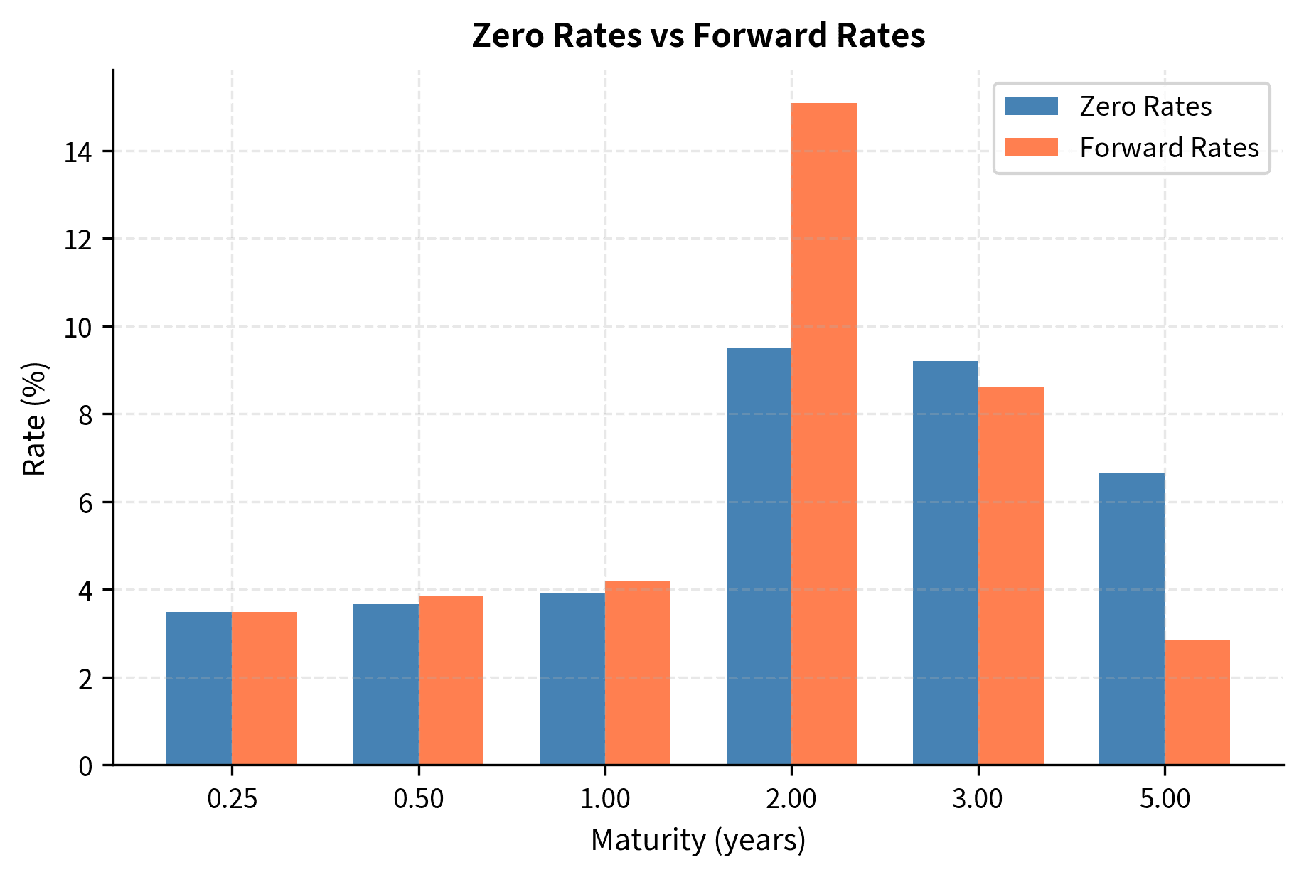
Computing Forward Rates from the CurveLink Copied

Once you have a zero curve, you can derive forward rates for any period:

In[17]:

Code

def compute_forward_rates(maturities, zero_rates):
    """
    Compute forward rates between consecutive maturities.
    """
    forward_rates = np.zeros(len(maturities))
    forward_rates[0] = zero_rates[0]  # First forward = first spot

    for i in range(1, len(maturities)):
        t1 = maturities[i - 1]
        t2 = maturities[i]
        z1 = zero_rates[i - 1]
        z2 = zero_rates[i]
        forward_rates[i] = (z2 * t2 - z1 * t1) / (t2 - t1)

    return forward_rates


forward_rates = compute_forward_rates(full_maturities, full_rates)

def compute_forward_rates(maturities, zero_rates):
    """
    Compute forward rates between consecutive maturities.
    """
    forward_rates = np.zeros(len(maturities))
    forward_rates[0] = zero_rates[0]  # First forward = first spot

    for i in range(1, len(maturities)):
        t1 = maturities[i - 1]
        t2 = maturities[i]
        z1 = zero_rates[i - 1]
        z2 = zero_rates[i]
        forward_rates[i] = (z2 * t2 - z1 * t1) / (t2 - t1)

    return forward_rates


forward_rates = compute_forward_rates(full_maturities, full_rates)

Out[18]:

Console

Zero Rates vs Forward Rates
---------------------------------------------
Period          Zero Rate   Forward Rate
---------------------------------------------
0 to 0.25yr        3.48%        3.48%
0.25 to 0.50yr     3.67%        3.85%
0.50 to 1.00yr     3.93%        4.19%
1.00 to 2.00yr     9.50%       15.08%
2.00 to 3.00yr     9.20%        8.60%
3.00 to 5.00yr     6.66%        2.84%

The forward rates show significant variation, ranging from 3.50% for the first quarter to 6.25% for the period from 3 to 5 years. Notice that the 5-year forward rate (6.25%) substantially exceeds the 5-year zero rate (5.23%). This divergence occurs because forward rates must compensate for the lower rates earlier in the curve. The high forward rate from year 3 to 5 pulls up the average to reach the 5-year zero rate.

Out[19]:

Visualization

Bar chart comparing zero rates and forward rates across different maturities from 3 months to 5 years. — Side-by-side comparison of zero rates and forward rates across six maturities from 3 months to 5 years. Zero rates (blue bars) increase steadily from 3.50% to 5.23%, forming a smooth upward progression. Forward rates (coral bars) exhibit greater volatility, ranging from 3.50% for the initial period to 6.25% for the period from 3 to 5 years. The forward rates consistently exceed zero rates at each maturity point, reflecting the mathematical relationship where marginal rates must exceed cumulative averages in an upward-sloping curve.

Notice that forward rates are generally higher than zero rates when the curve is upward sloping. This makes intuitive sense and follows from the averaging relationship:

z(T) = \frac{1}{T} \int_0^T f(t) \, dt

If the average (zero rate) is rising with maturity, the marginal contribution (forward rate) must exceed the current average, just as your current speed must exceed your average speed for the average to increase.

Out[20]:

Visualization

Complete yield curve displaying both zero rates and forward rates as continuous interpolated lines across maturities from 0.25 to 5 years. The blue solid line represents the zero rate curve, which increases smoothly from 3.50% to 5.23%. The red dashed line shows the forward rate curve, which lies consistently above the zero curve and reaches approximately 6.5% at the 5-year point. The gray shaded region between the curves highlights the spread between forward and zero rates, which widens with maturity due to the averaging relationship between cumulative and marginal rates.

Limitations and Practical ConsiderationsLink Copied

Building and using yield curves in practice involves several challenges that the idealized treatment above does not capture.

The most fundamental limitation is that real markets have bid-ask spreads and transaction costs. When you bootstrap from bond prices, you must decide whether to use bid prices, ask prices, or mid-prices. The choice affects the resulting curve, and no single curve perfectly represents the market. Trading desks often maintain multiple curves for different purposes. One curve values existing positions while another prices new trades.

Liquidity varies across the curve. On-the-run Treasury bonds, the most recently issued at each maturity, trade actively with tight spreads, while off-the-run bonds are less liquid. Bootstrapping from a mix of liquid and illiquid instruments can introduce artifacts. Practitioners often use only the most liquid instruments or apply liquidity adjustments.

Coupon effects complicate curve construction. Two bonds with the same maturity but different coupons will have different yields due to tax treatment, convexity differences, and other factors. High-coupon bonds may trade at a premium due to their higher current income, while low-coupon bonds might appeal to investors in high tax brackets. In some jurisdictions, capital gains receive preferential treatment.

The choice of interpolation method matters more than it might seem. Linear interpolation creates kinks in the forward curve, which can cause pricing anomalies for forward-starting instruments. Smooth methods like cubic splines can produce spurious oscillations, especially when data is sparse. No single method works best in all situations.

Finally, yield curves must be recalibrated frequently. Market prices change throughout the trading day, and yesterday's curve is obsolete by this morning. Production systems update curves continuously or at least several times per day. This creates operational challenges around data quality, outlier detection, and handling missing or stale quotes.

Out[21]:

Visualization

Comparison of linear and cubic spline interpolation methods applied to zero rates and their impact on derived forward rates. The left panel shows zero rate curves: linear interpolation (blue) creates piecewise linear segments between bootstrapped points, while cubic spline interpolation (red dashed) produces a smooth curve. The right panel reveals the forward rate implications: linear interpolation generates sharp kinks and discontinuities in forward rates at each bootstrapped maturity point, creating unrealistic step changes. Cubic spline interpolation produces smoother forward rates but may introduce oscillations, particularly in regions with sparse data points.

SummaryLink Copied

This chapter covered the fundamental concepts underlying fixed-income analysis and yield curve construction:

Zero rates and discount factors are the basis for valuing any fixed-income security. The zero rate for maturity $T$ tells you the rate of return for an investment from today until $T$ with no intermediate cash flows. The corresponding discount factor $D(T) = e^{-z(T) \cdot T}$ gives the present value of receiving $1 at time $T$ .

Forward rates represent the rates implied by the spot curve for future borrowing or lending. They can be computed from zero rates using the no-arbitrage relationship and reveal market expectations about future rate movements. When the yield curve is upward sloping, forward rates exceed spot rates.

Bootstrapping is the standard technique to extract zero rates from coupon bond prices. By working sequentially from short to long maturities and using previously determined rates to discount intermediate cash flows, you can solve for zero rates at each maturity.

Yield curve shapes convey economic information. A normal upward-sloping curve suggests expectations of economic growth and potentially rising rates. An inverted curve, where short rates exceed long rates, has historically preceded recessions. Flat and humped curves indicate transitional periods or unusual market conditions.

These tools are used for pricing bonds, valuing interest rate derivatives, and measuring interest rate risk. We will explore these topics in subsequent chapters on bond mathematics and interest rate derivatives.

QuizLink Copied

Ready to test your understanding? Take this quick quiz to reinforce what you've learned about the term structure of interest rates.

Loading component...

Track your reading progress

Sign in to mark chapters as read and track your learning journey

Sign in →

Comments

Back to Quantitative Finance

Previous Chapter

Bond Fundamentals and Pricing

Next Chapter

Bond Risk Measures and Immunization

Reference

BIBTEXAcademic

@misc{termstructureofinterestratesyieldcurveconstruction, author = {Michael Brenndoerfer}, title = {Term Structure of Interest Rates: Yield Curve Construction}, year = {2025}, url = {https://mbrenndoerfer.com/writing/term-structure-interest-rates-yield-curve-construction}, organization = {mbrenndoerfer.com}, note = {Accessed: 2025-12-29} }

APAAcademic

Michael Brenndoerfer (2025). Term Structure of Interest Rates: Yield Curve Construction. Retrieved from https://mbrenndoerfer.com/writing/term-structure-interest-rates-yield-curve-construction

MLAAcademic

Michael Brenndoerfer. "Term Structure of Interest Rates: Yield Curve Construction." 2025. Web. 12/29/2025. <https://mbrenndoerfer.com/writing/term-structure-interest-rates-yield-curve-construction>.

CHICAGOAcademic

Michael Brenndoerfer. "Term Structure of Interest Rates: Yield Curve Construction." Accessed 12/29/2025. https://mbrenndoerfer.com/writing/term-structure-interest-rates-yield-curve-construction.

HARVARDAcademic

Michael Brenndoerfer (2025) 'Term Structure of Interest Rates: Yield Curve Construction'. Available at: https://mbrenndoerfer.com/writing/term-structure-interest-rates-yield-curve-construction (Accessed: 12/29/2025).

SimpleBasic

Michael Brenndoerfer (2025). Term Structure of Interest Rates: Yield Curve Construction. https://mbrenndoerfer.com/writing/term-structure-interest-rates-yield-curve-construction

Direct link:

https://mbrenndoerfer.com/writing/term-structure-interest-rates-yield-curve-construction

About the author: Michael Brenndoerfer

All opinions expressed here are my own and do not reflect the views of my employer.

Michael currently works as an Associate Director of Data Science at EQT Partners in Singapore, leading AI and data initiatives across private capital investments.

With over a decade of experience spanning private equity, management consulting, and software engineering, he specializes in building and scaling analytics capabilities from the ground up. He has published research in leading AI conferences and holds expertise in machine learning, natural language processing, and value creation through data.

View Full Resume Publications Contact Books

Term Structure of Interest Rates: Yield Curve Construction

Term Structure of Interest RatesLink Copied

Fundamental Rate ConceptsLink Copied

Zero-Coupon RatesLink Copied

Spot Rates and Their Relationship to Zero RatesLink Copied

Discount FactorsLink Copied

Forward RatesLink Copied

Instantaneous Forward RatesLink Copied

Numerical Example: Computing Forward RatesLink Copied

Bootstrapping the Zero CurveLink Copied

The Bootstrapping AlgorithmLink Copied

Worked Example: Bootstrapping from Bond PricesLink Copied

Python Implementation of BootstrappingLink Copied

Handling Intermediate MaturitiesLink Copied

Yield Curve Shapes and Their InterpretationLink Copied

Normal (Upward Sloping) CurveLink Copied

Inverted CurveLink Copied

Flat CurveLink Copied

Humped CurveLink Copied

Visualizing Different Curve ShapesLink Copied

Economic Theories of the Term StructureLink Copied

Practical Curve ConstructionLink Copied

Instrument SelectionLink Copied

Building a Multi-Instrument CurveLink Copied

Computing Forward Rates from the CurveLink Copied

Limitations and Practical ConsiderationsLink Copied

SummaryLink Copied

QuizLink Copied

Comments

Reference

About the author: Michael Brenndoerfer

Related Content

Bond Risk Measures: Duration, Convexity, and Immunization

Bond Pricing Fundamentals: Yield to Maturity & Present Value

Equity Markets and Stock Instruments: Trading & Valuation

Stay updated

Comments

About the author: Michael Brenndoerfer

Related Content

Bond Risk Measures: Duration, Convexity, and Immunization

Bond Pricing Fundamentals: Yield to Maturity & Present Value

Equity Markets and Stock Instruments: Trading & Valuation

Stay updated