

Master continuous compounding, present value calculations, and differential equations. Essential tools for derivative pricing and financial modeling.
Choose your expertise level to adjust how many terms are explained. Beginners see more tooltips, experts see fewer to maintain reading flow. Hover over underlined terms for instant definitions.
Integral Calculus and Differential Equations
Calculus is the mathematics of continuous change, and finance is fundamentally about how value changes over time. While differential calculus, covered in the previous chapter, tells us the instantaneous rate of change, integral calculus answers the complementary question. Given how something is changing at each moment, what is its total accumulated effect? Differential equations combine both ideas, describing relationships between quantities and their rates of change that we must solve to understand the behavior of financial systems.
These tools are essential for quantitative finance. When interest rates compound continuously, we need integrals to compute total returns. When modeling asset prices that drift and diffuse over time, differential equations describe their dynamics. The Black-Scholes option pricing model, which we will derive in later chapters, is a partial differential equation. Understanding these foundations now will make those advanced models accessible rather than mysterious.
This chapter develops integral calculus and differential equations with a focus on financial applications. You will learn to compute accumulated returns, model continuous growth and decay processes, and see how these mathematical structures form the backbone of modern quantitative finance.
The Definite Integral as Accumulation
The definite integral captures the total accumulation of a quantity that changes continuously. To understand why this concept matters, imagine tracking the water flowing through a pipe. If you know the flow rate at every instant, the integral tells you the total volume of water that passed through over any time period. Similarly, in finance, if represents a rate of change at time (such as dollars flowing into an account per year, or the rate at which a liability grows), then the integral gives the total change from time to time .
Geometrically, the definite integral equals the signed area under the curve between and . Areas above the horizontal axis contribute positively, while areas below contribute negatively. This interpretation has direct financial meaning. If represents a continuous cash flow rate, the integral gives the total cash accumulated over the period. Positive cash flows add to your wealth, while negative cash flows (expenses or withdrawals) subtract from it.
The challenge, of course, is computing these areas precisely when the curve is not a simple geometric shape. This is where the formal definition through Riemann sums becomes essential, providing a rigorous foundation for calculating accumulated quantities even when the rate of change follows complex patterns.
The definite integral of a function from to is defined as the limit of Riemann sums:
where:
- : the interval of integration
- : number of subintervals (approaches infinity in the limit)
- : width of each subinterval
- : a sample point in the -th subinterval
- : value of at a sample point in the -th subinterval
- : approximate area of the -th rectangle
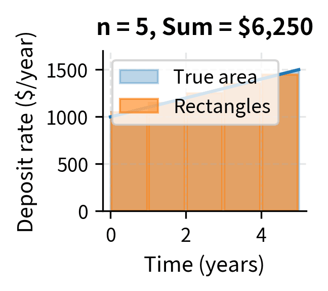
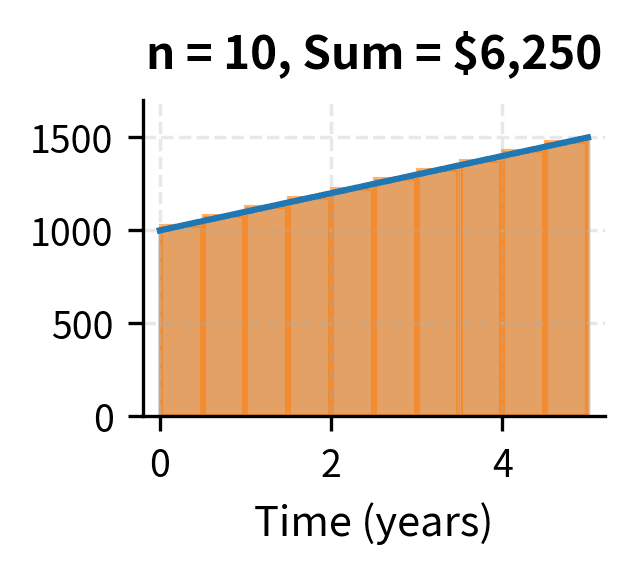
The Riemann sum approximates the area under the curve by summing rectangle areas. As , these rectangles become infinitely thin, and their sum converges to the exact area. This limit is the definite integral.
The intuition behind Riemann sums is straightforward: we approximate a complex shape using familiar ones. Just as ancient mathematicians approximated the area of a circle by inscribing polygons with ever more sides, we approximate the area under a curve by filling it with thin rectangles. Each rectangle has width and height determined by the function value at some point within that slice. The product gives the area of each rectangle, and summing all rectangles approximates the total area. As we use more rectangles (larger ), each rectangle becomes narrower ( shrinks), and the approximation becomes exact in the limit.

The Fundamental Theorem of Calculus connects differentiation and integration. It reveals that these two operations, which seem so different on the surface, are actually inverse operations. Differentiation finds instantaneous rates of change; integration accumulates total change. They are two sides of the same mathematical coin. If is an antiderivative of , meaning , then:
This theorem transforms the problem of computing integrals into finding antiderivatives, which is often more tractable than evaluating limits of sums directly. Rather than computing an infinite limit of rectangle sums, we can simply find a function whose derivative equals our integrand, then evaluate the difference at the endpoints. This is why antiderivative tables and integration techniques are so valuable: they provide shortcuts to what would otherwise require tedious limiting arguments.
A Financial Interpretation
Consider a savings account with a time-varying deposit rate measured in dollars per year. This rate might change because your income grows over time, or because you commit to increasing your contributions annually. Over a small time interval , you deposit approximately dollars—the rate times the duration. To find the total amount deposited from time to time , we must sum all these infinitesimal contributions, which is precisely what the integral computes:
If (you start depositing $1,000 per year and increase by $100 per year), then over 5 years:
You would deposit a total of $6,250 over the five-year period. Notice how the antiderivative captures both the base contribution () and the cumulative effect of the increasing contributions (). The Fundamental Theorem lets us compute this by simple evaluation rather than summing five years of daily deposits.
The numerical result confirms our analytical calculation. The scipy.integrate.quad function uses adaptive quadrature to compute definite integrals with high precision.
Continuous Compounding and the Exponential Function
The most important application of integral calculus in finance is understanding continuous compounding, a concept that underlies virtually all of modern quantitative finance. While the idea might seem abstract at first (no bank actually credits interest infinitely often), continuous compounding provides such mathematical elegance that it has become the standard framework for pricing derivatives, modeling interest rates, and valuing cash flows.
Recall from basic finance that discrete compounding with annual rate over periods gives a future value of:
This formula says: if you compound times per year, each compounding period credits interest at rate , and over years there are such periods. As the compounding frequency increases—moving from annual to quarterly to daily to hourly—this expression approaches a limit. Taking yields continuous compounding:
where:
- : future value of the investment
- : present value (initial investment)
- : Euler's number, the base of natural logarithms
- : annual interest rate (as a decimal)
- : time in years
The emergence of the exponential function here is no coincidence. It is the inevitable consequence of proportional growth. The exponential function emerges because, as compounding becomes continuous, the growth at each instant is proportional to the current value. If you have more money in your account, you earn more interest in the next instant, which means you have even more money, which earns even more interest. This self-reinforcing cycle, taken to its logical limit, produces exponential growth. The factor represents the cumulative effect of infinitely many infinitesimal compounding periods, each contributing a factor of that compounds multiplicatively.
This result connects directly to differential equations: the exponential function is the unique function that equals its own derivative (up to a constant), making it the natural solution to growth processes. This special property is why appears throughout mathematics and science whenever proportional growth or decay is involved.
Deriving Continuous Compounding from an Integral
Let's derive the continuous compounding formula using integral calculus, which reveals the deep connection between rates of change and accumulated growth. Suppose your account earns interest continuously at rate , and let denote the account value at time . The rate of change of your account value is proportional to the current value: the more you have, the faster it grows.
where:
- : account value at time
- : instantaneous rate of change of account value
- : continuous interest rate
- : interest earned per unit time, proportional to current balance
This equation captures compound interest: your wealth grows at a rate proportional to itself. This is a differential equation, and solving it will reveal the exponential function as the unique answer. To solve it, we use a technique called separation of variables. We rearrange the equation so that all terms involving are on one side and all terms involving are on the other:
Integrating both sides:
where is the constant of integration. Exponentiating both sides:
Setting and letting be the initial value:
Therefore, , and the solution is:
This derivation shows why the exponential function appears throughout finance: it is the natural solution to proportional growth. Whenever we have a quantity whose rate of change is proportional to its current value, whether that's money earning interest, a stock price drifting upward, or a liability accumulating over time, the exponential function provides the answer.
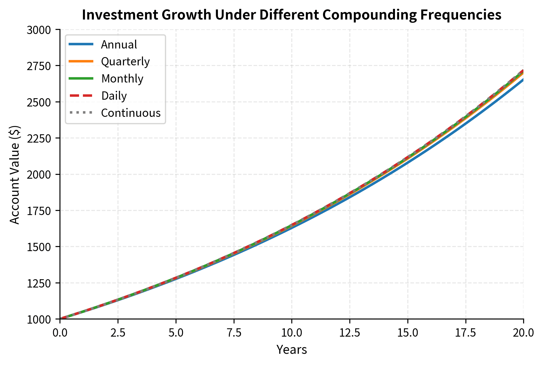
The plot demonstrates that as compounding frequency increases, the investment value approaches the continuous compounding limit. After 20 years at 5% interest, the final values illustrate the practical differences:
While the difference between daily and continuous compounding is small (about $0.36 on a $1,000 investment over 20 years), continuous compounding provides mathematical elegance that simplifies many calculations in quantitative finance.
Integration Techniques for Finance
Several integration techniques appear frequently in financial calculations. Mastering these methods is essential because real-world financial models rarely yield to simple antiderivatives. We focus on those most relevant to quantitative applications, building from the basic techniques to more sophisticated approaches used in derivative pricing.
Integration by Substitution
Integration by substitution reverses the chain rule of differentiation, allowing us to simplify integrals by changing variables. The core insight is that a complex integrand might become simple under the right transformation. If is a differentiable function and is continuous, then:
where .
The power of substitution lies in recognizing when an integrand contains a function and its derivative: the signature of the chain rule applied in reverse. When we spot this pattern, we can simplify the integral by treating the inner function as a new variable.
Consider pricing a bond with continuous coupon payments where the coupon rate decays exponentially. This structure might arise when modeling a company whose cash flows are expected to decline over time. If the coupon rate at time is and the discount factor is , we need to compute the present value of this decaying stream of payments:
where:
- : initial coupon rate at
- : decay rate of the coupon (how fast it decreases)
- : risk-free discount rate
- : maturity time
The present value of coupons from to is:
Here we used the property that to combine the exponentials. Now we apply substitution with , so :
The factor in the denominator represents the combined effect of discounting and coupon decay, as both reduce the present value of future payments. Discounting at rate makes future dollars worth less today, and decay at rate means those future dollars are smaller to begin with. The sum captures both effects simultaneously. The term approaches 1 as , giving the perpetuity value . This limiting case represents a bond that pays forever, where coupons decay but never quite reach zero.
Integration by Parts
Integration by parts reverses the product rule, enabling us to integrate products of functions by transferring the derivative from one factor to another. This technique is especially valuable when one function becomes simpler upon differentiation while the other has a known antiderivative. For functions and :
where:
- : a function chosen to simplify when differentiated
- : a function whose antiderivative is known
- : the differential of
- : the differential of
The strategy is to choose and so that is simpler than the original integral. A useful mnemonic for choosing is LIATE (Logarithmic, Inverse trigonometric, Algebraic, Trigonometric, Exponential), which suggests the order of preference for what to differentiate.
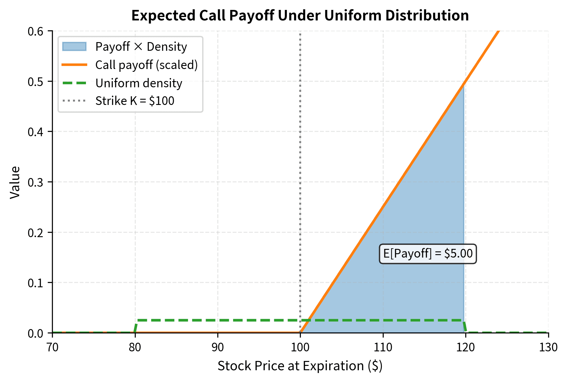
This technique is important when integrating products, especially in option pricing where payoffs multiply probability densities. When computing expected values, we often encounter integrals of the form , where is some probability density.
Consider computing the expected payoff of a call option under a uniform distribution (a simplified model for illustration). If the stock price at expiration is uniformly distributed on with strike , the expected payoff is:
This integral is straightforward:
The Gaussian Integral
The Gaussian integral is fundamental to quantitative finance because normal distributions appear throughout risk modeling and option pricing. Whenever we assume returns are normally distributed (an assumption underlying much of modern portfolio theory and option pricing), we encounter integrals involving the exponential of a quadratic. The basic Gaussian integral states:
This result, that integrating a bell curve over all real numbers yields exactly , is not obvious and requires sophisticated techniques to prove. The appearance of , usually associated with circles, shows connections in mathematics between seemingly unrelated concepts.
More generally, for the standard normal density:
This integral equals 1 because it represents the total probability under the standard normal density. Probability distributions must integrate to unity by definition. The factor is precisely the normalization constant that ensures this property.
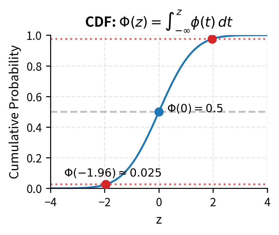
The cumulative distribution function of the standard normal:
where:
- : cumulative distribution function (CDF) of the standard normal distribution
- : upper limit of integration, representing the number of standard deviations
- : dummy variable of integration
- : the standard normal probability density function
has no closed-form expression but is tabulated and computed numerically. Despite appearing simple, this integral cannot be evaluated using elementary functions, which has practical implications. It appears directly in the Black-Scholes formula for option pricing, where call and put prices are expressed in terms of and . This is why option pricing software and spreadsheets must rely on numerical approximations or lookup tables for the normal CDF.
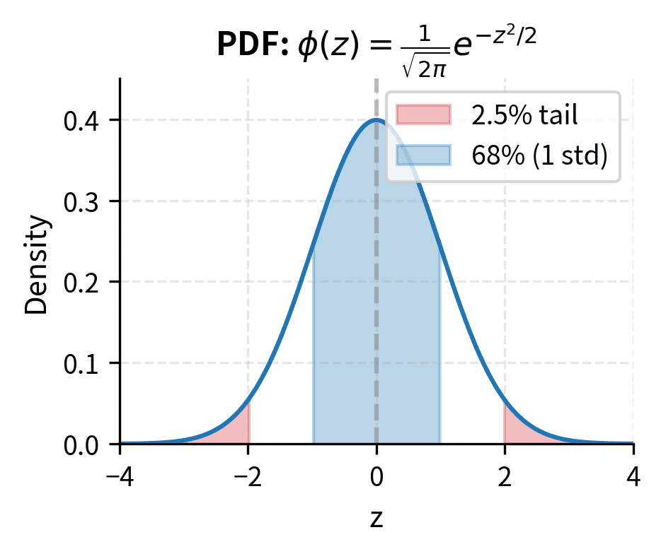
These probabilities have direct financial interpretations: means there is about a 2.3% probability that a standard normal variable falls below standard deviations, corresponding to extreme negative returns.
Present Value and the Yield Curve
An important application of integration in finance is computing present values when interest rates vary over time. In the real world, interest rates are not constant. Short-term rates typically differ from long-term rates, creating what traders call the yield curve. This curve describes the relationship between interest rates and maturities, and integrating along it determines how future cash flows are discounted.
Understanding how to discount with time-varying rates is essential because the shape of the yield curve affects everything from bond prices to mortgage rates to the value of long-dated derivatives. An upward-sloping curve (short rates lower than long rates) has different implications than an inverted curve, and our integration framework captures these differences precisely.
Continuous Discounting with Time-Varying Rates
When the instantaneous interest rate varies with time, we can no longer simply apply the formula because there is no single rate to use. Instead, we must account for the rate prevailing at each instant along the path from today to the future payment date. The discount factor from time to time accumulates all these instantaneous rates through integration:
where:
- : discount factor from time to time
- : instantaneous (spot) interest rate at time
- : dummy variable of integration representing time
- : accumulated interest over the period
This formula generalizes the constant-rate discount factor . The integral accumulates the instantaneous rates along the yield curve, and the exponential of the negative of this sum gives the discount factor. Notice that the integral is inside the exponential: we are not averaging the discount factors, but rather accumulating the rates and then applying a single exponential. This distinction matters because compounding is multiplicative, not additive.
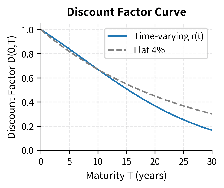
The discount factor represents the present value of $1 to be received at time . When rates are positive, , reflecting that future money is worth less than present money.
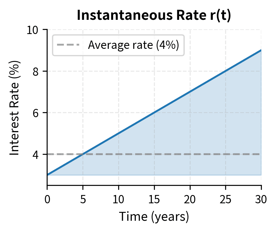
Consider a yield curve where the instantaneous rate starts at 3% and increases linearly to 5% over 10 years:
This upward-sloping curve reflects the common situation where investors demand higher rates for longer-term commitments, perhaps due to inflation uncertainty or preference for liquidity. The discount factor for a 10-year cash flow is:
Computing the integral:
Therefore:
A cash flow of $1,000 in 10 years has a present value of approximately $670.32. Notice that the effective discount is stronger than if we had used the average rate of 4%: gives the same answer, but only because of the linear form of our rate function. For more complex yield curves, the integral approach is essential.
The discount factors decrease with maturity, and the decline accelerates because the higher rates at longer maturities compound their effect.
Pricing a Bond with Continuous Coupons
Consider a bond paying continuous coupon at rate per year on a principal of , maturing at time . While real bonds pay discrete coupons, the continuous approximation simplifies analysis and closely approximates bonds with frequent payments. The present value combines the stream of coupons and the principal repayment:
where:
- : present value of the bond
- : continuous coupon rate (per year)
- : principal (face value)
- : maturity time
- : discount factor from time to time
The first term captures the present value of all coupon payments: at each instant , the bond pays per year, and this payment is discounted back to today using . The second term is the present value of the principal repayment at maturity.
With our upward-sloping yield curve:
The bond trades slightly below par because the coupon rate (4%) is below the average yield curve rate over the bond's life.
Ordinary Differential Equations in Finance
Differential equations describe relationships between quantities and their rates of change. Unlike algebraic equations that tell us what value a quantity takes, differential equations tell us how a quantity evolves, a different and more dynamic perspective. In finance, they model how portfolios, prices, and economic variables evolve over time, capturing the dynamic nature of markets and economies.
Differential equations encode rules of change that, when solved, reveal the trajectory of a system. If we know that interest rates revert toward a long-term mean, or that a portfolio grows proportionally to its value plus deposits, we can express these dynamics as differential equations and solve for the resulting paths.
First-Order Linear ODEs
A first-order linear ordinary differential equation has the form:
The term "first-order" means the equation involves only the first derivative of , not higher derivatives. "Linear" means and its derivative appear only to the first power and are not multiplied together. These constraints ensure the existence of a systematic solution method.
The general solution uses an integrating factor :
where:
- : the unknown function we are solving for
- : coefficient function multiplying
- : forcing function (the non-homogeneous term)
- : integrating factor that makes the left side a perfect derivative
- : constant of integration, determined by initial conditions
The integrating factor works because multiplying by converts the left side into , allowing direct integration. This technique appears frequently in differential equations. By multiplying through by just the right function, we transform a seemingly intractable equation into one we can solve by straightforward integration.
Example: Portfolio Growth with Continuous Deposits
Suppose you have a portfolio earning continuous return and you make continuous deposits at rate per year. This models a retirement account where you contribute regularly while earning investment returns. The portfolio value satisfies:
This equation says: the rate of change of your portfolio equals the investment return (, proportional to what you have) plus your deposits (, a constant flow). This is a first-order linear ODE with and . The integrating factor is .
Multiplying both sides by :
The left side is the derivative of :
This is the key insight: what looked like two separate terms is actually a single derivative. Now we can integrate directly:
With initial condition :
The solution is:
The first term represents growth of the initial investment, while the second represents accumulated deposits with their earned interest. This decomposition is intuitive. Your wealth at any time is the sum of what your original stake has grown to, plus what your contributions have accumulated.
The factor has a useful interpretation: it equals the perpetuity value of deposits at rate discounted at rate . If you deposited forever, the present value of all those deposits would be . The expression represents the growth factor for continuous deposits: at this is zero (no deposits accumulated yet), and it grows exponentially over time.
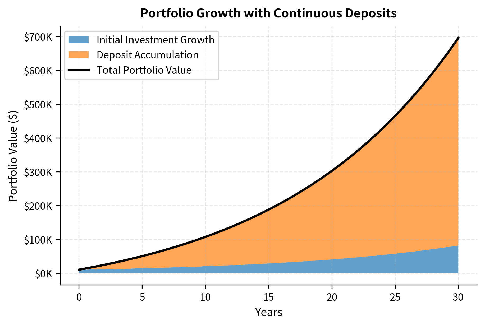
The power of compounding is evident: starting with $10,000 and depositing $6,000 per year, the portfolio grows to over $600,000 after 30 years, with investment gains far exceeding the total contributions.
Numerical Solution of ODEs
When differential equations lack closed-form solutions, numerical methods are essential. Many realistic financial models, especially those with time-varying parameters, nonlinear terms, or complex interactions, cannot be solved analytically. The scipy.integrate.odeint function implements efficient numerical solvers that approximate solutions to arbitrary precision.
Example: Mean-Reverting Interest Rates
The Vasicek model describes interest rates that revert to a long-term mean, capturing an important empirical feature of interest rate behavior: rates don't wander arbitrarily high or low but tend to fluctuate around some equilibrium level determined by economic fundamentals:
where:
- : instantaneous interest rate at time
- : speed of mean reversion (larger values mean faster reversion)
- : long-term mean interest rate
- : deviation from the long-term mean
The model reflects that interest rates don't wander arbitrarily but are pulled back toward equilibrium levels by market forces. Central banks target inflation and employment, creating pressure toward certain rate levels. Market forces and arbitrage prevent rates from staying too far from fundamentals for too long. When , the derivative is negative (rate decreases); when , the derivative is positive (rate increases). The parameter controls how strongly rates are pulled back: larger means faster reversion.
This ODE has an analytical solution, but let's solve it numerically to demonstrate the technique:
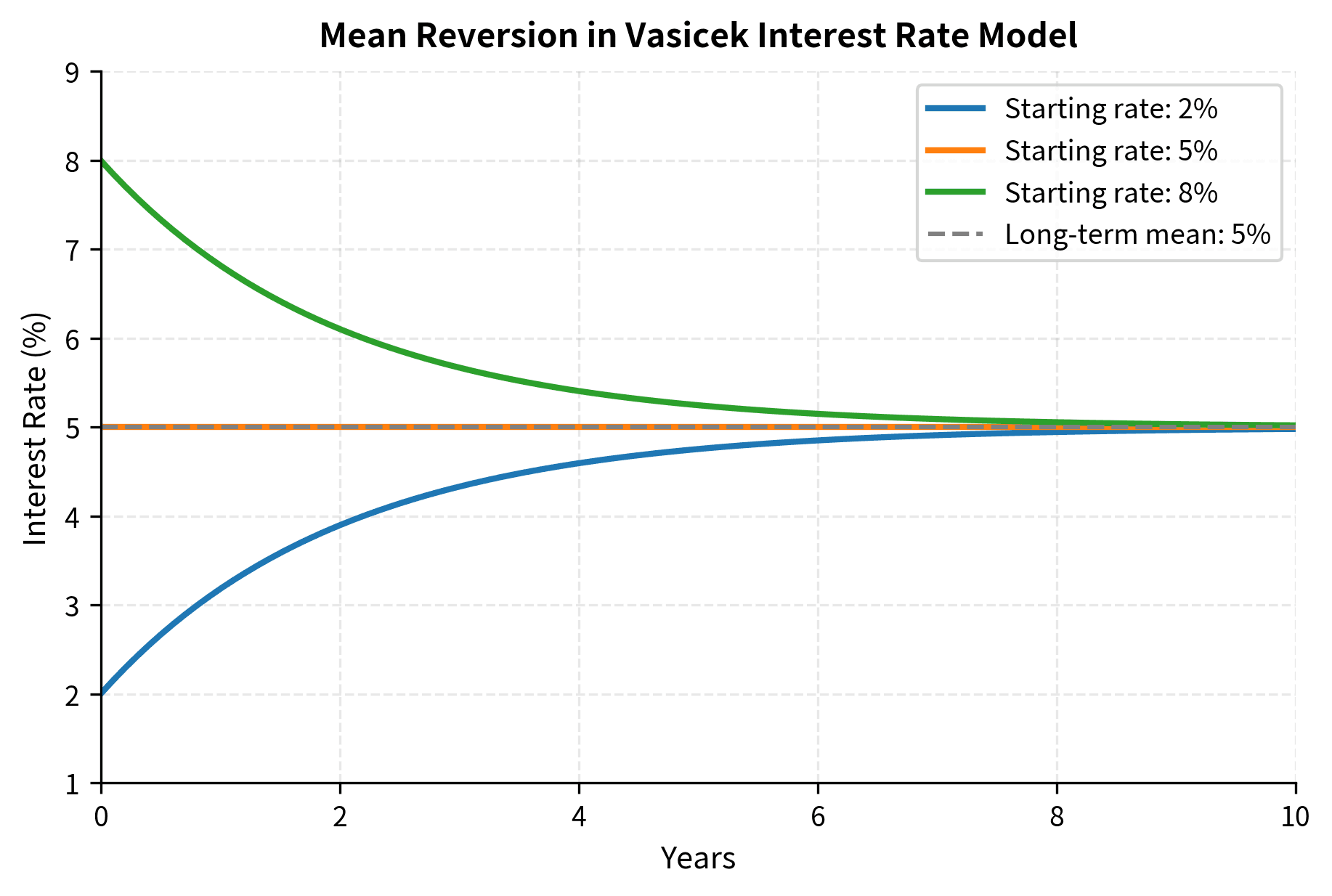
The mean reversion parameter implies a half-life of years: after about 1.4 years, the rate has moved halfway toward the long-term mean.
Separation of Variables and Financial Models
Separation of variables is a technique for solving certain differential equations by isolating each variable on opposite sides of the equation. The method works when we can algebraically rearrange an equation so that all terms involving the dependent variable (and its differential) appear on one side, while all terms involving the independent variable appear on the other. We can then integrate both sides independently. Many fundamental financial models yield to this approach.
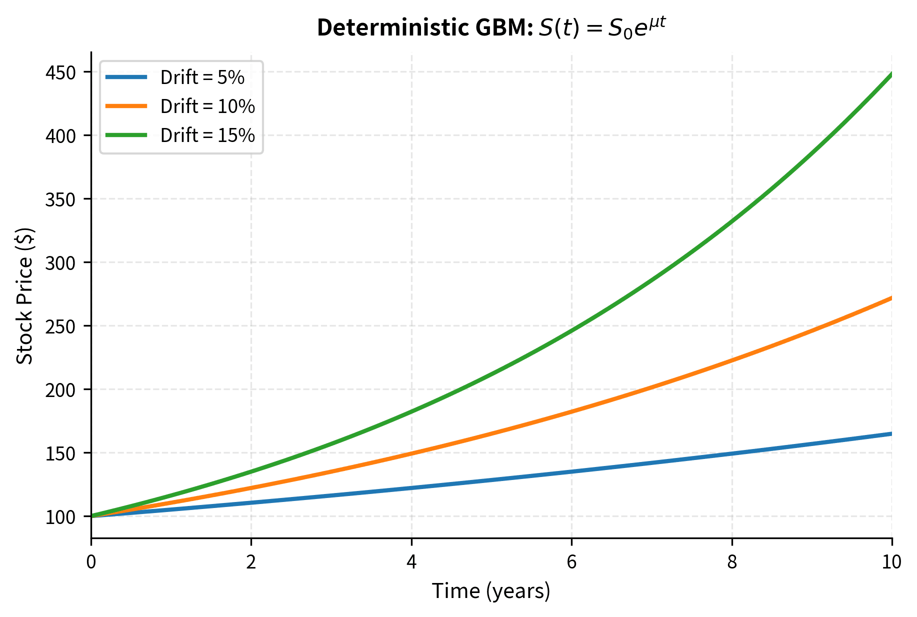
Geometric Brownian Motion (Deterministic Part)
The deterministic component of the geometric Brownian motion model for stock prices is:
where:
- : stock price at time
- : drift rate (expected return per unit time)
- : rate of change of stock price
The proportionality to means percentage changes are constant: a $100 stock and a $200 stock both grow at the same percentage rate , which matches how investors think about returns. This is essential: investors care about percentage returns, not dollar returns. A $10 gain on a $100 stock (10% return) is very different from a $10 gain on a $1000 stock (1% return). Separating variables:
Integrating:
This exponential growth model underlies the random component that we add in stochastic calculus (covered in later chapters). The deterministic drift provides the expected path around which prices fluctuate. In reality, stock prices don't follow smooth exponential curves; they jump around unpredictably. But this deterministic solution gives us the trend: the average behavior around which actual prices oscillate.
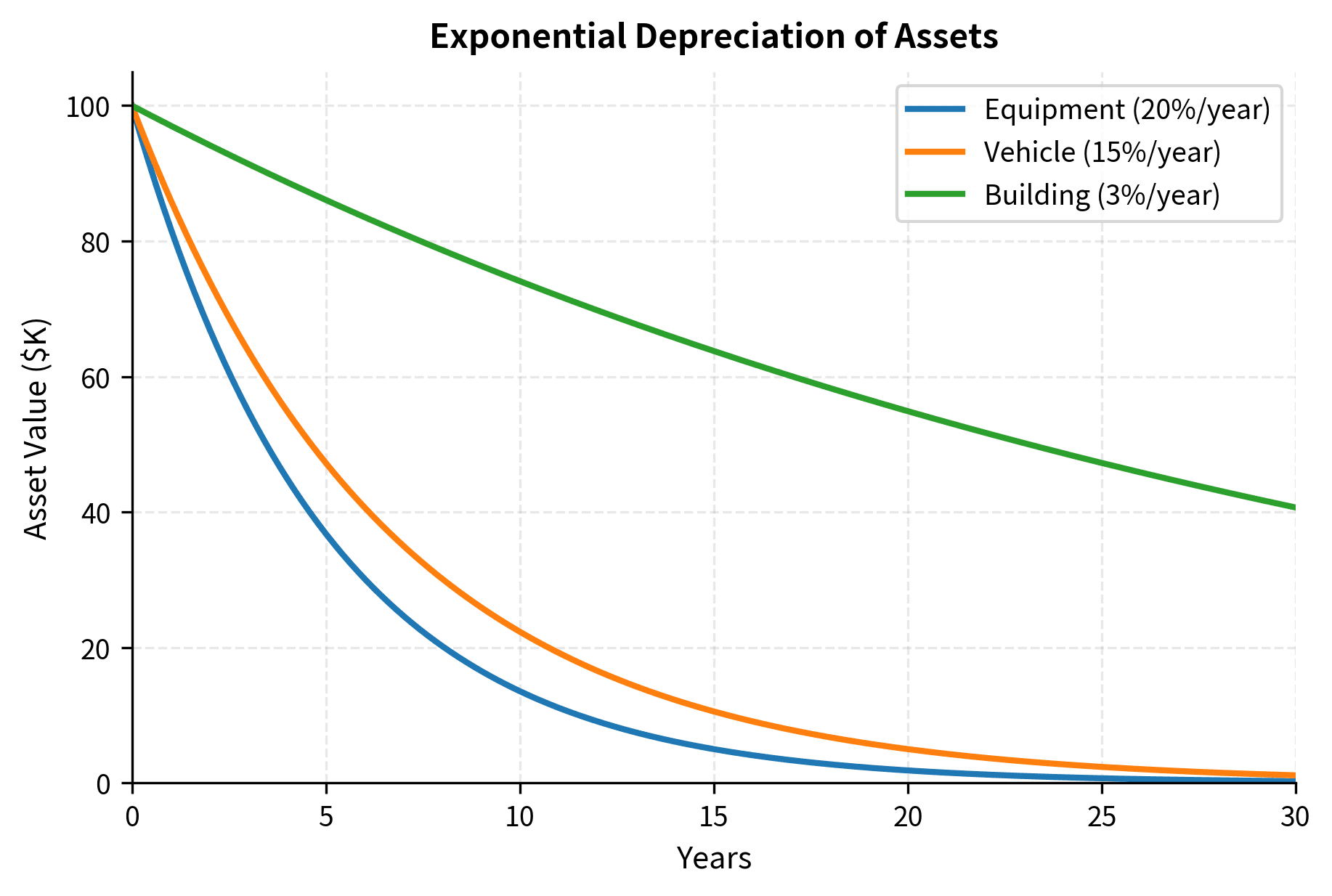
Decay Models: Asset Depreciation
Physical assets depreciate over time. A simple model assumes depreciation proportional to current value:
where:
- : asset value at time
- : depreciation rate (fraction of value lost per unit time)
- : negative because value decreases over time
The proportional model implies that newer (more valuable) assets lose more dollar value per year, but all assets lose the same percentage of value. A new car worth $30,000 might lose $4,500 in its first year (15%), while a five-year-old car worth $15,000 loses $2,250 (also 15%). The percentage rate is constant even though the dollar amounts differ. The solution is:
where is the initial asset value at .
The asset value decays exponentially, with half-life . The half-life formula follows directly from solving , which gives and thus . This is the time required for an asset to lose half its value.
The Logistic Equation: Bounded Growth
Not all financial quantities grow exponentially forever. Market saturation, resource constraints, and competition impose limits. A new product might grow rapidly when few competitors exist and many potential customers remain, but growth slows as the market becomes crowded. The logistic differential equation models growth that slows as it approaches a carrying capacity:
where:
- : the quantity being modeled (population, market share, adoption rate)
- : time
- : intrinsic growth rate (growth rate when is small)
- : carrying capacity (maximum sustainable value)
- : saturation factor that approaches zero as approaches
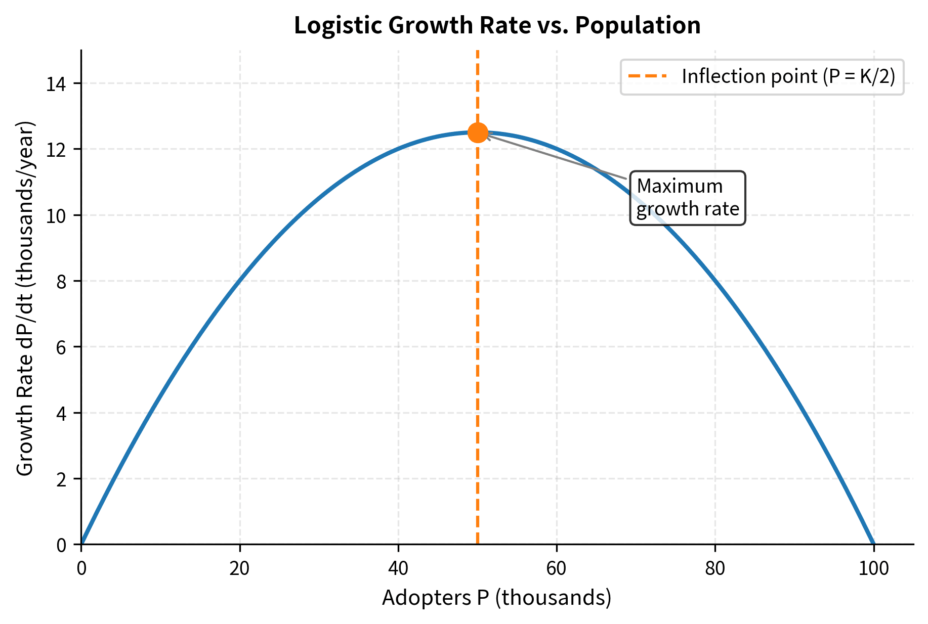
The term explains this model's behavior. When is small compared to , this factor is close to 1, and growth is approximately exponential at rate . As grows and approaches , the factor shrinks toward zero, progressively slowing growth. At exactly , growth stops entirely: the system has reached its carrying capacity.
When is small relative to , growth is approximately exponential: . As approaches , the factor approaches zero, slowing growth. At , growth stops entirely.
The logistic equation has an analytical solution:
where:
- : quantity at time
- : initial quantity at
- : carrying capacity
- : intrinsic growth rate
- : ratio determining how far the initial value is from capacity
The solution exhibits S-shaped (sigmoid) behavior due to the interplay between exponential growth (the term) and saturation (the denominator approaching 1 as ). Early on, when is small, the exponential term dominates and growth is nearly exponential. As the denominator stabilizes near 1 (when the exponential term becomes negligible), asymptotically approaches .
This S-shaped curve appears in technology adoption, market penetration, and the spread of financial products. Think of smartphones: early adopters bought them quickly, creating rapid initial growth. As more people owned phones, the remaining market shrank, and growth slowed. Eventually, the market reached saturation.
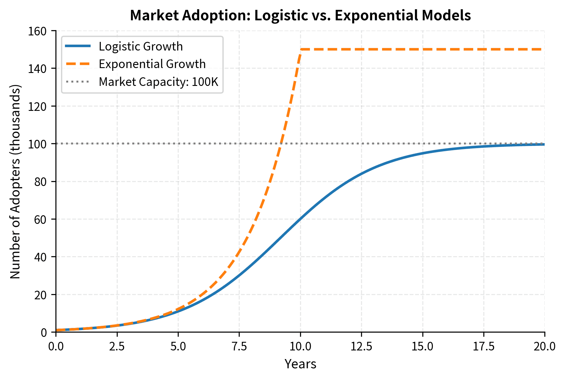
The logistic model shows rapid initial growth that slows as the market saturates. The inflection point (fastest growth) occurs when :
Connecting to Continuous-Time Finance
The mathematical tools developed in this chapter form the foundation for continuous-time financial models. This section previews how these concepts connect to more advanced topics.
The Black-Scholes PDE
The Black-Scholes equation for option pricing is a partial differential equation:
where:
- : option value (function of and )
- : time
- : underlying asset price
- : volatility of the underlying asset
- : risk-free interest rate
- : rate of change of option value with respect to time (theta)
- : rate of change of option value with respect to asset price (delta)
- : second derivative with respect to asset price (gamma)
This PDE combines ideas from this chapter.
The partial derivatives describe how option value changes with time and stock price . Unlike ordinary differential equations where we have one independent variable, here depends on both and , requiring partial derivatives to capture how responds to changes in each variable separately.
The equation structure resembles a diffusion equation with drift. The term involving the second derivative () captures how uncertainty diffuses through the option value. The first derivative term () captures drift.
Solving the PDE requires integration techniques and boundary conditions. Specifically, we need the option payoff at expiration as a boundary condition and use the integration methods we've developed to work backward to find today's price.
The derivation and solution of this equation will be covered in detail in later chapters, and recognizing its structure as a differential equation prepares you for what follows.
Stochastic Differential Equations
Financial models include randomness. A stochastic differential equation (SDE) generalizes the ODEs in this chapter by adding a random component:
where:
- : infinitesimal change in asset price
- : current asset price
- : drift rate (expected return)
- : volatility (standard deviation of returns)
- : infinitesimal time increment
- : increment of a Wiener process (Brownian motion)
- : deterministic drift component
- : random diffusion component
The first term () is the deterministic drift we analyzed earlier in this chapter, representing the expected growth of the stock price over time. The second term () adds random fluctuations driven by a Wiener process , which is a mathematical model of Brownian motion. These random shocks cause the stock price to fluctuate unpredictably while maintaining an overall drift. Solving SDEs requires stochastic calculus, which extends the integration techniques from this chapter to handle these random components.
Present Value as an Expectation
Under risk-neutral pricing, the price of a derivative equals the discounted expected payoff:
Computing this expectation involves integrating the payoff function against the probability density:
where:
- : present value of the derivative
- : risk-free interest rate
- : time to expiration
- : discount factor
- : payoff function (e.g., for a call option)
- : possible terminal stock price
- : risk-neutral probability density of the terminal stock price
- : expected payoff under the risk-neutral measure
The Black-Scholes formula for a European call option is exactly this integral evaluated analytically. When the payoff is and is log-normal (the distribution of stock prices under geometric Brownian motion), the integral can be computed in closed form, yielding the famous Black-Scholes formula.
Numerical Integration Methods
While analytical solutions are elegant, many practical problems require numerical integration. Understanding these methods helps when closed-form solutions do not exist, which is the case for most real-world derivatives and risk calculations.
Quadrature Methods
Numerical integration approximates definite integrals using weighted sums of function values.
where:
- : integration bounds
- : the function being integrated
- : number of evaluation points
- : nodes (evaluation points) within
- : weights determining the contribution of each function value
The idea is to sample the function at carefully chosen points and combine these samples with appropriate weights. Different methods choose different nodes and weights :
The trapezoidal rule uses equally spaced nodes with linear interpolation between them, approximating the curve as a series of straight line segments. Simpson's rule uses parabolic interpolation, fitting quadratic curves between groups of three points for higher accuracy. Gaussian quadrature uses optimally chosen nodes that are not equally spaced but positioned to achieve maximum accuracy for polynomial functions.
Monte Carlo Integration
For high-dimensional integrals involving multiple assets or path-dependent options, Monte Carlo integration is often the only practical approach.
where:
- : the function being integrated (e.g., option payoff)
- : probability density function
- : number of random samples
- : independent random samples drawn from distribution
- : sample average approximating the expected value
This works because the Law of Large Numbers guarantees that sample averages converge to expected values. By drawing random points from , we naturally sample more frequently where is large, weighting the function values appropriately. Regions where the density is high contribute more samples, which is exactly what we want for accurate integration.
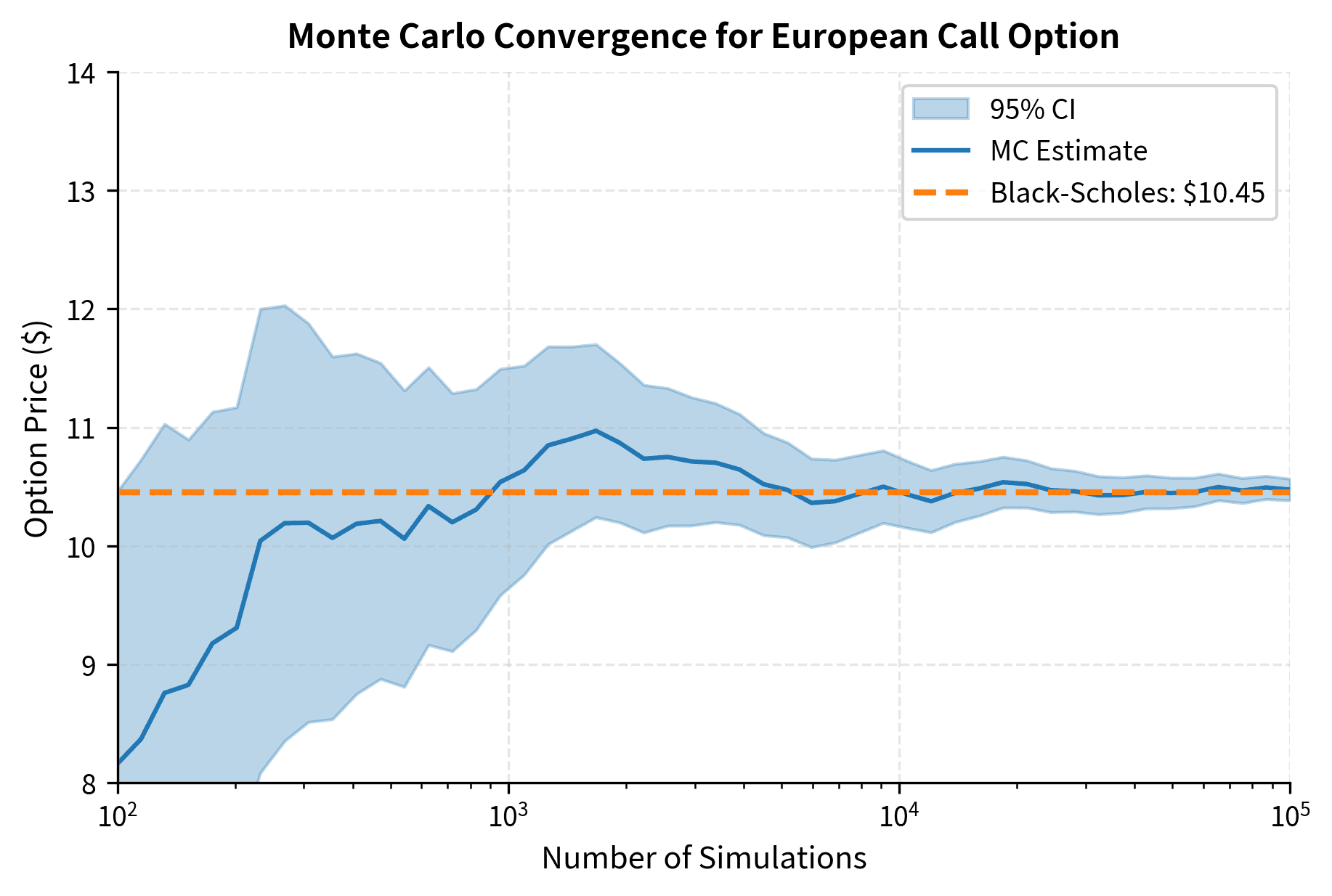
Monte Carlo converges at rate , so quadrupling simulations halves the error. While slower than analytical methods when available, Monte Carlo handles complex payoffs and path-dependent options where no closed-form solution exists.
Limitations and Practical Considerations
The framework of calculus and differential equations has important limitations in financial applications.
Model Risk
Differential equations describe idealized dynamics. Financial systems exhibit regime changes, jumps, and structural breaks that smooth differential equations cannot capture. The 2008 financial crisis revealed models that performed well in normal conditions but failed catastrophically when market dynamics shifted. Solutions to differential equations represent model outputs, not market reality. Continuous compounding, for instance, assumes interest is credited infinitely often, which approximates but never equals actual bank practices.
Numerical Precision
Numerical integration introduces approximation errors that compound in complex calculations. Option pricing often involves nested integrations. Expected values over terminal distributions may depend on path integrals. Small errors can magnify, particularly for deep out-of-the-money options or long-dated instruments. Production systems require careful attention to numerical stability, convergence criteria, and error estimation. Calling scipy.integrate.quad appears simple but uses sophisticated adaptive algorithms that can still fail for ill-behaved functions.
Computational Tractability
Some problems are analytically solvable but computationally expensive. Others have no closed-form solution at all. The trade-off between analytical solutions and numerical methods depends on the application.
- Real-time pricing demands fast analytical formulas
- Risk management may accept slower Monte Carlo for complex instruments
- Research often explores both approaches to validate results
Understanding which tools apply when, and their computational costs, is as important as the mathematics itself.
Summary
This chapter developed integral calculus and differential equations as tools for quantitative finance. The key concepts and their financial applications include:
Integral Calculus:
- The definite integral computes accumulated quantities, including total returns, present values of cash flow streams, and expected payoffs
- The Fundamental Theorem of Calculus connects integration to antiderivatives, enabling analytical solutions when antiderivatives exist
- Integration techniques (substitution, parts) appear throughout derivative pricing and risk calculations
Continuous Compounding:
- The limit of discrete compounding leads to the continuous formula
- This formula arises as the solution to the differential equation
- Time-varying rates require integrating along the yield curve:
Differential Equations:
- First-order linear ODEs model portfolio growth, mean-reverting rates, and asset depreciation
- Separation of variables solves many fundamental financial models
- Logistic equations capture bounded growth in market adoption and saturation
- Numerical methods (like
scipy.integrate.odeint) handle equations without closed-form solutions
Connection to Advanced Topics:
- The Black-Scholes PDE extends ODE concepts to option pricing
- Stochastic differential equations add randomness to the deterministic models studied here
- Present value calculations under risk-neutral measures are expectations computed via integration
These foundations enable the continuous-time finance models used in modern quantitative practice. The next chapters will build on these tools, introducing probability distributions and stochastic processes that capture the randomness inherent in financial markets.
Key Parameters
The key parameters for integral calculus and differential equations in finance are:
- r: Interest rate or discount rate. Appears in continuous compounding and determines how future cash flows are discounted to present value.
- T: Time horizon or maturity. Longer time periods amplify the effects of compounding and discounting.
- κ (kappa): Mean reversion speed in models like Vasicek. Higher values mean faster reversion to the long-term mean, with half-life .
- θ (theta): Long-term mean in mean-reverting models. The equilibrium level toward which the process gravitates.
- δ (delta): Depreciation or decay rate. Determines how quickly asset values decline, with half-life .
- K: Carrying capacity in logistic growth models. The maximum sustainable value that bounds growth.
- μ (mu): Drift rate in growth models. Represents the expected rate of return or growth per unit time.
- σ (sigma): Volatility parameter. Measures the magnitude of random fluctuations in stochastic models.
Quiz
Ready to test your understanding? Take this quick quiz to reinforce what you've learned about integral calculus and differential equations in finance.

Comments