

Master derivatives, gradients, and optimization techniques essential for quantitative finance. Learn Greeks, portfolio optimization, and Lagrange multipliers.
Choose your expertise level to adjust how many terms are explained. Beginners see more tooltips, experts see fewer to maintain reading flow. Hover over underlined terms for instant definitions.
Differential Calculus and Optimization Basics
Quantitative finance is fundamentally about measuring change and finding optimal solutions. When a trader asks "how much will my option's value change if the stock moves by one dollar?" they are asking a calculus question. When a portfolio manager asks "what asset allocation maximizes my risk-adjusted return?" they are posing an optimization problem. Differential calculus describes rates of change, while optimization theory helps us find the best outcomes under given constraints.
These two branches of mathematics form an inseparable partnership in finance: the ability to measure rates of change allows us to understand sensitivities, which in turn allows us to identify when we have reached an optimal point. The gradient of a function tells us how fast things are changing and in which direction we should move to improve our position. This interplay between measurement and improvement lies at the heart of quantitative decision-making.
This chapter builds the calculus foundation you will use throughout this book. We begin with derivatives as measures of sensitivity, then extend to functions of multiple variables using partial derivatives and gradients. From there, we develop the machinery for finding optimal solutions, both unconstrained and constrained, ending with the Lagrange multiplier technique used in modern portfolio theory. Finally, we examine convexity, a property that guarantees the optima we find are truly the best solutions possible.
Derivatives and Rates of Change
The derivative of a function measures its instantaneous rate of change. If represents a quantity that depends on , then the derivative tells us how rapidly changes as changes. In finance, this sensitivity analysis is essential. We constantly need to understand how outputs respond to changes in inputs.
To understand derivatives, consider what it means to measure change. If you know the value of your portfolio today and knew its value yesterday, you can compute how much it changed over that day. But that average change over a day may obscure important dynamics that occurred during trading hours. The derivative captures what happens as we shrink the time interval to an infinitesimally small moment, revealing the true instantaneous rate of change at any point in time.
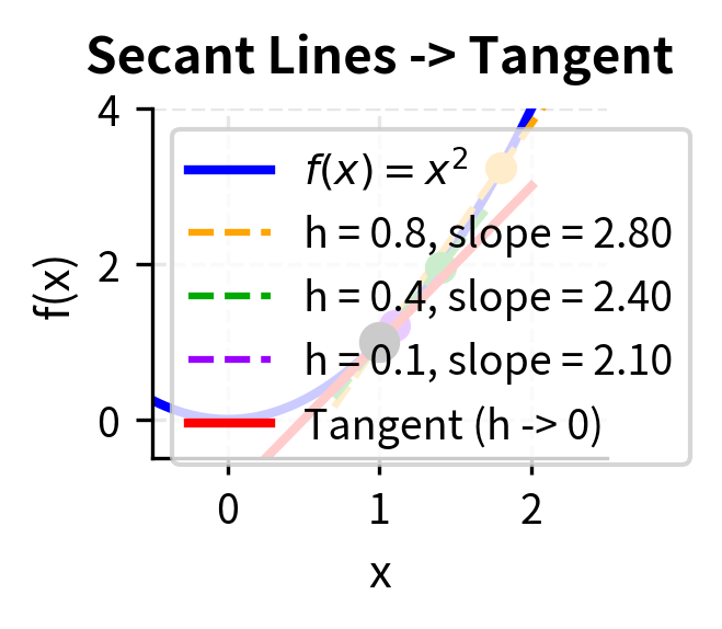
The formal definition of the derivative captures this limiting process precisely. We start by computing the average rate of change over an interval of size , then we ask what happens to this average as becomes vanishingly small. When this limit exists and is well-defined, we have successfully captured the instantaneous rate of change.
The derivative of a function at a point is defined as the limit of the difference quotient:
where:
- : the function value at point
- : a small increment approaching zero
- : the change in function value over the interval
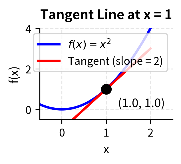
When this limit exists, we say is differentiable at . The derivative represents the slope of the tangent line to the function at that point.
The geometric interpretation of the derivative illuminates its meaning. If you graph the function and zoom in on any differentiable point, the curve begins to look more and more like a straight line. The derivative gives the slope of this line, the tangent line that best approximates the function at that point. This slope tells us the direction and steepness of the function's change. A positive derivative means the function is increasing; a negative derivative means it is decreasing; and a zero derivative indicates a momentary pause, a point where the function is neither rising nor falling, which often signals a maximum or minimum.
Financial Interpretation of Derivatives
In finance, derivatives (the calculus concept, not the financial instruments) appear everywhere as sensitivity measures. Consider a simple example: the profit function of a market maker.
The relationship between the mathematical concept of a derivative and financial instruments called "derivatives" is no coincidence. Financial derivatives like options and futures derive their value from underlying assets, and understanding how that value changes requires calculating mathematical derivatives. The sensitivity of an option's price to the underlying stock price is literally the derivative of the option pricing function with respect to the stock price.
Suppose a market maker's daily profit depends on trading volume :
where:
- : daily profit in dollars
- : trading volume in units
- : revenue from bid-ask spread ($0.001 per unit)
- : fixed daily operating costs
- : market impact costs that grow quadratically with volume
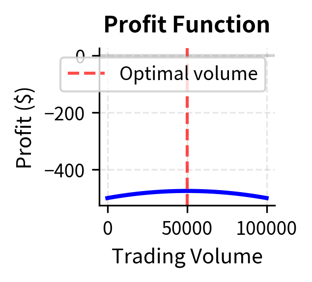
This profit function captures three fundamental aspects of market making. The first term represents the revenue the market maker earns from the bid-ask spread: every time a unit is traded, the market maker captures a small spread of $0.001. If this were the only factor, profit would grow linearly forever. The constant term of 500 represents the fixed costs that must be paid regardless of volume: technology, salaries, rent, and regulatory fees. These costs must be covered before any profit is realized.
The quadratic term is the most financially interesting. It represents market impact costs that grow with the square of volume. This non-linear relationship arises because as a market maker trades more, they begin to move the market against themselves. Large orders require taking increasingly unfavorable prices, and the cumulative effect of these adverse price movements grows more than proportionally with volume. This is why the coefficient is negative and multiplies .
The first term represents revenue (a small spread earned per unit volume), the constant represents fixed costs, and the quadratic term captures market impact costs that grow with volume. The derivative:
where:
- : the marginal profit at volume level
- : the marginal revenue per unit (the bid-ask spread)
- : the marginal market impact cost, which increases linearly with volume
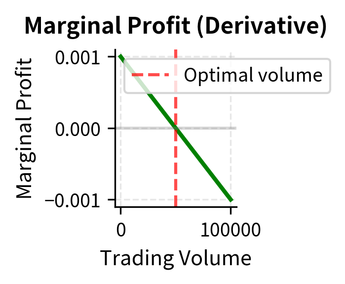
This is the marginal profit, meaning the additional profit from one more unit of trading volume. When , increasing volume increases profit. When , the market impact costs outweigh the spread revenue.
Notice how the derivative transforms our understanding of the profit function. The original function tells us total profit at any volume level, but the derivative tells us whether we should increase or decrease our volume from the current level. This marginal perspective is precisely what an economist or trader needs for decision-making. We don't ask "what is our profit?" but rather "should we trade more or less?" The derivative answers this second, more actionable question.
At 50,000 units, the marginal profit is zero, indicating we have found the profit-maximizing volume. Beyond this point, each additional unit of volume actually reduces total profit due to market impact.
The zero marginal profit condition is not a coincidence but a fundamental principle. At the optimal volume, the marginal revenue from one more trade (the bid-ask spread of $0.001) exactly equals the marginal market impact cost. Any volume below this point leaves money on the table: the spread earned exceeds the impact cost, so trading more increases profit. Any volume above this point destroys value: the impact cost exceeds the spread earned. This balance condition, where marginal benefit equals marginal cost, recurs throughout economics and finance as the defining characteristic of optimal decisions.
Option Sensitivities: The Greeks
The most famous application of derivatives in finance is the calculation of option sensitivities, known as "the Greeks." These measure how an option's price responds to changes in various inputs.
The Greeks earned their collective name because most of them are denoted by Greek letters, following a tradition from early options theory. Each Greek captures one dimension of risk, and together they form a complete local picture of how an option's value will change as market conditions evolve. Understanding the Greeks is essential for anyone who trades or hedges options, because they translate mathematical sensitivities into dollar amounts.
Consider a European call option with price that depends on the underlying stock price , time to expiration , volatility , and risk-free rate . Each Greek is a partial derivative of with respect to one of these inputs:
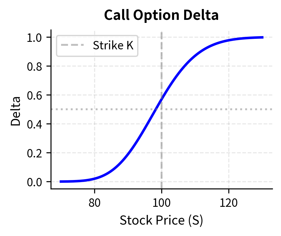
- Delta (): measures sensitivity to stock price changes
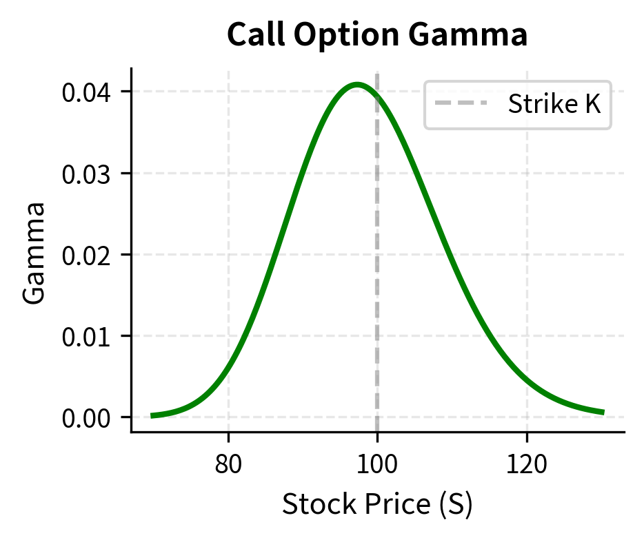
- Gamma (): measures the rate of change of delta
- Theta (): measures sensitivity to time decay
- Vega (): measures sensitivity to volatility changes
- Rho (): measures sensitivity to interest rate changes
where:
- : the call option price
- : the current stock price
- : time to expiration
- : implied volatility of the underlying
- : risk-free interest rate
Delta is the most frequently used Greek in practice. If an option has a delta of 0.5, this means that for every $1 increase in the stock price, the option price increases by approximately $0.50. Traders use delta to determine how many shares of stock they need to hold to hedge their option positions. A portfolio that is "delta neutral" has offsetting sensitivities: the options move up when the stock moves down, and vice versa, resulting in little net change in portfolio value for small stock movements.
Gamma adds depth to the delta picture by measuring how delta itself changes. An option with high gamma has a delta that changes rapidly as the stock price moves. This is particularly important near expiration for at-the-money options, where gamma can spike dramatically. A trader who is long gamma benefits from large moves in either direction, while a trader who is short gamma is exposed to the risk that their delta hedge becomes stale quickly.
The Greeks provide a complete local picture of option sensitivity. Delta and Gamma capture price risk; Theta captures time decay; Vega captures volatility risk; and Rho captures interest rate risk. Together, they enable traders to understand and hedge their exposures across all major risk dimensions.
We will derive these explicitly when we cover the Black-Scholes model in a later chapter. For now, understand that each Greek answers a practical question: "If this input changes by a small amount, how much does my option position change in value?"
Multivariable Calculus
Financial models rarely depend on a single variable. A portfolio's return depends on the returns of all constituent assets. An option's value depends on price, time, volatility, and interest rates simultaneously. This requires extending calculus to functions of multiple variables.
The transition from single-variable to multivariable calculus is conceptually straightforward and practically important. In single-variable calculus, we had one direction of change. In multivariable calculus, we have infinitely many directions we could move. Understanding how the function changes in each of these directions requires new mathematical machinery.
Partial Derivatives
When a function depends on multiple variables, the partial derivative measures the rate of change with respect to one variable while holding all others constant.
The key conceptual insight is that partial derivatives treat other variables as if they were constants. If you want to know how portfolio return changes when you adjust the weight in one particular asset, you imagine all other weights frozen in place and observe how the return responds to that single change. This "one variable at a time" approach simplifies the analysis but also limits what we can learn. The true behavior of the function involves simultaneous changes in multiple variables, which we will address with gradients and directional derivatives.
For a function , the partial derivative with respect to is:
where:
- : the variable with respect to which we differentiate
- : a small increment approaching zero
- : all other variables, held constant during differentiation
We treat all variables except as constants and differentiate normally.
The notation uses the curly "partial" symbol ∂ rather than the regular "d" used in single-variable calculus. This notational distinction serves as a reminder that we are holding other variables fixed. The computation itself follows the same rules as ordinary differentiation: we simply treat the other variables as constants and differentiate with respect to the variable of interest.
Consider a simple two-asset portfolio where total return depends on the returns and of each asset and their weights and :
The partial derivatives tell us how sensitive total return is to each input:
The first equation says that the sensitivity of portfolio return to the first weight equals the return of that asset. The second says that sensitivity to the first asset's return equals its weight in the portfolio. Both are intuitive, but partial derivatives make this reasoning precise.
These results have immediate practical interpretations. The partial derivative with respect to weight tells a portfolio manager: "If you increase the allocation to asset 1 by 1%, and that asset has a return of 10%, your portfolio return increases by 0.10 percentage points." The partial derivative with respect to return tells a risk manager: "If asset 1's return changes by 1%, and you hold 40% in that asset, your portfolio return changes by 0.4 percentage points." These linear sensitivities form the foundation of risk factor models used throughout the industry.
The Gradient Vector
Collecting all partial derivatives of a function into a single vector gives us the gradient, a fundamental object in optimization.
The gradient represents the multivariable generalization of the derivative. While a single-variable derivative tells us the rate of change in the only direction available, the gradient in multiple dimensions tells us how to combine changes in each direction to achieve the maximum rate of increase. This makes the gradient more than a collection of sensitivities; it is a directional guide pointing toward improvement.
The gradient of a function is the vector of all partial derivatives:
where:
- : the gradient operator (nabla) applied to , producing a vector
- : the partial derivative of with respect to the -th variable
- : the dimension of the input space
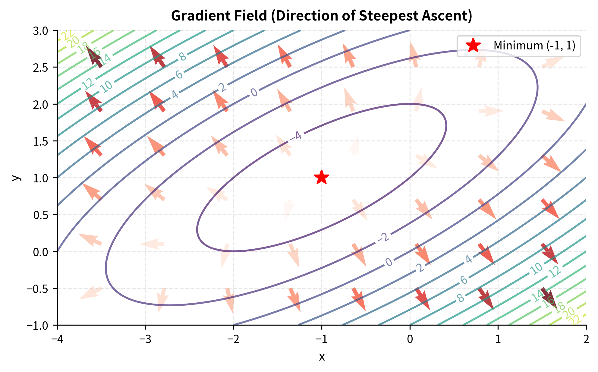
The gradient points in the direction of steepest ascent of the function.
The gradient's direction is crucial: at any point, the gradient points toward the direction in which increases most rapidly. Its magnitude indicates how steep that increase is. This property makes the gradient the workhorse of optimization algorithms, as we will see shortly.
To understand why the gradient points in the direction of steepest ascent, consider the directional derivative, which measures the rate of change of in any specified direction. Analysis shows that this rate of change is maximized when we move in the same direction as the gradient. Conversely, moving opposite to the gradient gives the steepest descent, which is precisely what we want when minimizing a function.
The magnitude of the gradient, computed as , tells us how rapidly the function is changing in the steepest direction. A large gradient magnitude indicates a region where the function is changing rapidly; a small magnitude indicates a relatively flat region. When the gradient magnitude is exactly zero, we have reached a critical point where the function has no preferred direction of change, which typically indicates a local minimum, maximum, or saddle point.
The gradient at (1, 2) is [2, 0], meaning the function increases most rapidly in the positive direction at that point, with no change in the direction. This tells us that from (1, 2), moving in the positive direction increases the function value, while moving in the positive direction has no first-order effect.
The fact that the -component of the gradient is zero at this point reveals that we are on a "ridge" or "valley" in the -direction. The function is neither increasing nor decreasing as we vary while holding fixed at 1. This doesn't mean we're at the optimum; it just means we're at a stationary point with respect to at this particular -value. To find the true minimum, we need to find a point where both components of the gradient are zero simultaneously.
Numerical Differentiation
While analytical derivatives are preferred when available, we often need to compute derivatives numerically, especially for complex models or when working with black-box functions.
In many practical situations, we have access to a function only through evaluations. We can plug in values and observe outputs, but we don't have a closed-form expression that allows symbolic differentiation. This occurs frequently when dealing with simulation-based models, legacy software systems, or complex financial instruments where the pricing function involves numerous nested calculations. Numerical differentiation provides a way to approximate derivatives using only function evaluations.
The simplest approach uses the finite difference approximation:
However, the central difference formula provides better accuracy:
where:
- : the derivative we are approximating
- : a small step size (often around to for central differences in double precision, depending on scaling)
- and : function evaluations at points symmetric around
The central difference achieves accuracy compared to for the forward difference, because the symmetric evaluation cancels first-order error terms. In practice, choosing involves a trade-off: too large introduces truncation error, too small introduces floating-point rounding error.
The error analysis behind these approximations reveals why the central difference is superior. When we Taylor expand and around , the first-order terms appear with the same sign in both expansions but are subtracted in the central difference formula. The second-order terms appear with the same sign and cancel when we take the difference. This cancellation is what improves the accuracy from to . The forward difference lacks this symmetry and retains larger error terms.
The choice of step size represents a fundamental tension in numerical computation. A smaller reduces truncation error because we're better approximating the limit as . But computers store numbers with finite precision, and when becomes too small, the difference involves subtracting nearly equal numbers, which amplifies rounding errors. The optimal balances these effects and often falls around to for central differences in double-precision floating-point numbers, depending on scaling.
The numerical gradient matches the analytical result to within floating-point precision, validating our implementation. This technique becomes invaluable when analytical derivatives are unavailable or too complex to derive by hand.
Unconstrained Optimization
Optimization is the process of finding the best solution among all feasible alternatives. In unconstrained optimization, we seek to minimize or maximize a function without restrictions on the input variables.
The goal of optimization is to find the point or points where a function achieves its best value. "Best" might mean smallest (for costs and risks) or largest (for returns and profits). In unconstrained optimization, we are free to choose any values for the input variables; there are no boundaries or restrictions to respect. While this may seem simpler than constrained optimization, the principles we develop here form the foundation for handling constraints as well.
First-Order Conditions
The first step in finding an optimum is identifying critical points, where the gradient equals zero.
The intuition behind the first-order condition is compelling. At a point where the function achieves a maximum or minimum, you cannot improve by moving in any direction. If the gradient were nonzero, it would point toward a direction of ascent, meaning you could increase the function by moving that way. At a minimum, there's no direction of descent available; at a maximum, there's no direction of ascent. The only way both can fail to exist is if the gradient is the zero vector.
If has a local minimum or maximum at an interior point , and is differentiable at , then:
Points satisfying this condition are called critical points or stationary points.
It is essential to understand that the first-order condition is necessary but not sufficient for an optimum. A zero gradient tells us we have found a critical point, but not all critical points are minima or maxima. Some are saddle points, where the function increases in certain directions and decreases in others. Think of a mountain pass: it is a minimum when you traverse the pass but a maximum when you go perpendicular to it. Both directions through this critical point have zero derivative, yet the point is neither a global maximum nor a global minimum.
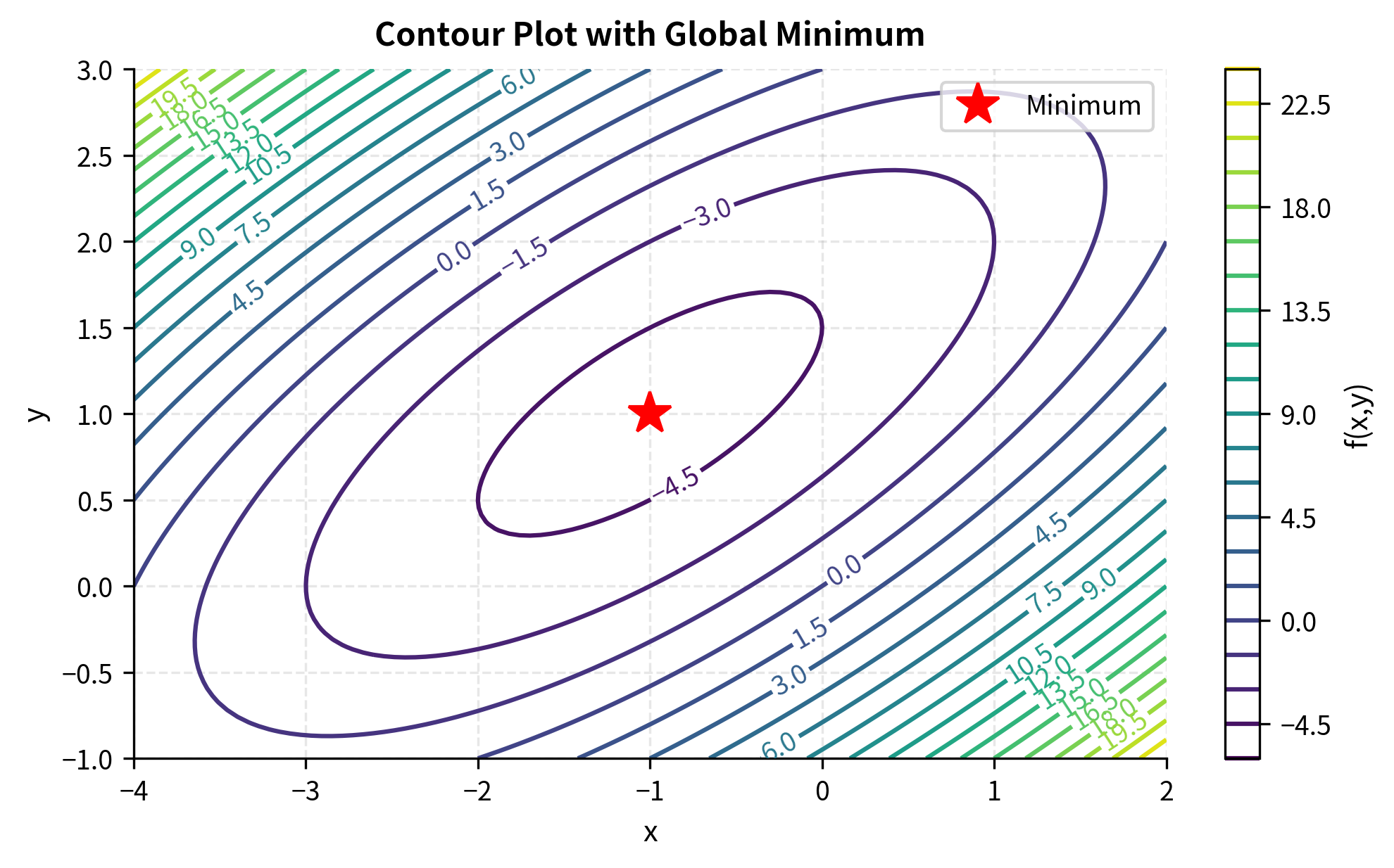
Setting the gradient to zero gives us a system of equations. For our earlier quadratic function:
Solving this system:
The critical point is at (-1, 1), where the gradient is indeed zero.
Second-Order Conditions and the Hessian
A zero gradient tells us we have found a critical point, but not whether it is a minimum, maximum, or saddle point. To classify critical points, we need second-order information encoded in the Hessian matrix.
The Hessian matrix extends the concept of the second derivative to multiple dimensions. Just as the second derivative of a single-variable function tells us about the function's curvature (whether it curves upward or downward), the Hessian tells us about curvature in all directions simultaneously. Because there are infinitely many directions in multidimensional space, this information is naturally organized into a matrix rather than a single number.
The Hessian matrix of a function is the matrix of second partial derivatives:
For functions with continuous second derivatives, the Hessian is symmetric.
The diagonal entries of the Hessian capture the pure second derivatives: how the rate of change with respect to one variable itself changes as that variable varies. The off-diagonal entries capture the mixed partial derivatives: how the rate of change with respect to one variable changes as another variable varies. The symmetry of the Hessian, known as the equality of mixed partials or Clairaut's theorem, holds for functions with continuous second derivatives and reflects the fundamental fact that the order of differentiation doesn't matter for such functions.
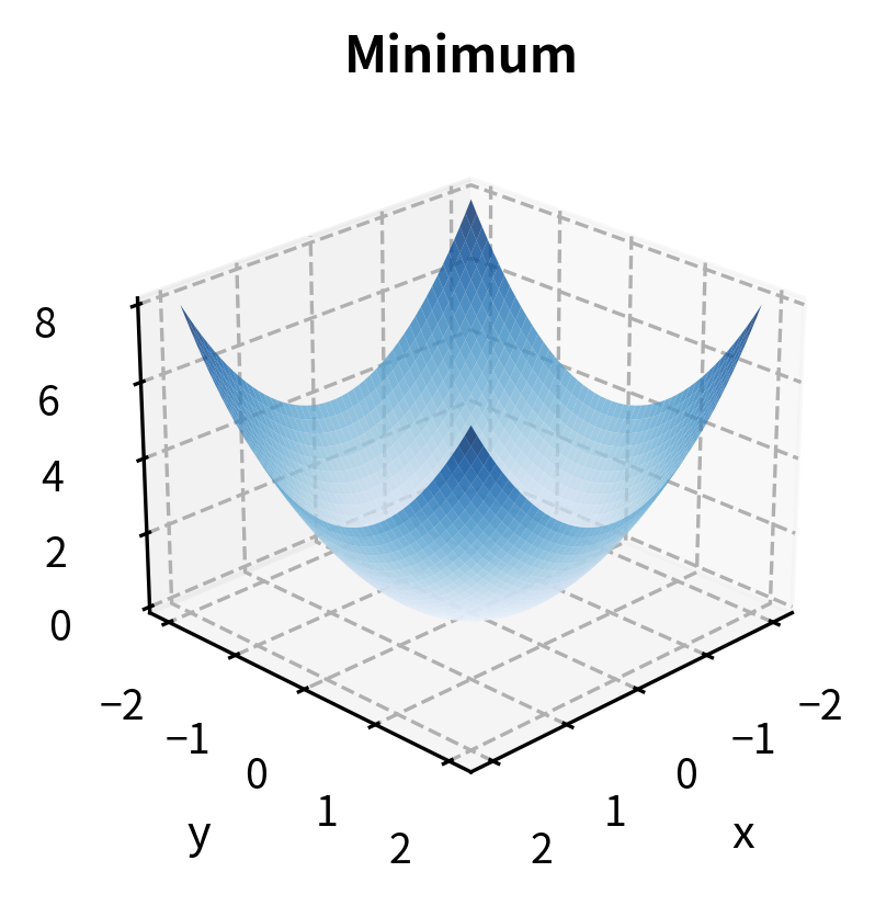
The eigenvalues of the Hessian at a critical point determine its nature:
- All eigenvalues positive: local minimum
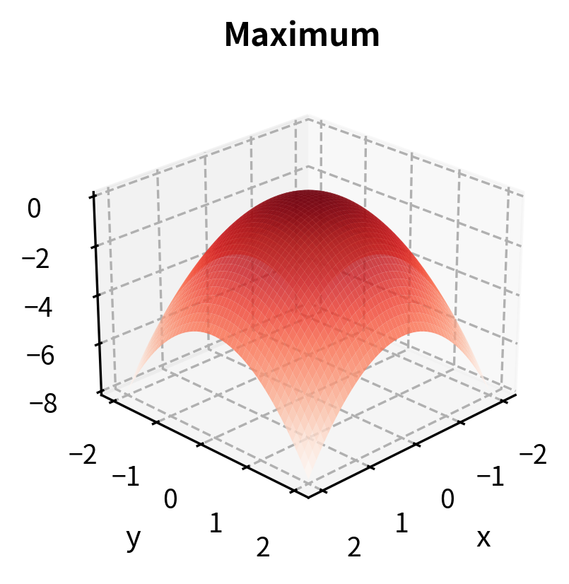
- All eigenvalues negative: local maximum
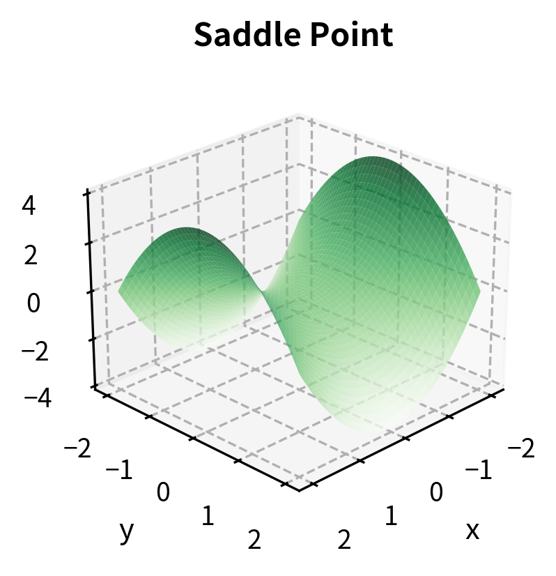
- Mixed signs: saddle point
The connection between eigenvalues and the nature of critical points comes from a deep result in linear algebra. The eigenvalues of the Hessian represent the curvatures of the function along the principal directions (the eigenvectors). If all these curvatures are positive, the function curves upward in every direction, creating a bowl shape characteristic of a minimum. If all are negative, it curves downward in every direction, creating an inverted bowl characteristic of a maximum. Mixed signs create the saddle shape, curving up in some directions and down in others.
For our quadratic function, the Hessian is constant:
Both eigenvalues are positive, confirming that the critical point (-1, 1) is a local minimum. Since the function is quadratic with a positive definite Hessian, this minimum is also global.
The fact that the Hessian is constant for this function is a special property of quadratic functions. The second derivatives of a quadratic function are constants because taking two derivatives of a quadratic term yields a constant. This constancy means the curvature is the same everywhere, which simplifies both analysis and computation. For more general functions, the Hessian varies from point to point, and we must evaluate it specifically at the critical point to determine the point's nature.
Gradient Descent
Gradient descent is the most fundamental optimization algorithm in machine learning and quantitative finance. Since the gradient points uphill, we find a minimum by repeatedly stepping in the opposite direction.
Gradient descent is conceptually straightforward. At any point, we compute the gradient to determine the direction of steepest ascent, then move in the opposite direction to descend toward lower values. By repeating this process, we trace out a path that, under appropriate conditions, leads to a minimum. This iterative approach is particularly valuable for high-dimensional problems where analytical solutions are impossible or impractical.
The update rule is:
where:
- : the current iterate at step
- : the next iterate after the update
- : the learning rate (step size), controlling how far we move in each iteration
- : the gradient evaluated at the current point, indicating the direction of steepest ascent
The negative sign is crucial: we subtract the gradient because we want to descend, not ascend. The learning rate scales the step size, determining how far we move in the descent direction. This single parameter has an outsized influence on the algorithm's behavior.
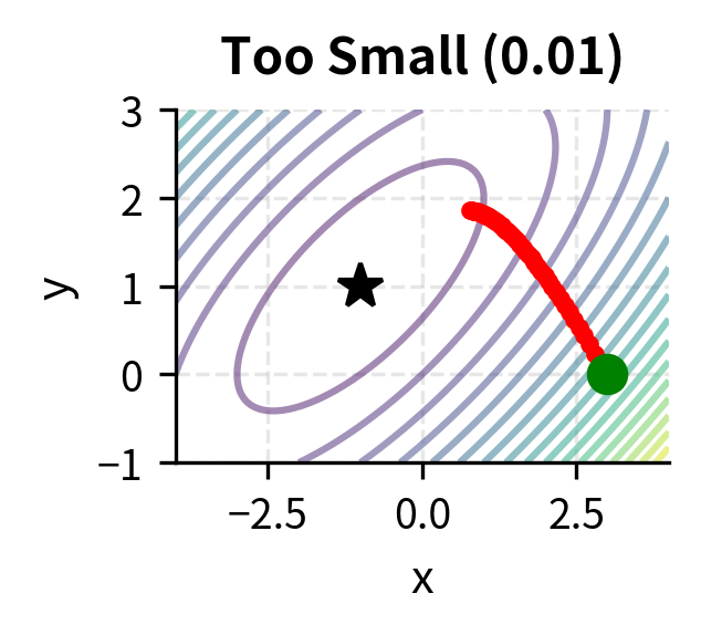
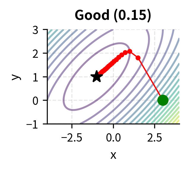
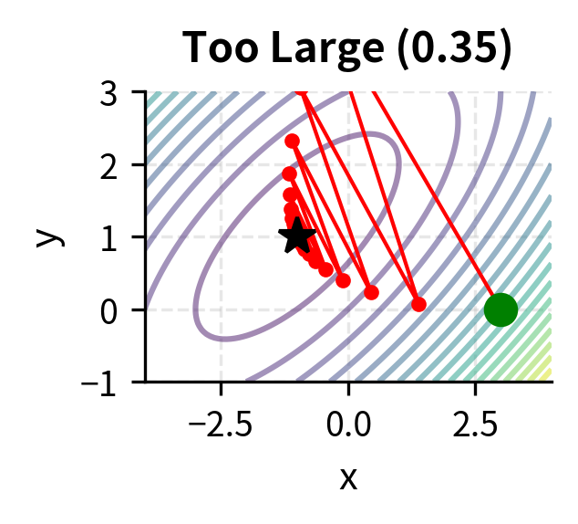
Choosing is crucial. If it is too large, the algorithm may overshoot and diverge. If it is too small, convergence becomes painfully slow.
The learning rate embodies a fundamental trade-off in optimization. A large learning rate allows rapid progress when far from the minimum, but risks overshooting when close. Imagine trying to land on a narrow valley floor: large steps might cause you to bounce from one side to the other, never settling down. A small learning rate ensures stable progress but may require many iterations to reach the minimum, particularly in flat regions where the gradient is small. Advanced variants of gradient descent, such as momentum methods and adaptive learning rates, address these issues by adjusting the step size dynamically.
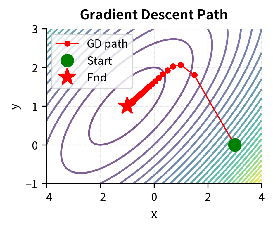
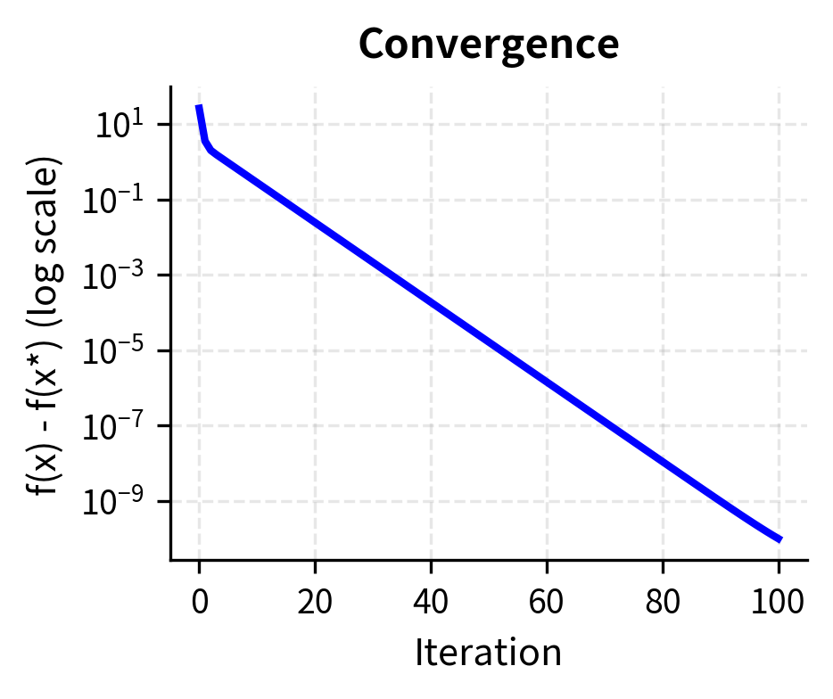
The algorithm converges to the true minimum in relatively few iterations. The convergence plot shows the characteristic linear convergence rate of gradient descent on smooth strongly convex functions.
Constrained Optimization and Lagrange Multipliers
Many financial optimization problems involve constraints. A portfolio manager cannot invest more than 100% of capital. A risk manager must ensure volatility stays below a threshold. A trader faces position limits. These constraints lead to constrained optimization problems.
Constraints reflect the realities of financial markets and institutions. Regulations prohibit certain positions. Risk limits prevent excessive concentration. Budget constraints ensure we don't spend money we don't have. Constrained optimization finds the best achievable outcome while respecting these limitations. This typically means finding the solution that would be optimal if we could stretch the constraints slightly.
The Lagrangian Method
The method of Lagrange multipliers handles equality constraints by converting a constrained problem into an unconstrained one. Consider minimizing subject to the constraint .
Lagrange's approach embeds the constraint into the objective function. Rather than treating optimization and constraint satisfaction as separate tasks, we create a new function, the Lagrangian, that penalizes constraint violations. Finding the stationary points of this Lagrangian simultaneously solves for the optimal point and ensures the constraint is satisfied.
The Lagrangian combines the objective function and constraints:
where:
- : the Lagrangian function
- : the decision variables we are optimizing
- : the Lagrange multiplier, measuring the sensitivity of the optimum to the constraint
- : the objective function we want to minimize or maximize
- : the equality constraint that must be satisfied
At a constrained optimum, the gradient of the Lagrangian with respect to all variables (including ) equals zero.
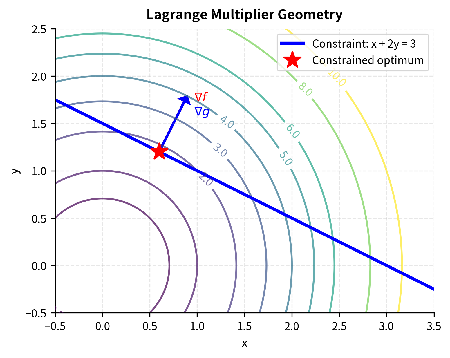
The key insight is geometric. At a constrained optimum, the gradient of the objective function must be parallel to the gradient of the constraint function. If they were not parallel, you could move along the constraint surface in a direction that decreases the objective.
To understand this geometric insight more deeply, imagine standing on a hill (the objective function) while constrained to walk along a path (the constraint surface). At the optimal point along this path, the steepest uphill direction on the original surface points directly toward or away from the path itself; there is no component along the path. If there were such a component, you could walk along the path in that direction and climb higher on the hill, contradicting the optimality of your current position. This perpendicularity between the gradient and the constraint surface is precisely what the Lagrange conditions capture.
Mathematically, this means:
Combined with the constraint , these equations form a system we can solve for both the optimal point and the multiplier .
The system of equations consists of equations in unknowns: equations from setting the gradient of the Lagrangian with respect to equal to zero, and one equation from the constraint . This matches the number of unknowns, which are the components of and the single multiplier . When the equations are independent, we can solve for a unique solution, giving us both the optimal point and the shadow price.
Worked Example: Portfolio Allocation
Consider allocating between two assets to minimize portfolio variance, subject to achieving a target expected return.
This problem encapsulates the fundamental challenge of portfolio management: balancing risk against return. Investors want high returns, but higher expected returns typically require accepting more risk. The minimum-variance portfolio for a given target return represents the most efficient way to achieve that return, using diversification to squeeze out unnecessary risk.
Let and be the weights in assets 1 and 2, with expected returns and , variances and , and correlation . The portfolio variance is:
where:
- : portfolio variance
- : portfolio weights for assets 1 and 2
- : variances of assets 1 and 2
- : correlation between the two assets
- : covariance contribution from the interaction between assets
This variance formula reveals the mathematics of diversification. The first two terms represent the variance contributions from each asset individually, scaled by the square of their weights. The third term captures the interaction between assets through their covariance. When correlation is less than 1, this interaction term is smaller than it would be for perfectly correlated assets, allowing the portfolio variance to be less than the weighted average of individual variances. This reduction is the diversification benefit.
We want to minimize subject to:
- Target return:
- Full investment:
The Lagrangian is:
where:
- : Lagrange multiplier for the return constraint, representing the marginal variance cost of achieving additional return
- : Lagrange multiplier for the budget constraint, representing the shadow price of capital
The two constraints serve different purposes. The return constraint ensures we achieve our investment objective; its multiplier tells us how much additional variance we must accept per unit of additional expected return. The budget constraint ensures we are fully invested, neither leveraged nor holding cash; its multiplier represents the value of an additional dollar of capital to invest.
The optimizer found that to achieve an 8% return with minimum variance, we should put 60% in the higher-return, higher-risk asset and 40% in the lower-return, lower-risk asset. This balances the return target against risk minimization.
Interpreting Lagrange Multipliers
The Lagrange multiplier has a powerful economic interpretation: it measures the shadow price of the constraint, or how much the optimal objective value would change if we relaxed the constraint slightly.
Shadow prices connect abstract optimization theory to concrete economic decisions. When a constraint binds (meaning it is satisfied with equality), its shadow price tells us the marginal value of relaxing that constraint. If the shadow price is high, we would benefit significantly from loosening the constraint; if it's low, the constraint is not particularly costly. This information is crucial for managers deciding where to focus efforts on expanding capacity or negotiating constraint modifications.
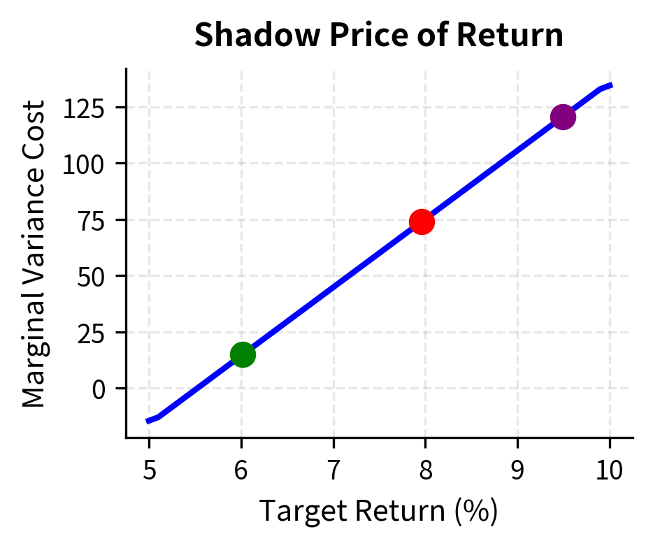
For our portfolio problem, the multiplier on the return constraint tells us how much additional variance we would need to accept to achieve a slightly higher target return. This is the marginal cost of return in units of variance.
In practical terms, if the Lagrange multiplier for the return constraint equals 0.02, this means that pushing our target return from 8% to 8.1% (an increase of 0.1 percentage points) would increase the minimum achievable variance by approximately , or equivalently increase the standard deviation by a calculable amount. Portfolio managers use this information to decide whether incremental return targets justify the additional risk.
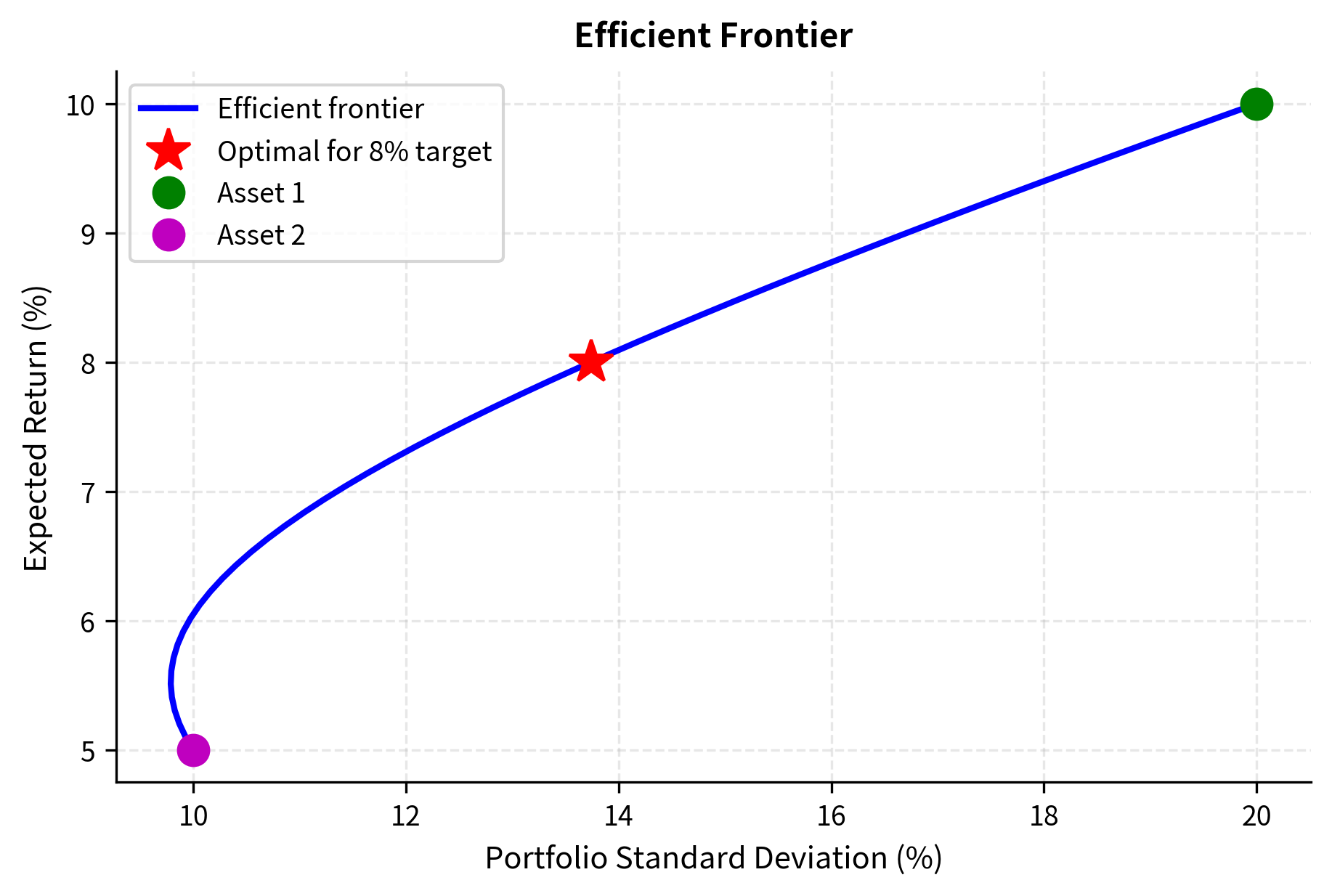
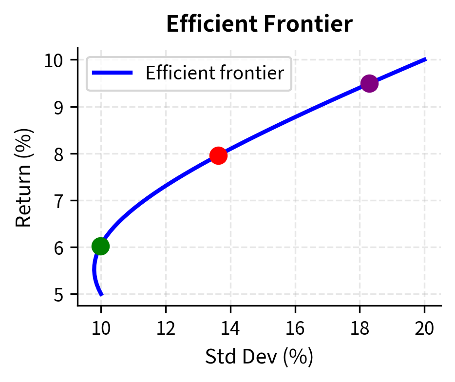
The efficient frontier shows the fundamental risk-return trade-off. Every point on this curve represents the minimum possible risk for a given return target. The Lagrange multiplier on the return constraint measures how the minimum achievable variance changes when we increase the return requirement.
Convexity
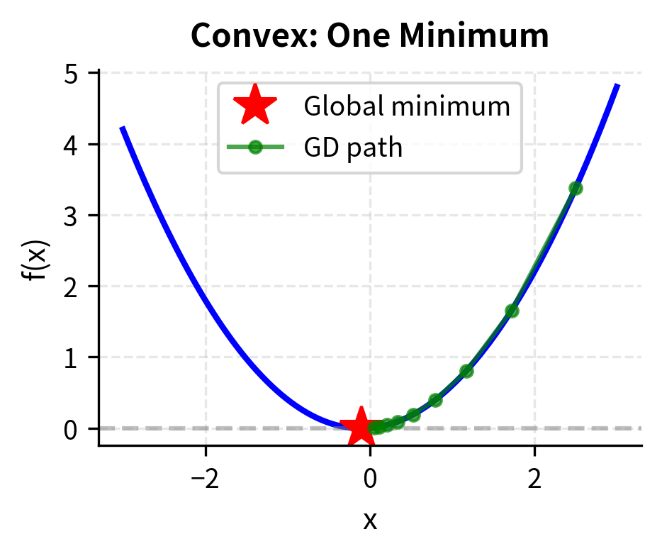
Convexity is a key structural property in optimization. When a function is convex, any local minimum is automatically a global minimum, dramatically simplifying the search for optimal solutions.
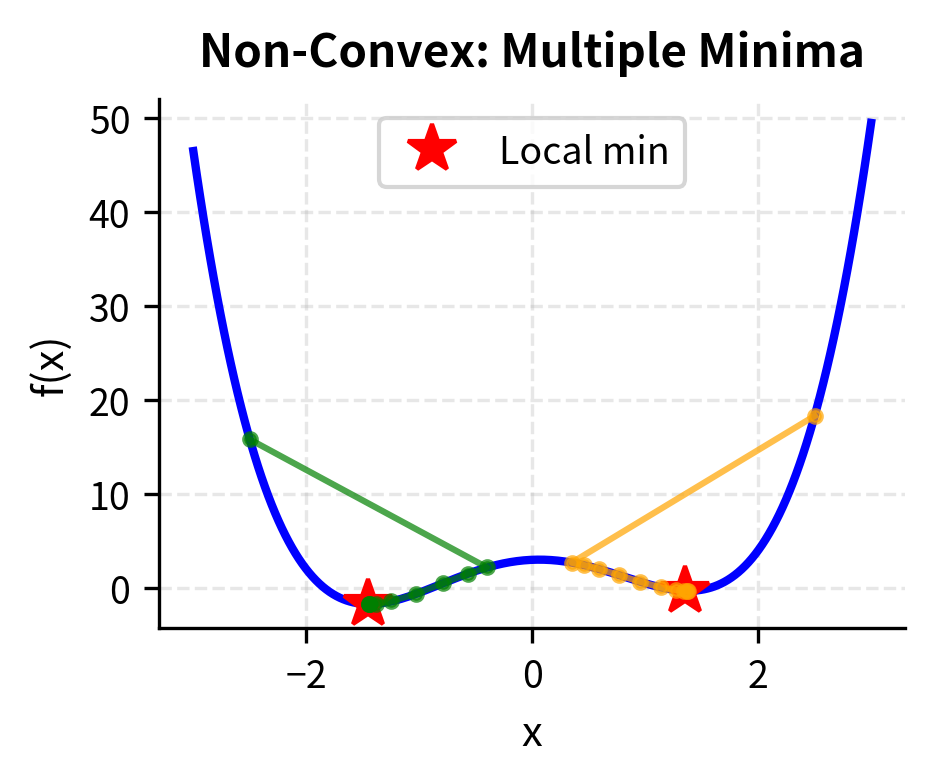
Convexity provides essential guarantees in optimization. In non-convex optimization, we face a landscape with potentially many valleys. Gradient-based methods can get stuck in any of them with no guarantee of finding the deepest one. In convex optimization, there is a single global valley (sometimes with a flat bottom), and any local minimum you reach is globally optimal. This qualitative difference transforms optimization from a computationally hard problem into a tractable one.
Definition and Intuition
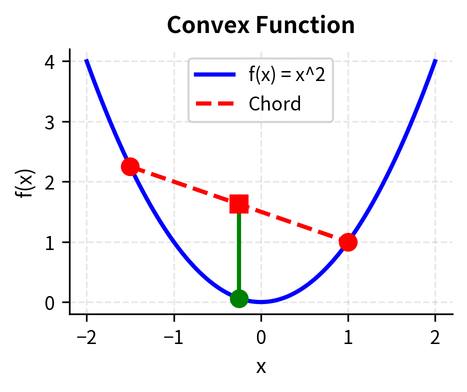
The formal definition of convexity captures a simple geometric idea. A function is convex if the line segment connecting any two points on its graph lies above the graph itself. Alternatively, if you interpolate between two input points and evaluate the function at the interpolated point, you get a value no larger than if you had interpolated between the function values at the original points.
A function is convex if for any two points and and any :
where:
- : any two points in the domain of
- : a convex combination weight (interpolation parameter)
- : a point on the line segment between and
- : the corresponding point on the chord connecting and
Geometrically, this means the line segment connecting any two points on the graph lies above the graph itself.
The definition says that interpolating between any two points in the domain and evaluating the function gives a value at most as large as interpolating between the function values at those points. Intuitively, a convex function "curves upward" everywhere.
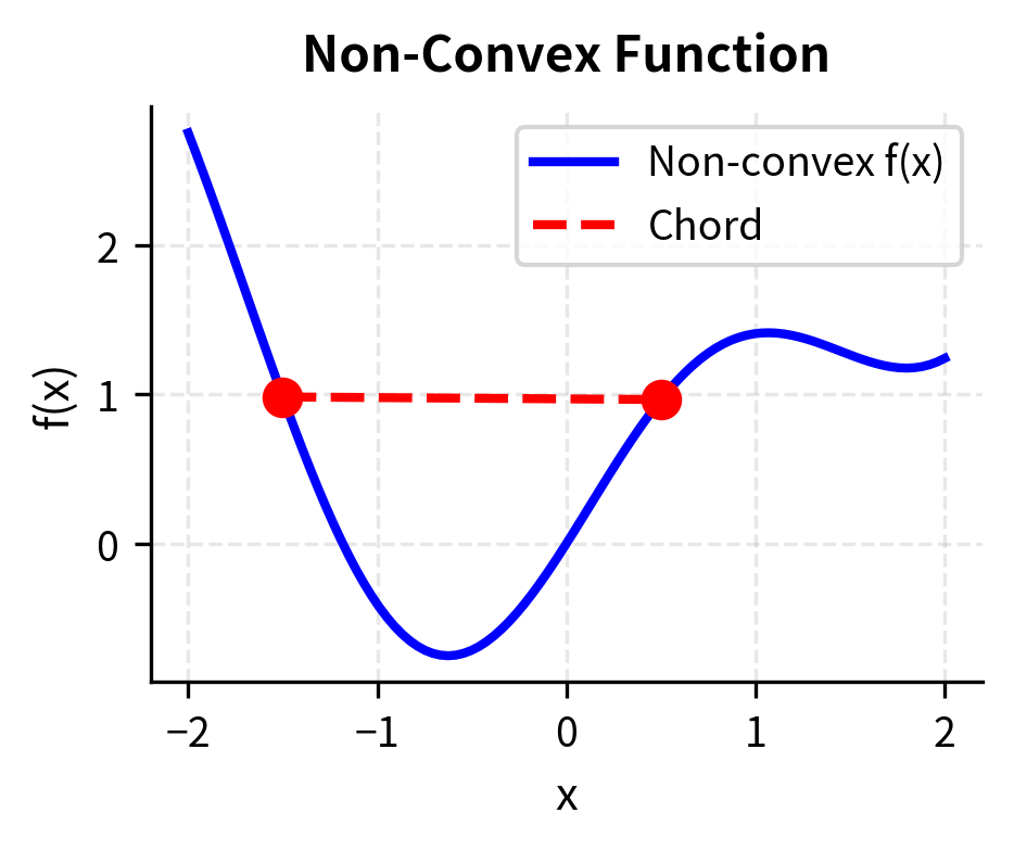
Consider a bowl placed on a table. If you pick any two points on the rim of the bowl and stretch a string between them, the string remains above or on the surface of the bowl everywhere along its length. This is the defining characteristic of convexity. A non-convex surface might dip below such a string, creating regions where the surface rises above the interpolated line.
The parameter can be thought of as a "mixing" proportion. When , we are entirely at point ; when , we are entirely at point ; and intermediate values of give us intermediate points along the segment. The convexity inequality states that the function value at any such intermediate point is at most the correspondingly weighted average of the function values at the endpoints.
Testing for Convexity
For twice-differentiable functions, convexity can be checked using the Hessian matrix.
A function is convex if and only if its Hessian is positive semidefinite everywhere. All eigenvalues of must be non-negative.
The function is strictly convex if is positive definite everywhere (all eigenvalues ).
The intuition behind this condition connects to the function's curvature. The Hessian captures how the gradient changes as we move through the space. Positive semidefiniteness means that in every direction, the function curves upward (or is flat), never downward. This ensures that following the gradient downhill always leads to the global minimum, with no "valleys" that could trap us at suboptimal points.
To understand why the Hessian condition characterizes convexity, recall that the Hessian appears in the second-order Taylor expansion of the function. Around any point , the function behaves approximately as a quadratic: . The quadratic term determines the local curvature. For a positive semidefinite , this term is always non-negative, meaning the function curves upward or remains flat in every direction. This local property, holding everywhere, implies global convexity.
For our quadratic portfolio variance function:
where is the covariance matrix. The Hessian of this function is:
Since covariance matrices are positive semidefinite by construction (variances of portfolios cannot be negative), the portfolio variance function is convex. This guarantees that the minimum-variance portfolio we found is the global minimum.
This result is not merely mathematically elegant but practically significant. When we solve for the minimum-variance portfolio, we know we have found the truly optimal solution, not just a locally optimal one. There are no hidden better solutions lurking elsewhere in the feasible region. This guarantee of global optimality provides confidence in the solution and justifies the widespread use of mean-variance optimization in portfolio management.
Why Convexity Matters in Finance
Convexity has significant practical implications in quantitative finance:
Portfolio optimization is convex. The mean-variance optimization problem involves minimizing a convex function (portfolio variance) subject to linear constraints. This means any local optimum found by a standard optimization algorithm is globally optimal. There are no local minima traps to worry about.
This convexity is why Markowitz's mean-variance framework remains practical after sixty years. Portfolio managers can confidently compute optimal portfolios knowing that numerical algorithms will find the true optimum. Without convexity, the same problem would require searching an exponentially large space of potential local minima, making reliable optimization infeasible for large portfolios.
Risk measures should be convex. A convex risk measure ensures that diversification never increases risk. Variance and standard deviation are convex; Value-at-Risk is not convex in general. This aligns with the financial intuition that spreading investments reduces risk.
The convexity of risk measures formalizes the diversification principle. If is a convex risk measure and we combine two portfolios and with weights and , then . The risk of the combined portfolio is at most the weighted average of the individual risks, and typically strictly less. This inequality is precisely what makes diversification valuable: combining positions reduces overall risk.
Non-convexity creates computational challenges. When objective functions are non-convex, optimization becomes much harder. Multiple local minima may exist. Gradient-based methods can get stuck. Problems involving integer constraints (such as selecting a discrete number of assets) or certain complex risk measures lose the convexity guarantee, requiring more sophisticated solution techniques.
Non-convex problems arise frequently in practice despite the convenience of convex formulations. Transaction costs with fixed components (minimum fees regardless of trade size) introduce non-convexity. Cardinality constraints (hold at most 30 stocks) are inherently non-convex. Some risk measures like Value-at-Risk under certain distributions violate convexity. When facing such problems, practitioners must either accept potentially suboptimal solutions from local search methods or employ computationally expensive global optimization techniques.
Practical Implementation with SciPy
SciPy's optimize module provides robust implementations of optimization algorithms suitable for most financial applications.
Different optimization algorithms have different strengths. BFGS (a quasi-Newton method) typically converges quickly for smooth problems by approximating the Hessian. Nelder-Mead is derivative-free and robust but slower. The choice depends on problem characteristics, including smoothness, dimension, availability of gradients, and computational budget.
Handling Bounds and Constraints
Real financial problems often involve bounds (no short selling: ) and multiple constraints (budget, sector limits, etc.).
The optimizer allocates across all three assets to achieve the 9% target return with minimum variance, respecting the no-short-selling constraint.
Key Parameters
The key parameters for portfolio optimization are:
- μ (mu): Expected returns vector. Higher expected returns for an asset increase its optimal allocation, all else equal.
- Σ (Sigma): Covariance matrix capturing asset variances and correlations. Lower correlations enable greater diversification benefits.
- Target return: The required portfolio return, which determines the position on the efficient frontier.
- Bounds: Constraints on individual weights (e.g., no short selling requires w ≥ 0).
- Learning rate (α): For gradient descent, controls step size. Too large causes divergence; too small slows convergence.
Limitations and Practical Considerations
While calculus and optimization are useful tools for quantitative finance, practitioners should know their limitations.
Model sensitivity. Optimization results can be highly sensitive to input parameters. In portfolio optimization, small changes in expected returns or covariances can produce dramatically different optimal allocations. This phenomenon (called estimation error amplification) means that optimizers may act as "error maximizers" when inputs are estimated with uncertainty. Techniques like shrinkage estimation, robust optimization, and resampling can help mitigate this sensitivity.
Local vs. global optima. While convex problems guarantee global optimality, many real-world problems are non-convex. Factor timing strategies, options with complex payoffs, and problems with transaction costs often exhibit multiple local minima. For these problems, gradient descent may converge to suboptimal solutions depending on initialization. Global optimization methods like simulated annealing, genetic algorithms, or multi-start approaches become necessary, at the cost of increased computational burden.
Numerical precision. Finite precision arithmetic can cause issues in optimization, especially near singular or ill-conditioned matrices. Covariance matrices estimated from returns can become nearly singular when the number of assets approaches the number of observations. Regularization techniques and careful numerical implementations help maintain stability.
Constraints in practice. Real trading constraints are often more complex than simple equality or inequality constraints. Transaction costs create path-dependence. Integer constraints (minimum lot sizes) make problems combinatorially hard. Regulatory constraints may involve complex interactions between positions. These practical complexities often require specialized algorithms beyond standard calculus-based optimization.
Despite these limitations, the framework in this chapter remains the foundation for portfolio management, derivatives pricing, and risk management. Understanding derivatives as sensitivities, gradients as optimization directions, and convexity as a guarantee of optimality provides essential intuition that extends to more advanced techniques.
Summary
This chapter established the calculus and optimization foundations for quantitative finance:
Derivatives as sensitivities: The derivative measures how a function changes in response to its inputs. In finance, derivatives quantify sensitivities. Marginal profit, option Greeks, and portfolio risk exposures all rely on this fundamental concept.
Multivariable calculus: Partial derivatives extend this to functions of many variables, measuring sensitivity to each input individually. The gradient vector collects these sensitivities and points toward steepest ascent.
Unconstrained optimization: Critical points occur where the gradient vanishes. The Hessian matrix of second derivatives determines whether these points are minima, maxima, or saddle points. Gradient descent provides an iterative algorithm for finding minima.
Constrained optimization: Lagrange multipliers transform constrained problems into unconstrained ones by incorporating constraints into the objective. The multipliers have economic interpretations as shadow prices that measure the marginal cost of binding constraints.
Convexity: A convex function has no local minima traps, so any critical point is a global minimum. Portfolio variance is convex, ensuring mean-variance optimization has a globally optimal solution. Testing for convexity via the Hessian's eigenvalues determines whether this guarantee applies.
These tools appear throughout quantitative finance. The next chapters will apply them to probability and statistics, where we optimize likelihood functions to estimate parameters, and to portfolio theory, where mean-variance optimization produces the efficient frontier.
Quiz
Ready to test your understanding? Take this quick quiz to reinforce what you've learned about differential calculus and optimization in quantitative finance.

Comments