

Learn how DeepMind's Chinchilla scaling laws revolutionized LLM training by proving models should use 20 tokens per parameter for compute-optimal performance.

This article is part of the free-to-read Language AI Handbook
Choose your expertise level to adjust how many terms are explained. Beginners see more tooltips, experts see fewer to maintain reading flow. Hover over underlined terms for instant definitions.
Chinchilla Scaling Laws
In March 2022, a paper from DeepMind titled "Training Compute-Optimal Large Language Models" upended conventional wisdom about how to train large language models. The paper introduced Chinchilla, a 70 billion parameter model that outperformed the 280 billion parameter Gopher despite using the same computational budget. This result challenged the prevailing approach of building ever-larger models and revealed that the field had been systematically undertraining its models on data.
As we discussed in the Kaplan Scaling Laws chapter, the original OpenAI scaling work suggested that model size should increase faster than dataset size as compute budgets grow. This led labs to prioritize larger models, sometimes training them on relatively small amounts of data. Chinchilla demonstrated that this approach was suboptimal, showing that model size and training tokens should scale together in roughly equal proportion.
The DeepMind Experiments
The Chinchilla paper is notable for its careful methods. Rather than relying on a single experimental approach, the DeepMind team used three independent methods to estimate optimal scaling, finding very consistent results across all three. This agreement between different approaches gives us strong confidence in the conclusions. When three different methods of measuring the same phenomenon all point to the same answer, we can trust that answer far more than if it came from a single experiment. We examine each approach in detail to understand both the methodology and the insights each reveals.
Approach 1: Fixing Model Sizes
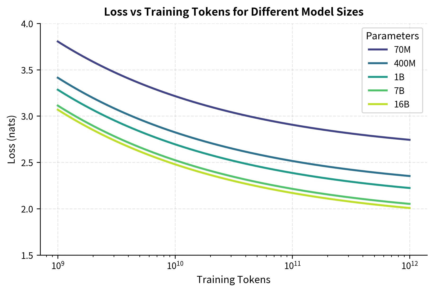
The first approach trained over 400 models ranging from 70 million to 16 billion parameters. For each model size, the team varied the number of training tokens and measured the resulting loss. This produced loss curves as a function of training tokens for each model size.
The intuition behind this approach is straightforward: if we hold model size constant and simply vary how much data we train on, we can see exactly how each model size benefits from additional training. Some models might saturate quickly, suggesting they've learned all they can from the available data. Others might continue improving steadily, indicating they could benefit from even more training. By mapping these curves across many model sizes, we build a comprehensive picture of how different architectures respond to different data quantities.
From these curves, the team extracted the minimum loss achievable at each compute budget. Here compute for parameters and training tokens, and the factor of 6 accounts for both forward and backward passes across all operations. By examining which model size achieved the lowest loss at each compute level, they could determine the optimal allocation between parameters and data.
The key insight from this approach was that for any fixed compute budget, there exists an optimal model size, and training either too large or too small a model results in worse performance. Models that were too large couldn't be trained on enough data given the compute constraint, while models that were too small couldn't capture sufficient complexity regardless of training duration. This finding shows a key trade-off in neural network training: we must balance the model's capacity to represent complex patterns against its opportunity to learn those patterns from data. Neither capacity nor data alone determines performance. Their interaction does.
Approach 2: IsoFLOP Curves
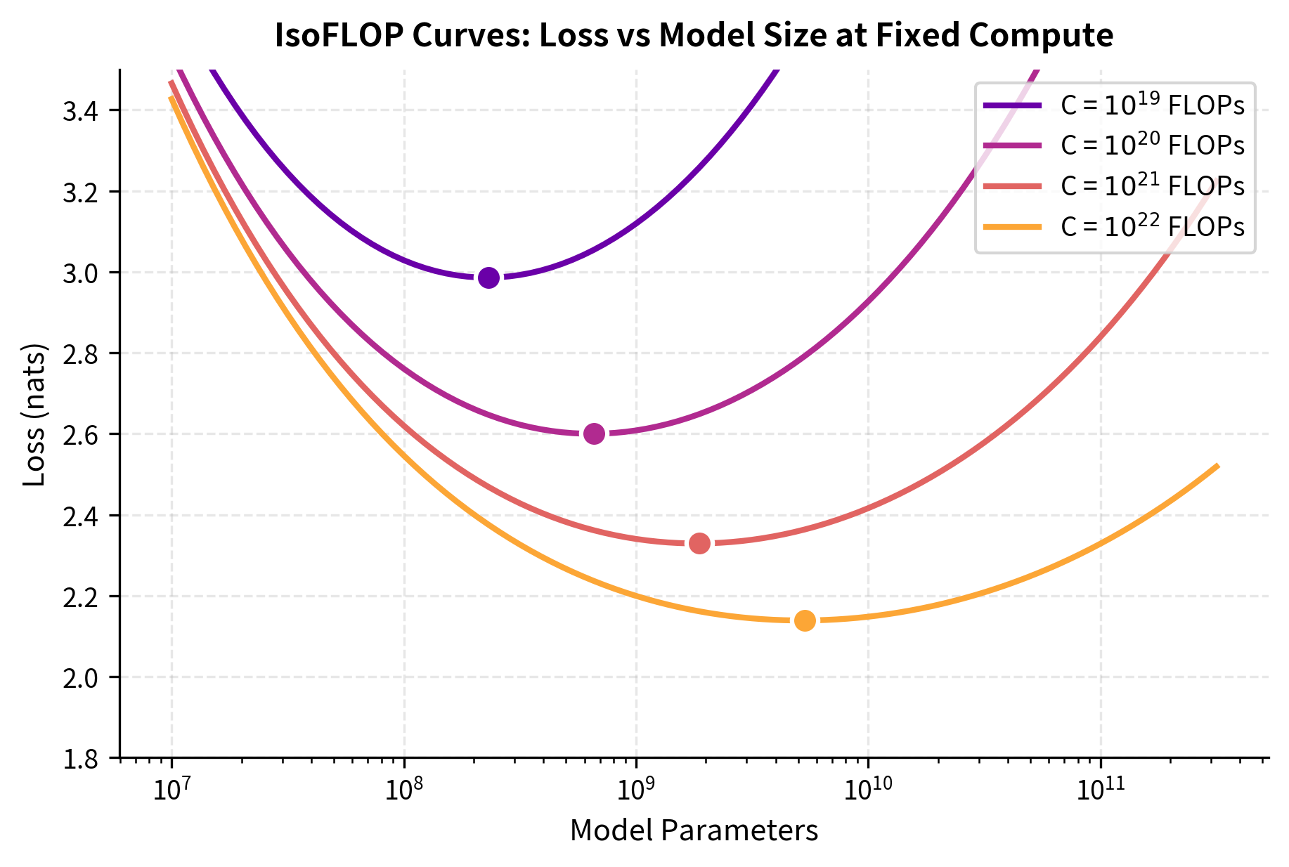
The second approach defined several fixed compute budgets (measured in FLOPs) and trained many models at each budget. For a given compute budget , the team explored different allocations: some configurations used more parameters with fewer training tokens, while others used fewer parameters with more training tokens.
This approach inverts the question from the first method: rather than asking "how does performance vary as we give a fixed model more data?", it asks "given a fixed computational budget, how should we divide that budget between model capacity and training duration?" This framing directly addresses the practical question for any team with a finite compute budget: should we build a bigger model and train it less, or build a smaller model and train it more?
This created "iso-FLOP" curves showing how loss varies with model size at fixed compute. Each curve exhibited a clear minimum corresponding to the compute-optimal allocation. As the compute budget increased, this optimal point shifted to larger models, but importantly, the optimal dataset size grew at a similar rate. The shape of these curves, rising on both ends with a clear valley in the middle, visually demonstrates that extremes are costly: training a model that is too small wastes compute on redundant passes over data the model cannot fully use, while training a model that is too large wastes compute on parameters that never get enough gradient updates to learn useful representations.
Approach 3: Parametric Loss Fitting
The third approach fit a parametric function to predict loss as a function of both model size and training tokens:
where:
- : the predicted loss for a model with parameters trained on tokens
- : the number of model parameters
- : the number of training tokens
- : the irreducible entropy of natural language, the minimum loss achievable with infinite model size and infinite data
- , : learned scaling coefficients that determine how quickly loss decreases with more parameters or data
- , : learned exponents that control the rate of diminishing returns for parameters and data respectively
This functional form provides a way to understand scaling behavior. Rather than treating each data point in isolation, this approach assumes that loss follows a specific mathematical structure, then fits that structure to all observed data simultaneously. The advantage is that once we have reliable estimates of the parameters, we can extrapolate to compute regimes we haven't yet explored and predict what loss we might achieve with a model ten times larger than any we've trained.
This functional form captures three contributions to the loss:
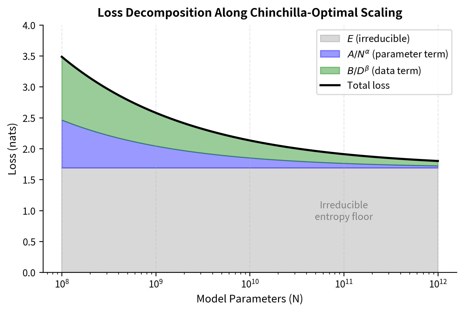
- represents the irreducible entropy of natural language, the minimum loss achievable with infinite model size and infinite data. This term sets a floor that no amount of scaling can overcome. Even a perfect model with unlimited training cannot predict language better than the inherent randomness in human text allows. This irreducible component reflects the unpredictability of language. sometimes multiple valid words could follow a given context, and no model can know which one a human will choose.
- captures how loss decreases as model capacity increases. The power law form reflects diminishing returns. Each doubling of parameters yields a fixed percentage improvement, not a fixed absolute improvement. Moving from 1 billion to 2 billion parameters provides the same relative gain as moving from 100 billion to 200 billion parameters. The exponent controls how steep this diminishing return curve is. Larger values of mean faster initial improvement but quicker saturation.
- captures how loss decreases as training data increases. Similarly, this term shows that more data helps, but with diminishing returns governed by the exponent . The first million tokens teach the model basic language structure. The next million refine that understanding. Eventually, additional tokens provide only marginal improvements as the model has already captured most learnable patterns.
By fitting this function to the experimental data, the team estimated the exponents and along with the constants , , and . These parameters then allow computation of the optimal allocation for any compute budget. This approach has predictive power: rather than running expensive experiments at every scale we care about, we can fit the function to data from smaller, cheaper experiments and then mathematically derive what should happen at larger scales.
The Chinchilla Scaling Equations
All three experimental approaches yielded consistent conclusions about optimal scaling. The Chinchilla team derived that for compute-optimal training, both model size and dataset size should scale as power laws of the compute budget:
where:
- : the optimal number of model parameters for a given compute budget
- : the optimal number of training tokens for a given compute budget
- : the total compute budget (in FLOPs)
- , : scaling exponents that determine how parameters and data should grow with compute
- The constraint follows from (compute scales with the product of parameters and tokens)
These power law relationships mean that as your compute budget grows by some factor, both the optimal model size and dataset size grow by predictable amounts determined by the exponents and . The proportionality symbol () indicates that while we don't specify the exact constants, the scaling relationship holds. If you increase compute by a factor of 100, the optimal parameter count increases by and the optimal token count increases by .
The constraint that is important because it comes from basic arithmetic rather than experiments. Since compute is approximately proportional to the product of parameters and tokens (), and since and , we have . For this equation to hold, we need . This constraint means that the exponents and cannot be chosen independently. They must sum to one, representing different ways of dividing the same computational pie.
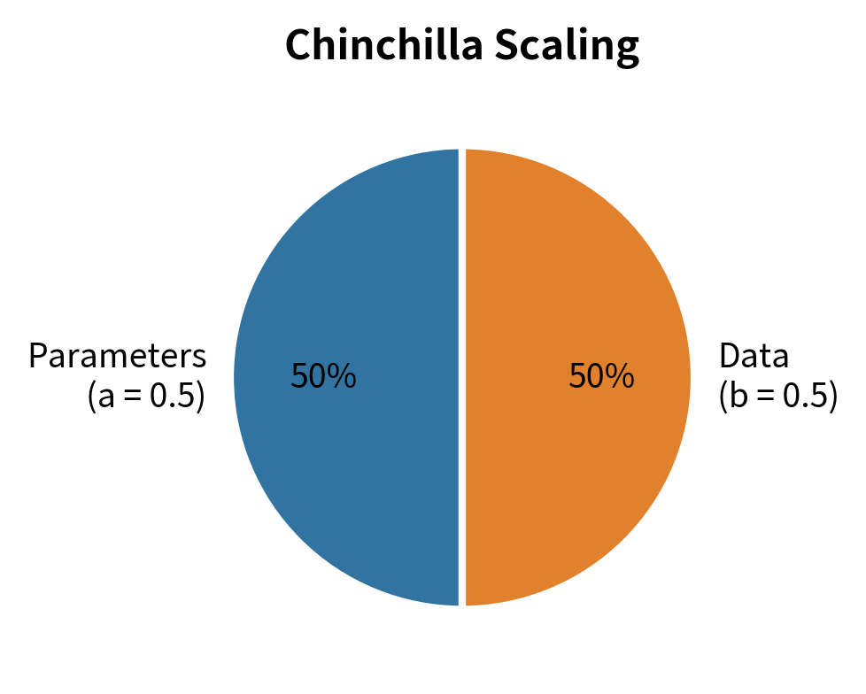
The Equal Scaling Exponents
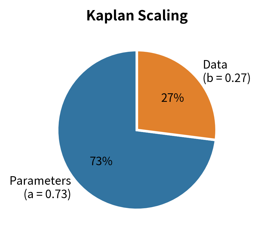
The central finding was that , meaning model size and dataset size should grow at roughly the same rate with compute. This stands in stark contrast to the Kaplan scaling laws, which suggested and , implying model size should grow much faster than dataset size.
Consider what this means in practice. With Chinchilla scaling (equal exponents around 0.5), if you increase your compute budget by a factor of 100, you should increase both your model size and your dataset size by a factor of 10 (since ). With Kaplan scaling (unequal exponents), the same 100x compute increase would suggest increasing model size by about 50x () but dataset size by only about 2x (). The difference matters: Kaplan scaling funnels most additional resources into model capacity, while Chinchilla scaling distributes resources evenly between capacity and training data.
Fitting the parametric loss model to experimental data yielded:
where:
- : the exponent governing how loss decreases with model size (from the term)
- : the exponent governing how loss decreases with training data (from the term)
These exponents determine how quickly each source of error decreases as we add parameters or data. The relatively similar values explain why balanced scaling is optimal: neither parameters nor data provide much faster diminishing returns compared to the other. If were much larger than , it would mean that increasing model size reduces loss much faster than increasing data, and we should favor parameters. If were much larger, we should favor data. But with and , both resources contribute roughly equally to loss reduction per unit of compute invested, so we should invest roughly equally in both.
Optimal Tokens Per Parameter
The most practical finding from Chinchilla is the optimal ratio of training tokens to model parameters. The analysis suggests:
where:
- : the optimal number of training tokens
- : the optimal number of model parameters
- The ratio of 20 emerges from the balanced scaling exponents ()
This means a compute-optimal model should be trained on approximately 20 tokens per parameter. A 1 billion parameter model should see roughly 20 billion tokens, a 10 billion parameter model should see 200 billion tokens, and so on.
This ratio provides a practical guideline: before training any model, you can estimate whether your training corpus is appropriately sized. Multiply your planned parameter count by 20, and that's roughly how many tokens you need for compute-optimal training. If you have fewer tokens available, you're training a model too large for your data. If you have many more tokens, you might benefit from a larger model.
This ratio is remarkably consistent across scales. The team found that deviating significantly from this ratio leads to compute inefficiency: either the model is too small to fully utilize the available training signal, or too large to be trained adequately given the data budget. The intuition is that each parameter represents a "slot" for storing learned knowledge, and 20 tokens provides enough gradient signal to fill that slot effectively. Too few tokens means the slot remains partially empty; too many tokens means the model cannot store all the patterns it could learn.
Chinchilla vs Kaplan: Understanding the Discrepancy
The Chinchilla and Kaplan scaling laws arrive at different conclusions despite both being grounded in extensive experiments. Understanding why helps clarify the details of scaling analysis.
Different Compute Ranges
The Kaplan experiments focused primarily on smaller models (up to a few hundred million parameters) with relatively limited compute budgets. The Chinchilla experiments covered a broader range, including models up to 16 billion parameters trained with significantly more compute.
Power law exponents estimated from one regime may not extrapolate to others. The Chinchilla team's larger-scale experiments revealed behavior that wasn't apparent in the smaller-scale Kaplan analysis.
Training Details Matter
The two studies used different training configurations:
| Aspect | Kaplan | Chinchilla |
|---|---|---|
| Learning rate schedule | Shorter warmup | Cosine decay with longer training |
| Number of training tokens | Fixed, relatively short | Varied extensively |
| Model architectures | GPT-style | Similar but with some modifications |
| Stopping criteria | Earlier stopping | Training to convergence |
The Kaplan analysis suggested that large models can be "early stopped" effectively, meaning you don't need to train them to convergence to achieve good performance. However, this early stopping analysis appears to have underestimated the benefits of longer training.
The Learning Rate Schedule Effect
One key difference involves learning rate scheduling. The Kaplan experiments often trained models for fewer steps than optimal, and learning rate schedules were not always tuned for the full training duration. The Chinchilla experiments used carefully tuned cosine learning rate schedules that decayed properly over the intended training length.
When you tune your learning rate schedule specifically for longer training runs, the benefit of additional training data increases. Models can extract more signal from the data because the optimization process is better matched to the training duration.
The Loss Decomposition Interpretation
Both analyses fit loss as a function of parameters and data, but with different assumptions about the functional form. The Kaplan decomposition allowed for interaction terms and considered how loss varies in suboptimal regimes differently than Chinchilla.
When fitting power laws to noisy data, small differences in the fitting procedure can lead to different exponent estimates, especially when extrapolating beyond the observed range.
Implications of Chinchilla Scaling
The Chinchilla results had immediate implications for how the field approaches language model training.
Many Models Were Undertrained
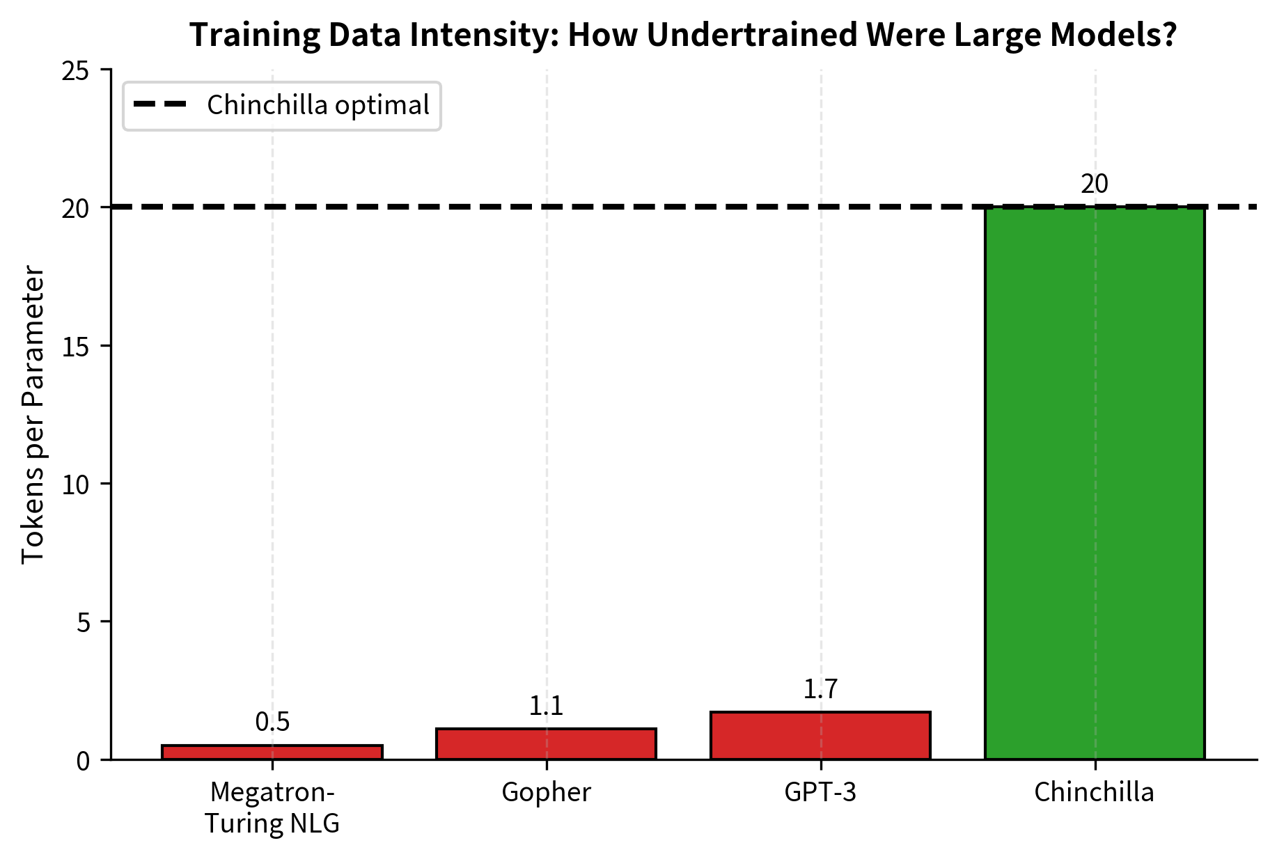
At the time of publication, most large language models had been trained well below the Chinchilla-optimal data budget:
| Model | Parameters | Training Tokens | Tokens/Parameter |
|---|---|---|---|
| GPT-3 | 175B | 300B | 1.7 |
| Gopher | 280B | 300B | 1.1 |
| Megatron-Turing NLG | 530B | 270B | 0.5 |
| Chinchilla | 70B | 1.4T | 20 |
GPT-3, despite its impressive capabilities, was trained on only 1.7 tokens per parameter, far below the Chinchilla-optimal 20 tokens. The same compute budget could have trained a smaller model to significantly better performance.
The Shift to Smaller, Better-Trained Models
Following Chinchilla, the field rapidly shifted toward training smaller models on more data. LLaMA 1 (7B to 65B parameters) trained on 1-1.4T tokens. LLaMA 2 continued this trend. The Chinchilla insight provided both economic and capability motivation: smaller models are cheaper to deploy while potentially achieving better performance than larger but undertrained alternatives.
Data Becomes the Bottleneck
If models should be trained on 20 tokens per parameter, then a 100 billion parameter model needs 2 trillion training tokens. At this scale, data availability becomes a serious constraint. High-quality text data is finite, and the Chinchilla scaling laws pushed the field toward solutions like:
- More sophisticated data filtering and deduplication
- Synthetic data generation
- Multi-epoch training on high-quality subsets
- Multimodal data incorporation
We'll explore these data-constrained scenarios in the upcoming chapter on Data-Constrained Scaling, where the Chinchilla optimum cannot be achieved due to limited data availability.
Inference Cost Considerations
The Chinchilla framing focuses purely on training compute. However, models deployed at scale accumulate inference costs that eventually dominate training costs. A smaller Chinchilla-optimal model costs less per inference request than a larger undertrained model.
This inference advantage compounds: if a 70B Chinchilla-optimal model matches the quality of a 280B undertrained model, the inference cost reduction is roughly 4x for each query. For models serving millions of requests, this adds up to large savings.
Worked Example: Computing Chinchilla-Optimal Allocations
This section shows how to compute Chinchilla-optimal model sizes and dataset sizes for a given compute budget, demonstrating how the scaling equations translate into concrete numbers.
Suppose we have a compute budget of FLOPs. Using the approximation that training FLOPs equals (where is parameters and is training tokens), and applying the Chinchilla ratio :
where:
- : the total compute budget in FLOPs
- : the number of model parameters (what we want to solve for)
- : substituting the Chinchilla-optimal token count
- The factor combines the compute constant with the optimal ratio
This substitution works because if (the Chinchilla-optimal ratio), then the compute formula simplifies to a function of alone. This constrains us to move along the Chinchilla-optimal line in the parameter-token space and determines where along that line our compute budget places us. The quadratic relationship () emerges because both and grow together. Increasing automatically increases by the same factor, so compute grows as the square.
Solving for :
where:
- : the optimal number of model parameters we're solving for
- : our target compute budget in FLOPs
- The factor 120 comes from (the compute constant 6 multiplied by the Chinchilla-optimal token ratio 20)
- The result means approximately 9 billion parameters
The square root appears because we're inverting the quadratic relationship: if , then . This means that to double our optimal model size, we need to quadruple our compute budget. Similarly, a 10x increase in compute allows only about a 3.2x increase in model size (since ).
So approximately 9 billion parameters. The optimal token count is:
where:
- : the optimal number of training tokens
- : the optimal parameter count computed above
- The factor 20 is the Chinchilla-optimal tokens-per-parameter ratio
Let's verify the compute calculation:
This verification step confirms our arithmetic and shows that the Chinchilla-optimal allocation exactly consumes the available compute budget. Nothing is wasted. Every FLOP goes toward training a model that is neither too large (which would mean insufficient training) nor too small (which would mean wasted training iterations).
For comparison, the Kaplan scaling laws would suggest allocating more to model size. Using Kaplan's and (with appropriate constants), the same compute budget would suggest roughly 30-50 billion parameters trained on only 30-50 billion tokens. The Chinchilla allocation produces better loss for the same compute because the Kaplan allocation produces a severely undertrained model. With only about 1 token per parameter, the model has insufficient opportunity to learn from data, and many of its parameters remain poorly optimized.
Code Implementation
Let's implement functions to compute Chinchilla-optimal allocations and compare them with Kaplan allocations.
Now let's compute allocations across a range of compute budgets and visualize the differences:
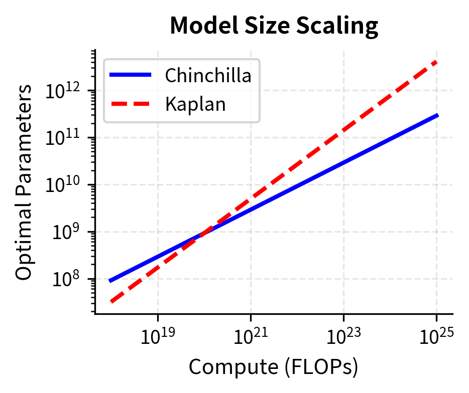
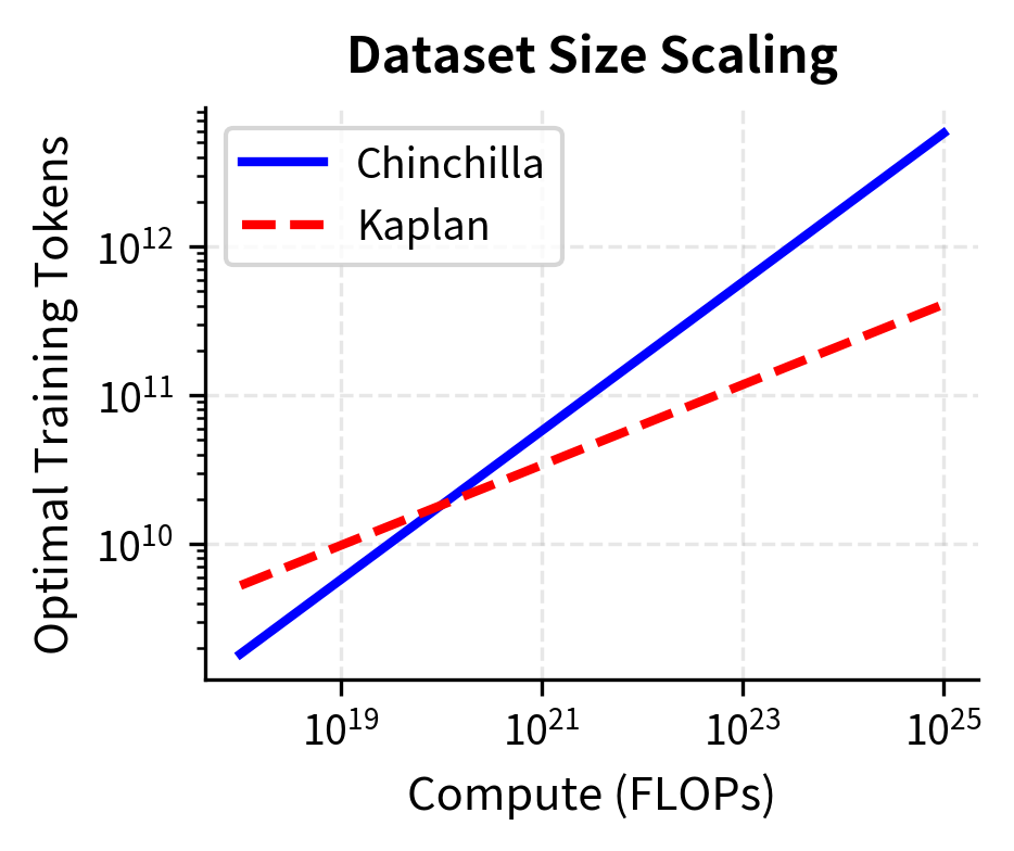
The left panel shows that as compute budgets increase, Kaplan scaling recommends much larger models than Chinchilla scaling. At FLOPs, the gap is nearly an order of magnitude. The right panel reveals the consequence: Kaplan allocates far fewer tokens to training, resulting in undertrained models. Chinchilla's balanced approach maintains the 20:1 token-to-parameter ratio across all scales.
The divergence becomes more pronounced at higher compute budgets. We can quantify this by looking at specific examples:
At FLOPs, Kaplan scaling would suggest training a model with over 20x more parameters than Chinchilla recommends, but on far fewer tokens. The Chinchilla model would likely outperform significantly because it receives adequate training data.
The comparison table reveals a clear pattern. While both methods scale up with compute, they diverge sharply in how they allocate resources. At FLOPs, Kaplan scaling recommends a 2.4T parameter model trained on only 700B tokens (0.3 tokens per parameter), while Chinchilla recommends a 91B parameter model trained on 1.8T tokens (20 tokens per parameter). The Kaplan-style allocation would produce a severely undertrained model.
Now we visualize the tokens-per-parameter ratio across compute scales:
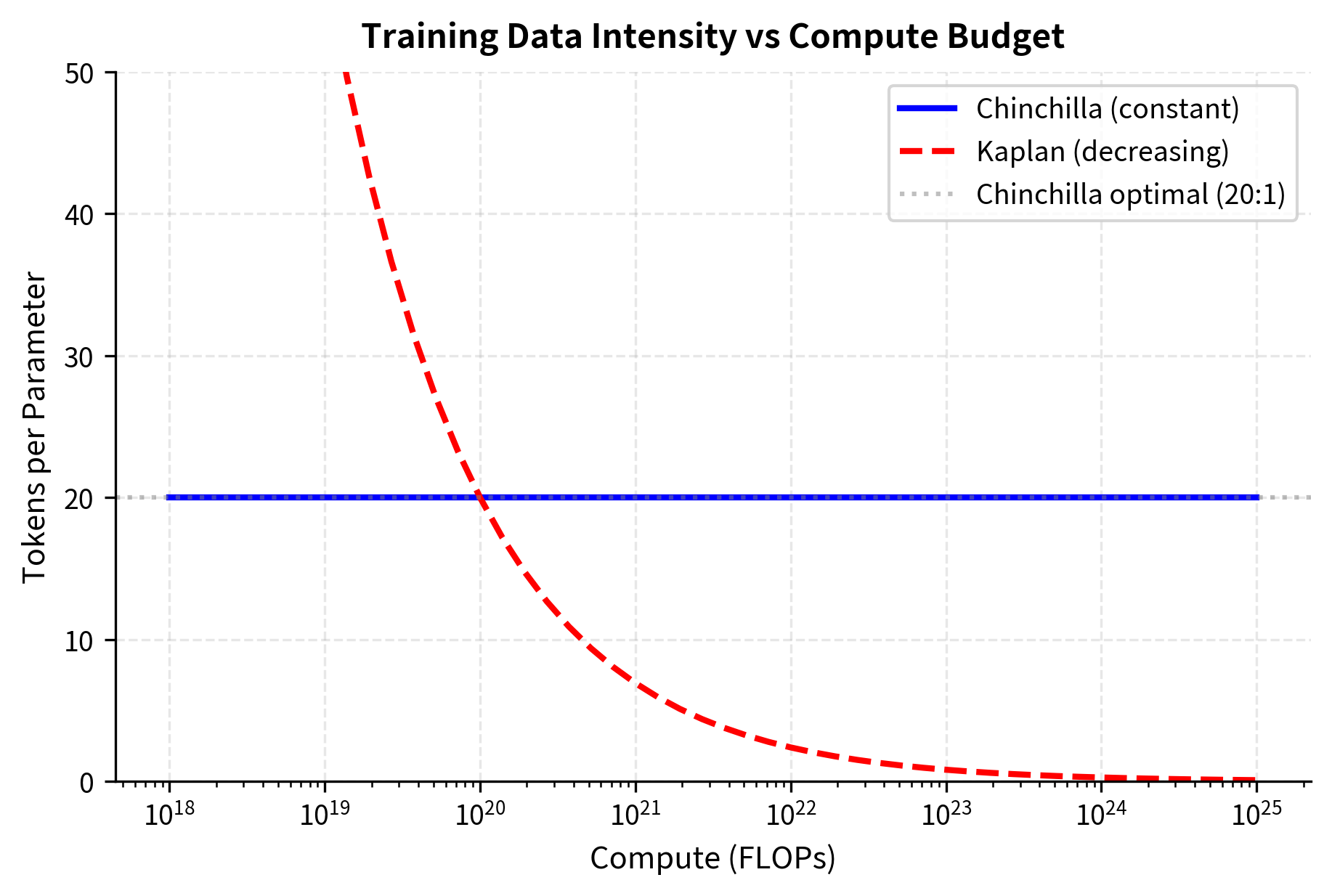
The flat blue line at 20 tokens per parameter represents the Chinchilla prescription: regardless of how much compute you have, maintain the same data intensity. The declining red line shows the problematic Kaplan implication: as compute grows, train on proportionally less data per parameter. At FLOPs, Kaplan scaling would suggest training on fewer than 5 tokens per parameter, a recipe for severe underfitting.
This visualization makes the fundamental difference clear: Chinchilla scaling maintains a constant data intensity regardless of scale, while Kaplan scaling implies training larger models on proportionally less data.
The Loss Surface Perspective
We can also visualize why balanced scaling is optimal by plotting the loss surface as a function of parameter count and token count for a fixed compute budget. This perspective offers geometric intuition for what the equations tell us algebraically. The optimal allocation lies not at the extremes but in a balanced middle region.
The loss function implemented above directly encodes the Chinchilla parametric form. Each call evaluates the predicted loss for a given parameter-token combination, allowing us to map out the loss landscape and identify where optimal performance lies.
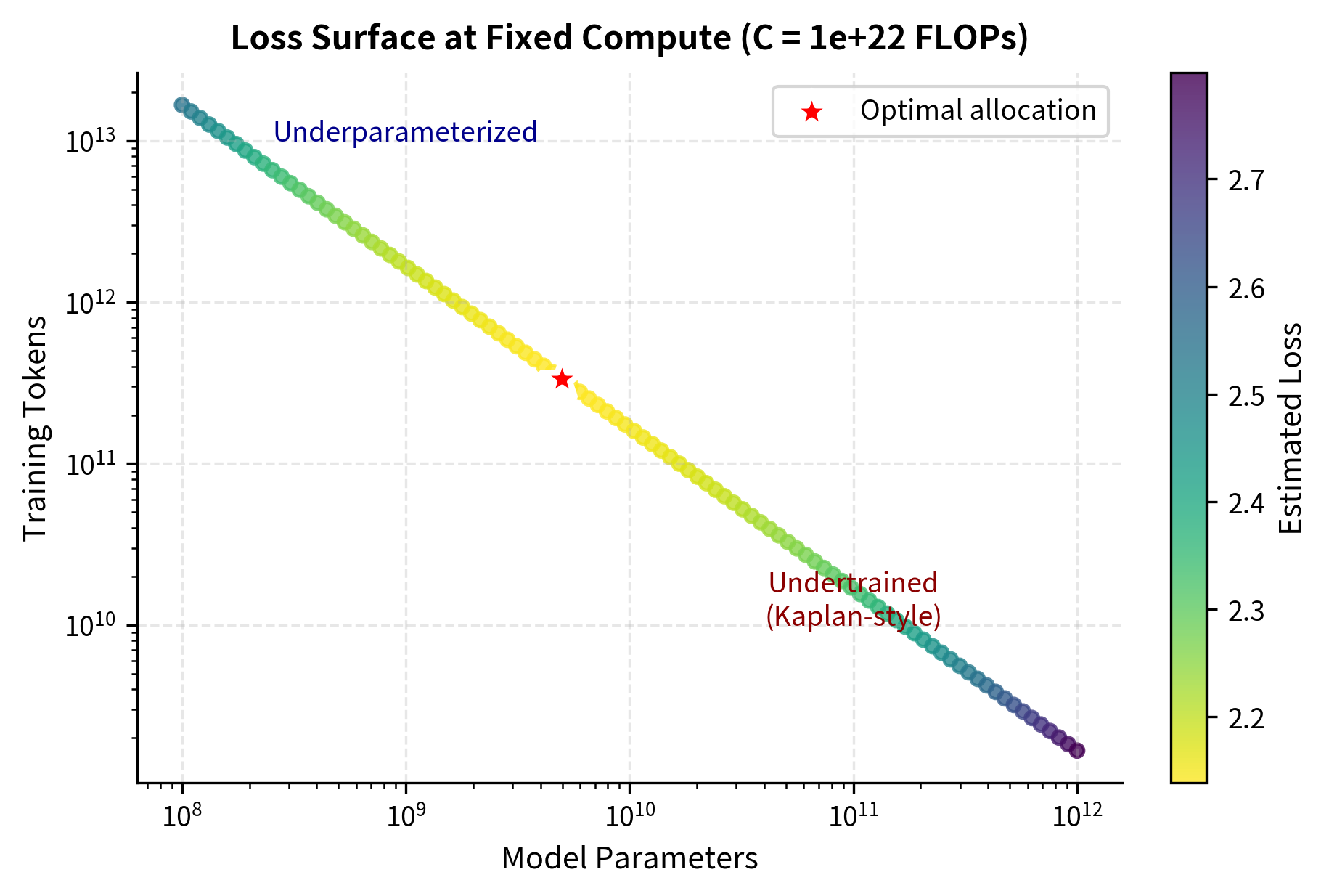
The computed optimal allocation of approximately 9B parameters and 180B tokens closely matches our earlier analytical calculation, validating the loss function approach. The estimated loss of around 2.0 nats represents a large reduction from what either extreme allocation would achieve. Moving toward the "Undertrained" region (upper left) or "Underparameterized" region (lower right) would increase loss significantly.
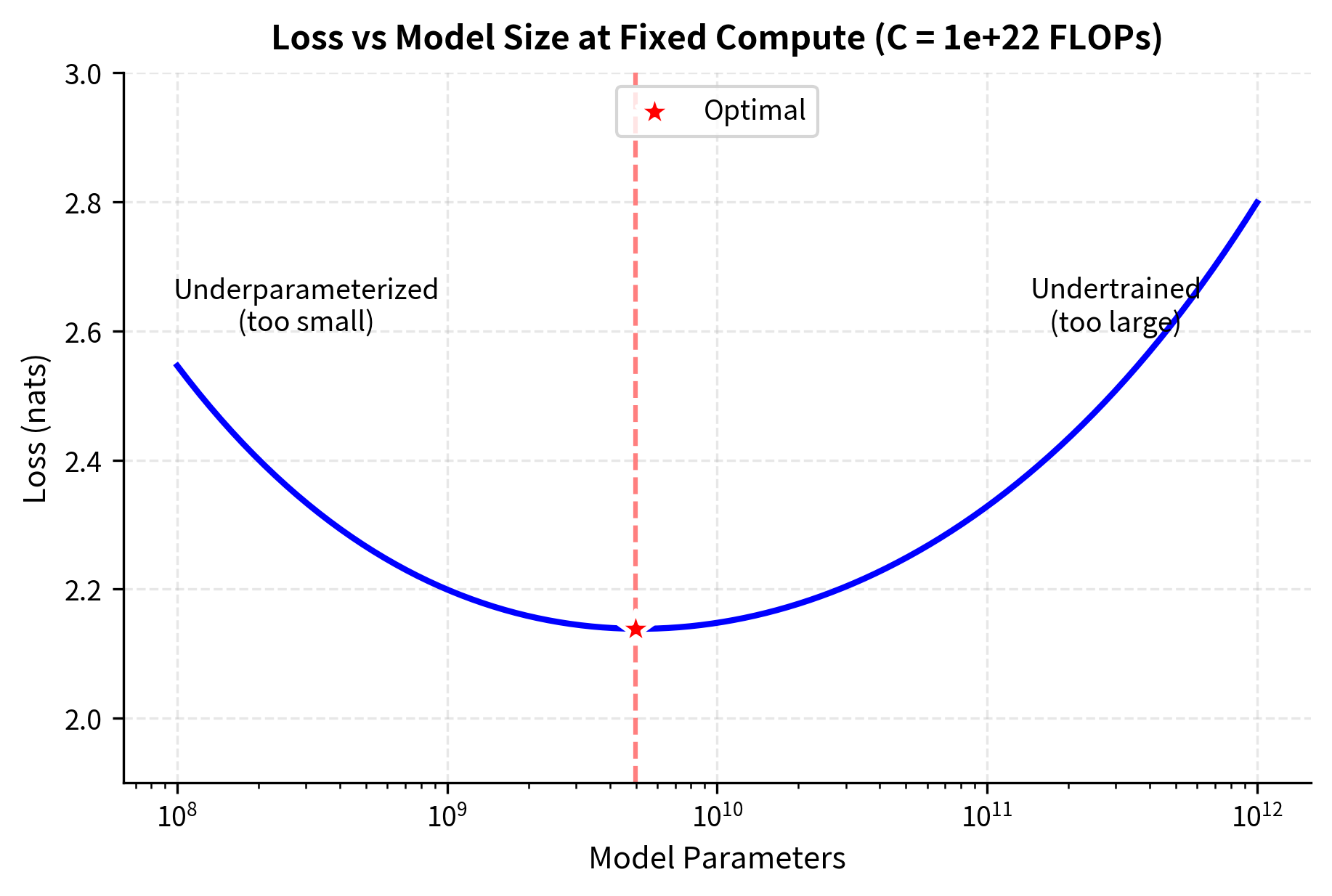
The optimal point lies in the balanced region, confirming the Chinchilla insight that neither extreme allocation (very large model with few tokens, or small model with many tokens) achieves the best performance. The loss surface visualization reveals the geometry underlying the scaling equations: the iso-FLOP curve traces out all possible ways to spend a fixed compute budget, and the optimal point marks where loss is minimized along this curve. The U-shaped loss profile along the curve shows that deviating in either direction, toward larger models or toward more data, incurs a penalty.
Key Parameters
The key parameters for Chinchilla scaling calculations are:
- compute_flops: Total compute budget in FLOPs, the primary input for determining optimal allocations
- tokens_per_param ratio (≈20): The Chinchilla-optimal ratio of training tokens to model parameters
- E, A, B, α, β: Fitted constants in the parametric loss function that determine the loss surface shape
- Scaling exponents (a, b ≈ 0.5): Exponents determining how optimal parameters and tokens scale with compute (, )
Caveats and Extensions
While Chinchilla scaling provides valuable guidance, several caveats apply.
The 20:1 Ratio Isn't Universal
The exact optimal ratio depends on data quality, model architecture, and training setup. Different analyses have found ratios ranging from 15:1 to 25:1. The key point is that the ratio should remain roughly constant across scales, not that 20:1 is precisely optimal for all situations.
Beyond Single-Epoch Training
The Chinchilla analysis assumes each token is seen once during training. When data is limited, multi-epoch training adds complexity. Repeated data provides diminishing returns, so the optimal strategy shifts toward smaller models. We'll explore this in detail in the upcoming Data-Constrained Scaling chapter.
Downstream Task Performance
Chinchilla scaling optimizes for pre-training loss, not necessarily downstream task performance. Some evidence suggests that larger models show emergent capabilities absent in smaller but better-trained models. The loss-capability relationship is not always linear, as we discuss in the chapter on Emergence in Neural Networks.
Inference Considerations
As noted earlier, Chinchilla scaling ignores inference costs. For models that will serve billions of queries, the accumulated inference cost may justify training a somewhat larger model to reduce the number of sequential operations at serving time. The upcoming Inference Scaling chapter addresses these trade-offs.
Limitations and Impact
The Chinchilla scaling laws changed how the field approaches language model development, but they come with important limitations worth understanding.
The most significant limitation is the focus on training compute while excluding other costs. While a Chinchilla-optimal 70B model achieves better loss than an undertrained 280B model for the same training compute, the larger model might be preferable if inference costs are negligible (for example, in research settings with limited deployment). The optimal allocation depends on the full lifecycle of the model, not just training.
Additionally, the Chinchilla analysis assumes access to unlimited unique training data. In practice, high-quality data is finite, and training on 20 tokens per parameter for a 100B+ model requires trillions of tokens. This has pushed the field toward synthetic data generation, multi-epoch training strategies, and careful data curation. These topics go beyond the scope of the original Chinchilla Using perplexity as the optimization target also has limits. Some capabilities appear to require model scale beyond what perplexity improvements would suggest. A 10B model trained to Chinchilla-optimal perplexity may still lack capabilities present in a 100B undertrained model, even if the smaller model has better loss. The relationship between loss and emergent capabilities is still an active research area.
Despite these limits, Chinchilla's impact has been significant. The paper showed that careful empirical analysis of scaling can overturn conventional wisdom and produce immediately useful insights. Labs rapidly adopted the 20:1 guideline, leading to models like LLaMA that achieve strong performance with far fewer parameters than GPT-3 era models. The shift toward data-efficient architectures and high-quality data curation traces directly to the Chinchilla insight that data matters as much as model size.
Summary
The Chinchilla scaling laws changed how we think about how to allocate compute between model size and training data. The key findings are:
- Balanced scaling: Model parameters and training tokens should grow at roughly equal rates as compute increases, not with the parameter-heavy allocation suggested by Kaplan
- The 20:1 ratio: Compute-optimal training uses approximately 20 tokens per parameter, meaning a 10B parameter model should see about 200B tokens
- Previous models were undertrained: GPT-3 and similar models trained on far fewer tokens per parameter than optimal, leaving performance gains unrealized
- Three independent methods: The Chinchilla team verified their findings using fixed model sizes, iso-FLOP curves, and parametric loss fitting, all yielding consistent results
The practical implications were immediate: smaller models trained on more data could match or exceed the performance of much larger undertrained models, while being cheaper to deploy. This shift toward compute-optimal training continues to influence model development, though new considerations around data constraints and inference scaling add detail to the original Chinchilla prescription.
Quiz
Ready to test your understanding? Take this quick quiz to reinforce what you've learned about Chinchilla scaling laws and compute-optimal training.

Comments