

Master SGD optimization for neural networks, including minibatch training, learning rate schedules, and how gradient noise acts as implicit regularization.

This article is part of the free-to-read Language AI Handbook
Choose your expertise level to adjust how many terms are explained. Beginners see more tooltips, experts see fewer to maintain reading flow. Hover over underlined terms for instant definitions.
Stochastic Gradient Descent
Training a neural network means finding weights that minimize a loss function. We've seen how backpropagation computes gradients, telling us which direction to move each weight to reduce the loss. But computing these gradients over an entire dataset is expensive. With millions of training examples, even a single gradient computation becomes prohibitively slow.
Stochastic Gradient Descent (SGD) solves this problem with a simple but powerful insight: we don't need perfect gradients. We just need gradients that point roughly in the right direction. By using small random samples instead of the full dataset, we trade precision for speed, often getting orders of magnitude faster training with minimal impact on the final result.
From Batch to Stochastic: The Core Idea
To understand why we need stochastic gradient descent, let's first examine what we're replacing and why the replacement works at all.
The Ideal: Computing the True Gradient
Imagine you want to know the average height of adults in a country. The most accurate approach is to measure everyone. Similarly, standard gradient descent, often called batch gradient descent, computes the loss gradient by averaging over every training example:
where:
- : the gradient of the total loss with respect to all model parameters
- : the total number of training examples in the dataset
- : the gradient computed from the -th training example alone
- : averaging factor that normalizes the sum
This formula computes the exact direction of steepest descent. Each training example contributes its own "opinion" about which way to adjust the weights, and averaging produces a consensus direction. The result is precise, but precision comes at a cost: you must process the entire dataset before taking a single optimization step.
For a dataset of one million images, that means one million forward passes, one million backward passes, and one million gradient computations, all before you can update a single weight. At this scale, batch gradient descent becomes impractical.
Batch gradient descent computes the gradient using the entire training set. This provides an accurate estimate of the true gradient direction but becomes computationally infeasible for large datasets.
The Insight: A Sample Can Substitute for the Population
Here's the key insight that makes stochastic gradient descent possible: you don't need to measure everyone to estimate the average.
Polling organizations don't survey every citizen; they sample a representative subset. The sample average is close to the true average, and more samples get you closer. The same logic applies to gradients. Instead of computing for all examples and averaging, what if we just... picked one example at random?
where:
- : the gradient computed from a single randomly selected training example
- : a random index, each value equally likely
This single-example gradient is an unbiased estimator of the true gradient. Mathematically, : if you average over all possible random choices, you get the exact batch gradient back. Any individual estimate might be wrong, perhaps dramatically so, but on average, it points in the right direction.
The tradeoff is variance for speed. A single-example gradient might point 45° away from the true direction, or even in the opposite direction for pathological examples. But it costs as much to compute. With a million examples, that's a million-fold speedup per gradient computation.
Visualizing the Tradeoff: Batch vs. Stochastic Gradients
Let's make this concrete. We'll create a simple linear regression problem and compare the batch gradient (computed from all 1000 examples) with stochastic gradients (each computed from a single example). The difference reveals exactly what we gain and what we sacrifice.
Now let's compute both types of gradients at the same point in parameter space and see how they compare:
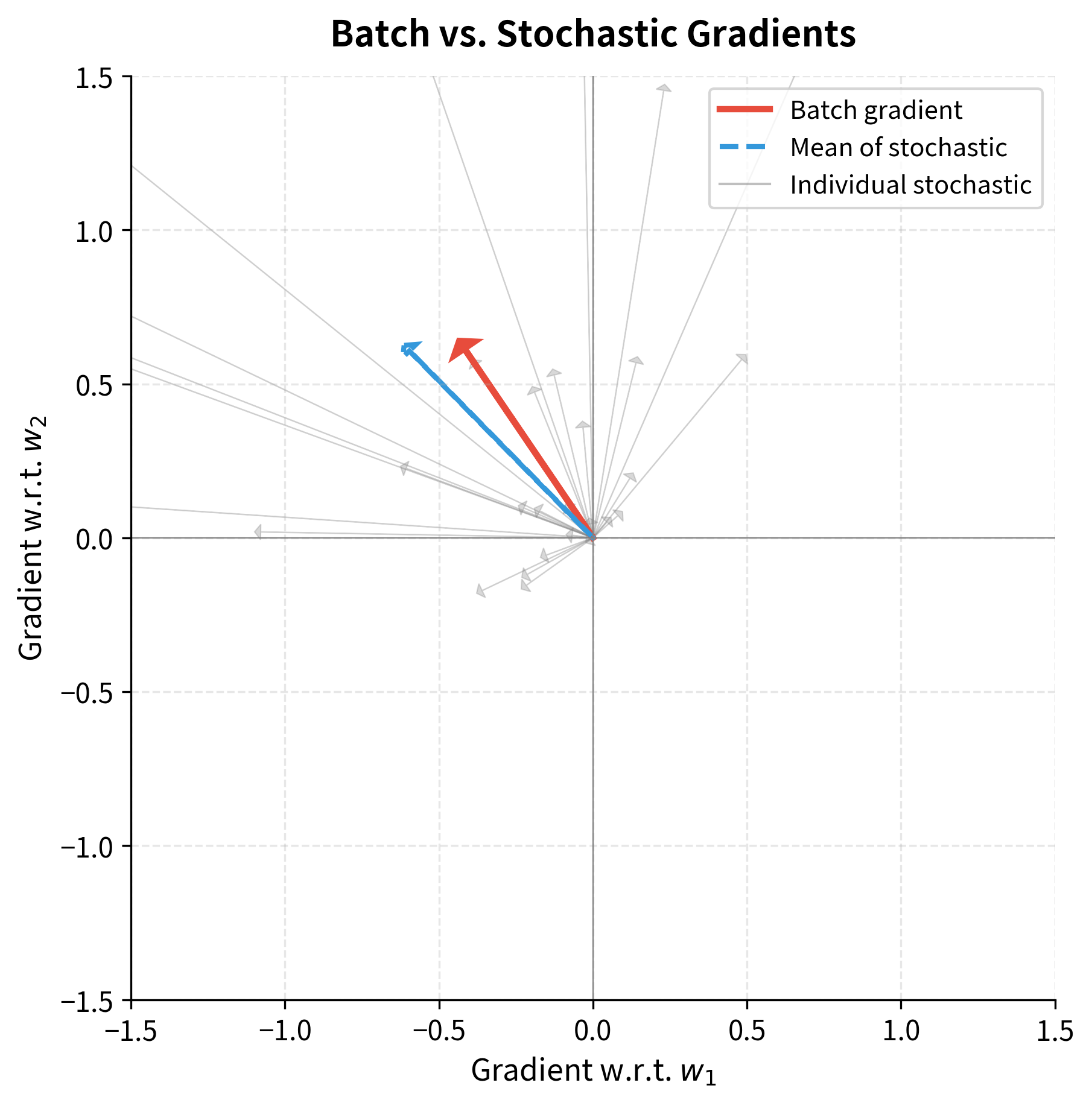
The visualization reveals the fundamental tradeoff at the heart of SGD. The batch gradient (red arrow) points precisely toward the optimum, getting the direction exactly right. The individual stochastic gradients (gray arrows) scatter wildly, some nearly orthogonal to the true direction, a few even pointing away from the optimum entirely. Any single gray arrow would be a poor substitute for the red one.
But look at the blue dashed arrow: the average of those scattered stochastic gradients. It aligns almost perfectly with the true batch gradient. This is not coincidence. It's the central limit theorem at work. Each stochastic gradient is an unbiased sample, so their average converges to the true gradient. The more samples you average, the closer you get.
This is the mathematical foundation of SGD: each step is imprecise, but the journey is correct on average.
The SGD Update Rule
Now that we understand why stochastic gradients work, let's formalize how we use them. At each iteration, SGD takes a step in the direction opposite to the gradient:
where:
- : the weight vector at iteration
- : the updated weight vector after iteration
- : the learning rate (step size), a positive scalar controlling how far we move
- : the gradient computed from a single randomly selected example
Understanding Each Component
Why subtract? Gradients point "uphill," toward increasing loss. Since we want to decrease the loss, we move in the opposite direction. Subtracting the gradient is moving downhill.
Why scale by ? The gradient tells us the direction, but not how far to go. The learning rate controls step size. Too small, and we inch toward the minimum over thousands of steps. Too large, and we overshoot, potentially bouncing around forever or diverging entirely. Finding the right is one of the most important (and frustrating) aspects of training neural networks.
Why use instead of ? This is what makes it stochastic. Using the full gradient gives batch gradient descent; using a single-example gradient gives pure SGD. The update formula is identical, only the gradient source changes.
The Training Loop: Epochs and Shuffling
In practice, we don't pick random examples with replacement. Instead, we shuffle the training set once, then iterate through every example in order. Once we've used every example once, that's one epoch. Then we shuffle again and repeat:
The results speak for themselves. SGD recovers weights extremely close to the ground truth, with the final loss dropping dramatically from its initial value. But here's the key insight: we made 1000 weight updates per epoch (one per training example), whereas batch gradient descent would make only one. Even though each SGD update is noisier than a batch update, we get 1000 chances to improve per epoch instead of just one.
This is why SGD often converges faster in wall-clock time despite being "noisier" per step. The total distance traveled toward the optimum per unit of computation is greater.
Visualizing the Optimization Path
Let's compare the actual trajectory through weight space for batch gradient descent vs. SGD. We'll run both starting from the same initial point and watch how they approach the optimum:
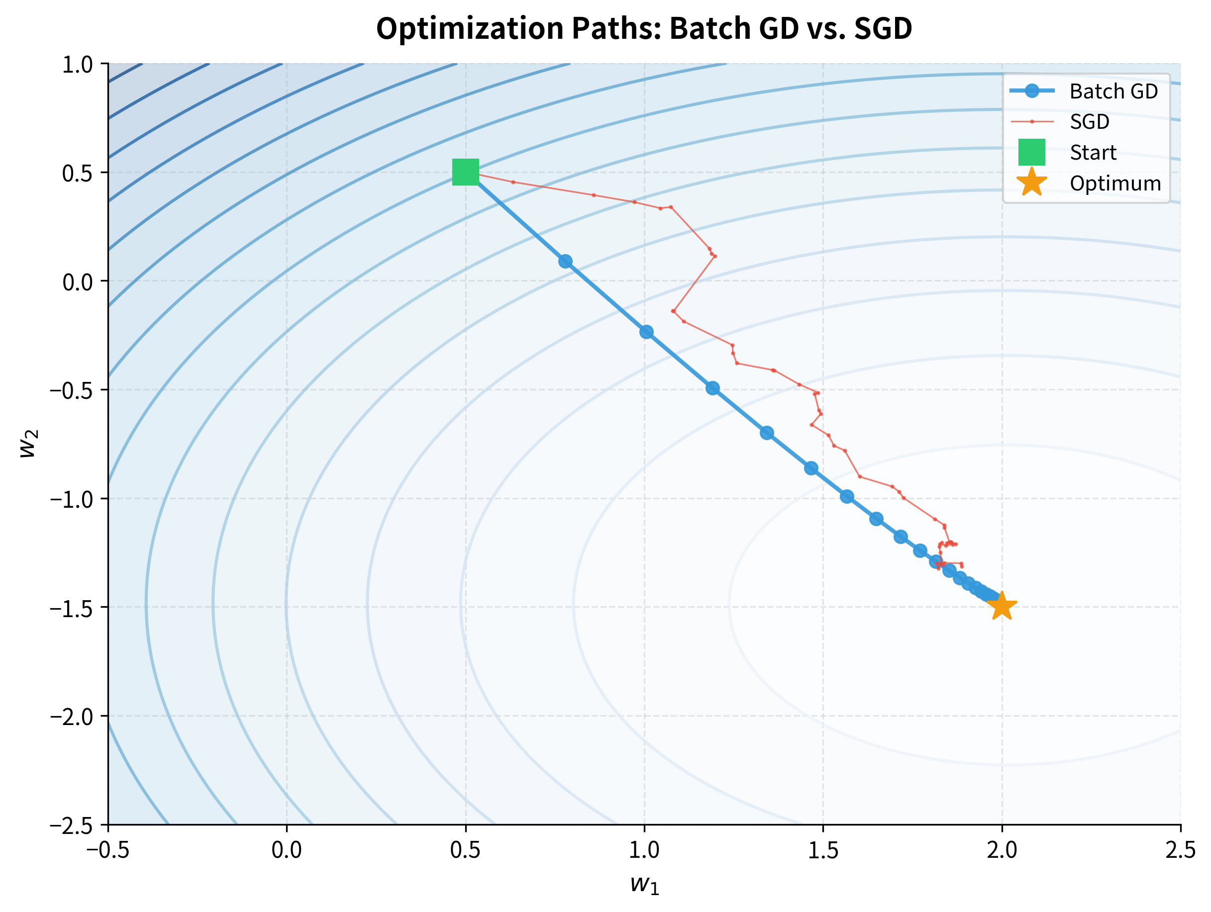
The visualization reveals the fundamental difference in how these methods explore the loss landscape. Batch gradient descent (blue) takes measured, deliberate steps directly toward the minimum, with each step using perfect information from the entire dataset. SGD (red) wanders drunkenly, zigzagging across the landscape as different training examples pull it in different directions.
Yet both reach the same destination. And despite its erratic path, SGD made many more updates in the same computational budget. This is the core tradeoff: precision vs. speed.
Minibatch Gradient Descent: The Best of Both Worlds
We've now seen two extremes:
- Batch gradient descent: Use all examples. Precise gradients, but one update per full dataset pass.
- Pure SGD: Use 1 example. Fast updates, but extremely noisy gradients.
In practice, neither extreme is ideal. Batch is too slow; pure SGD is too noisy and can't exploit modern hardware. The solution? Meet in the middle.
The Minibatch Compromise
Instead of all examples or just one, we use a small random subset, a minibatch, of examples:
where:
- : a minibatch, a random subset of training examples
- : the batch size (typically 32, 64, 128, or 256)
- : the gradient from the -th example in the minibatch
- : averaging factor that normalizes the sum
This is the same averaging formula as batch gradient descent, just applied to a smaller sample. If , we get batch gradient descent. If , we get pure SGD. For somewhere in between, we get the advantages of both:
- Reduced variance: Averaging over examples smooths out the noise. The variance of the gradient estimate decreases as .
- Efficient computation: GPUs are designed for parallel matrix operations. A minibatch of 64 examples can be processed almost as fast as a single example because the matrix multiplications happen in parallel.
- Practical balance: We still make updates per epoch (for 1000 examples and , that's about 31 updates), so we iterate quickly without extreme noise.
Minibatch gradient descent computes gradients using a small random subset of training examples (typically 32-256). This provides more stable gradients than pure SGD while maintaining computational efficiency.
Implementing Minibatch SGD
The implementation is nearly identical to pure SGD, but we process examples in groups rather than one at a time:
The key difference from pure SGD is in the loop structure: instead of iterating over individual indices, we iterate in steps of batch_size and slice out groups of examples. The gradient computation itself is unchanged; we just pass a matrix X_batch instead of a single row.
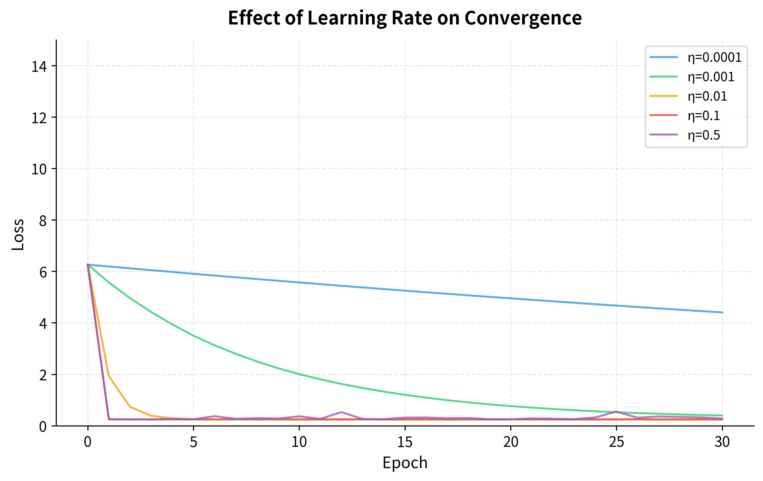
Let's compare how different batch sizes affect convergence:
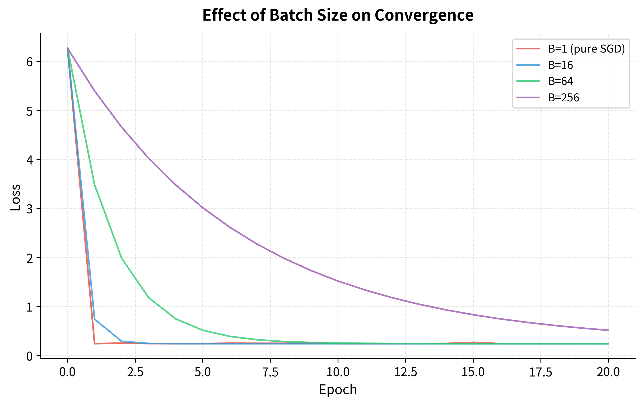
The curves reveal an illuminating pattern:
- Small batches (B=1, B=16) converge faster initially because they take more update steps per epoch, covering more ground early. But the path is jagged, reflecting high gradient variance.
- Large batches (B=64, B=256) are smoother, with less oscillation. But they make fewer updates per epoch, so early progress is slower.
- All reach similar final losses, given enough epochs. The journey differs, but the destination is the same.
This is the batch size tradeoff in action: more noise vs. more updates. Neither extreme is optimal, which is why batch sizes in the 32-256 range are the practical sweet spot.
Why These Specific Batch Sizes?
You'll notice that batch sizes are almost always powers of 2: 32, 64, 128, 256. This isn't superstition; it's hardware optimization. GPUs process data in parallel using memory layouts that align to powers of 2. A batch of 64 examples may process in the same time as a batch of 50, simply because 64 fits the hardware's natural granularity.
Beyond hardware, batch size affects learning dynamics:
- Too small (B < 16): Gradient variance is high, often requiring smaller learning rates to compensate. Training becomes erratic.
- Sweet spot (B = 32-256): Variance is reduced enough for stable training, while still making many updates per epoch. Memory usage fits comfortably on most GPUs.
- Too large (B > 1024): Diminishing returns on gradient quality (variance doesn't decrease much beyond a point), and research suggests very large batches may find sharper minima that generalize worse.
Updates per Epoch: The Hidden Tradeoff
Beyond noise, batch size affects how many times we update weights per epoch. Smaller batches mean more updates per pass through the data:
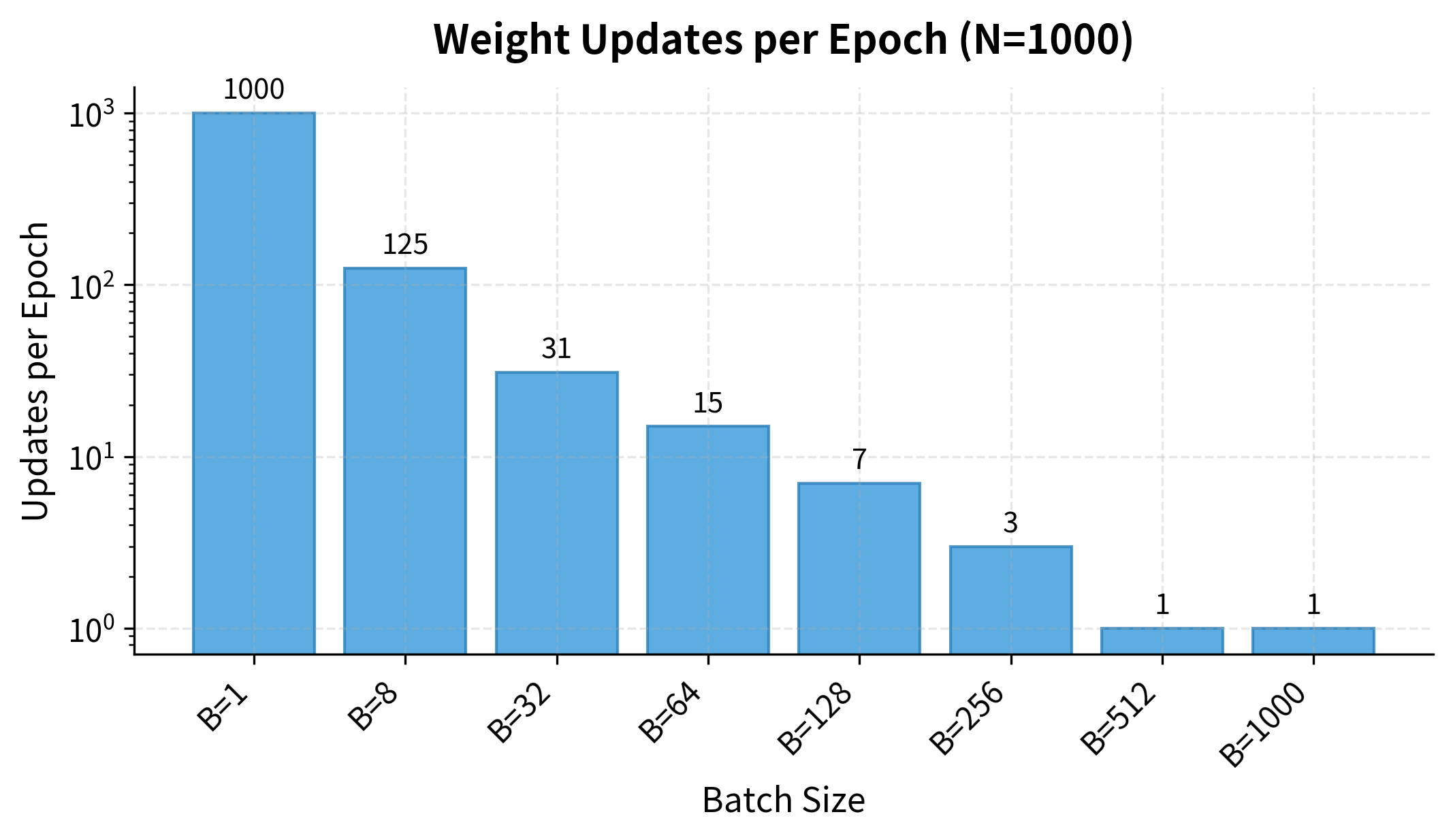
With batch size 1 (pure SGD), we make 1000 updates per epoch, one per example. With batch size 256, we make only about 4 updates. This is why small batches often converge faster in terms of epochs: each epoch does more optimization work. But each individual update is noisier, so the tradeoff isn't straightforward.
Quantifying the Variance Reduction
The central limit theorem predicts that gradient variance should decrease as : double the batch size, halve the variance. Let's verify this empirically:
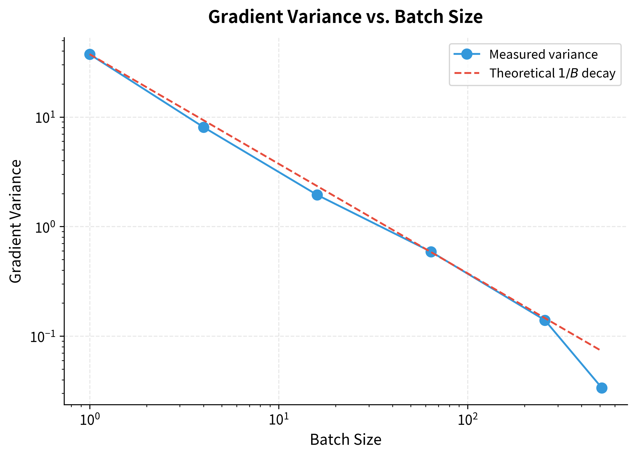
The log-log plot confirms the relationship: a straight line with slope -1. Doubling the batch size halves the variance, exactly as the central limit theorem predicts.
Let's visualize this variance reduction more intuitively by plotting the distribution of gradient estimates for different batch sizes:
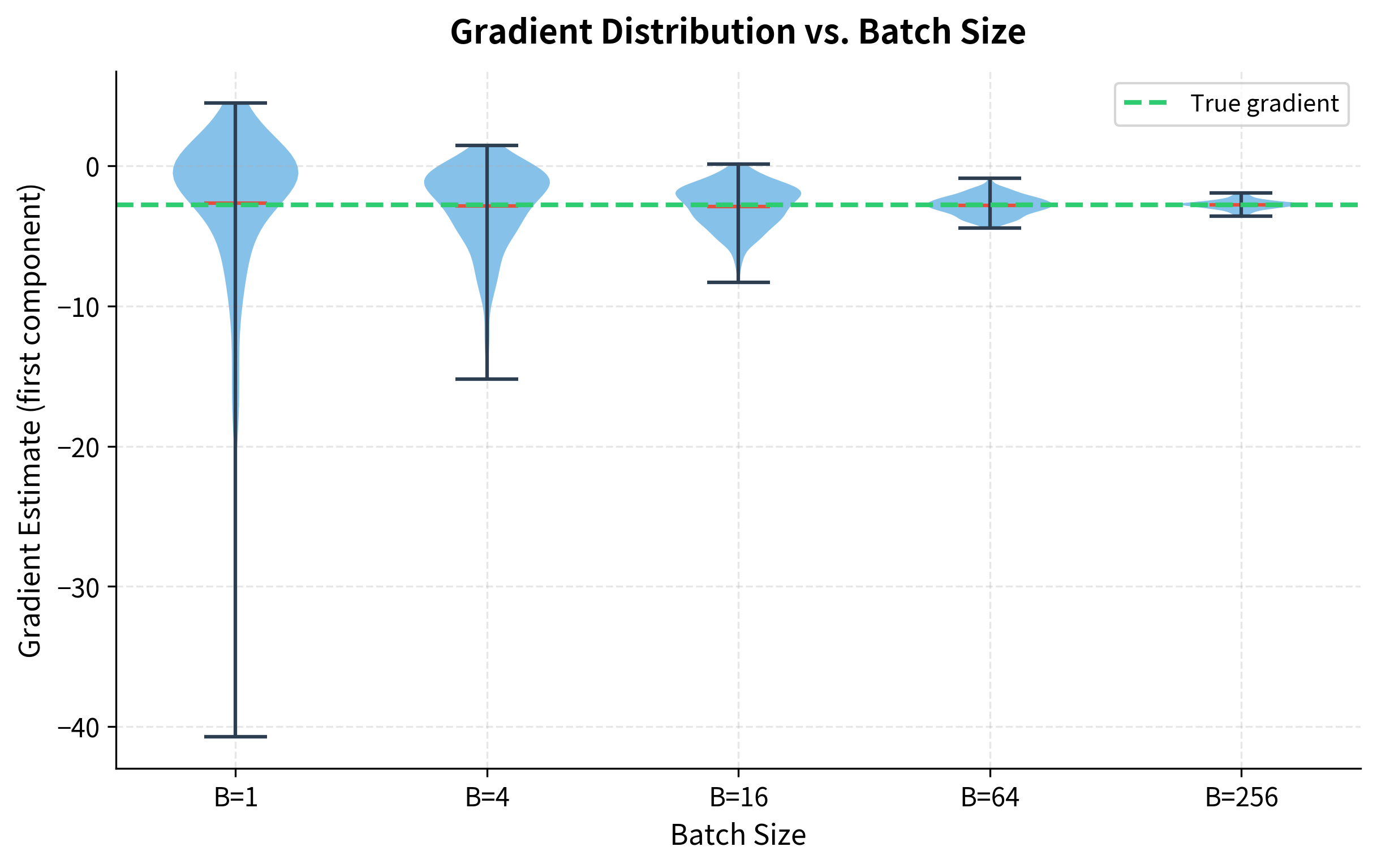
The violin plots make the variance reduction visceral. With B=1, gradient estimates scatter wildly, some far from the true value (green dashed line). As batch size increases, the distribution narrows dramatically. By B=256, estimates cluster tightly around the truth. This is why larger batches allow larger learning rates: the gradient you compute is much closer to the true direction.
This relationship has a profound practical consequence: if you double the batch size, you can often double the learning rate while maintaining training stability. The variance reduction from larger batches compensates for the larger steps. This "linear scaling rule" is widely used when training on multiple GPUs, where larger effective batch sizes are natural.
Learning Rate: The Critical Hyperparameter
We've discussed batch size as a dial we can tune. But the learning rate is the critical hyperparameter, the one that makes or breaks training. Get it wrong, and your model either learns nothing or explodes.
The Goldilocks Problem
Unlike batch size, where 32-256 usually works fine, learning rate is problem-specific. A value that works perfectly for one model might cause another to diverge. Here's what happens at different settings:
-
Too small (): Each step is a timid shuffle toward the minimum. Training is stable and won't diverge, but it's glacially slow. You might need thousands of epochs to converge, and you may get stuck in shallow local minima along the way.
-
Just right (): Each step makes meaningful progress without overshooting. The loss decreases steadily, and you reach a good solution in a reasonable number of epochs.
-
Too large (): Each step overshoots the minimum, landing on the other side of the valley. The next step overshoots again. The loss oscillates wildly, or worse, increases exponentially until numerical overflow kills training.
Finding the right learning rate manually is tedious. The learning rate finder technique automates this by sweeping across learning rates and tracking when the loss starts increasing:
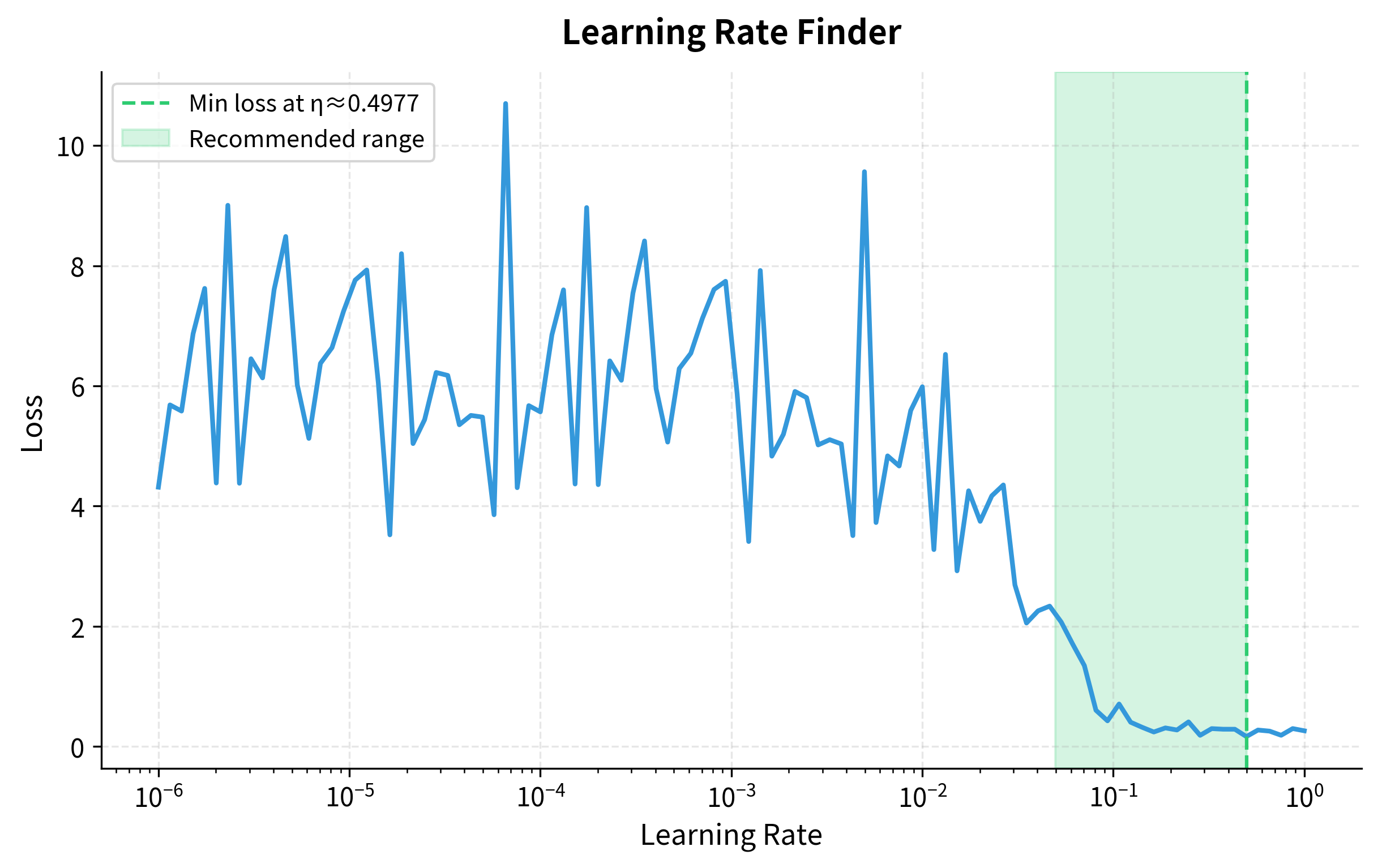
The plot shows the classic learning rate finder shape: loss decreases as we increase the learning rate (we're making meaningful progress), then suddenly shoots up when the rate gets too large (we're overshooting). The optimal learning rate is typically 1-10× smaller than where the loss starts increasing, around 0.01-0.05 in this case. This technique, popularized by Leslie Smith, can save hours of manual tuning.
SGD Convergence Properties
We've seen that SGD trades exact gradients for speed. But does this tradeoff come at a cost to where we end up? Understanding SGD's convergence behavior reveals both its power and its subtleties.
The Noisy Path to Convergence
Batch gradient descent, with exact gradients, descends smoothly to the minimum. Each step moves directly downhill, and if the learning rate is small enough, the algorithm converges to a fixed point.
SGD is different. With a constant learning rate, SGD never converges to a point. It oscillates around the minimum, bouncing in a region whose diameter is proportional to . The gradient noise prevents it from settling.
This might seem like a fundamental flaw, but it's actually a consequence of a tradeoff. To guarantee exact convergence, we need a decaying learning rate that satisfies two mathematical conditions:
where:
- : the learning rate at iteration
- : the cumulative sum of all learning rates
These conditions may seem abstract, but they encode a precise balance:
-
First condition (): We must be able to travel unbounded total distance. If learning rates decay too fast, like , the sum converges to a finite value, and we might stop moving before reaching the minimum. The algorithm gets "stuck" because it runs out of step budget.
-
Second condition (): The accumulated variance must be bounded. Each SGD step has variance proportional to (from the noisy gradient). If this sum diverges, we bounce around forever, never settling down.
A schedule like threads this needle: it decays slowly enough that the sum diverges (we can always reach the goal), but fast enough that the sum of squares converges (we eventually stop bouncing).
From Theory to Practice: Learning Rate Schedules
In practice, few practitioners use theoretically-motivated schedules like . Instead, empirically-tuned schedules dominate. The key insight is that we want large steps early (when we're far from the optimum and any progress is good) and small steps late (when we're near the optimum and need precision).
Let's implement and compare several common schedules:
We define four schedules representing different decay philosophies:
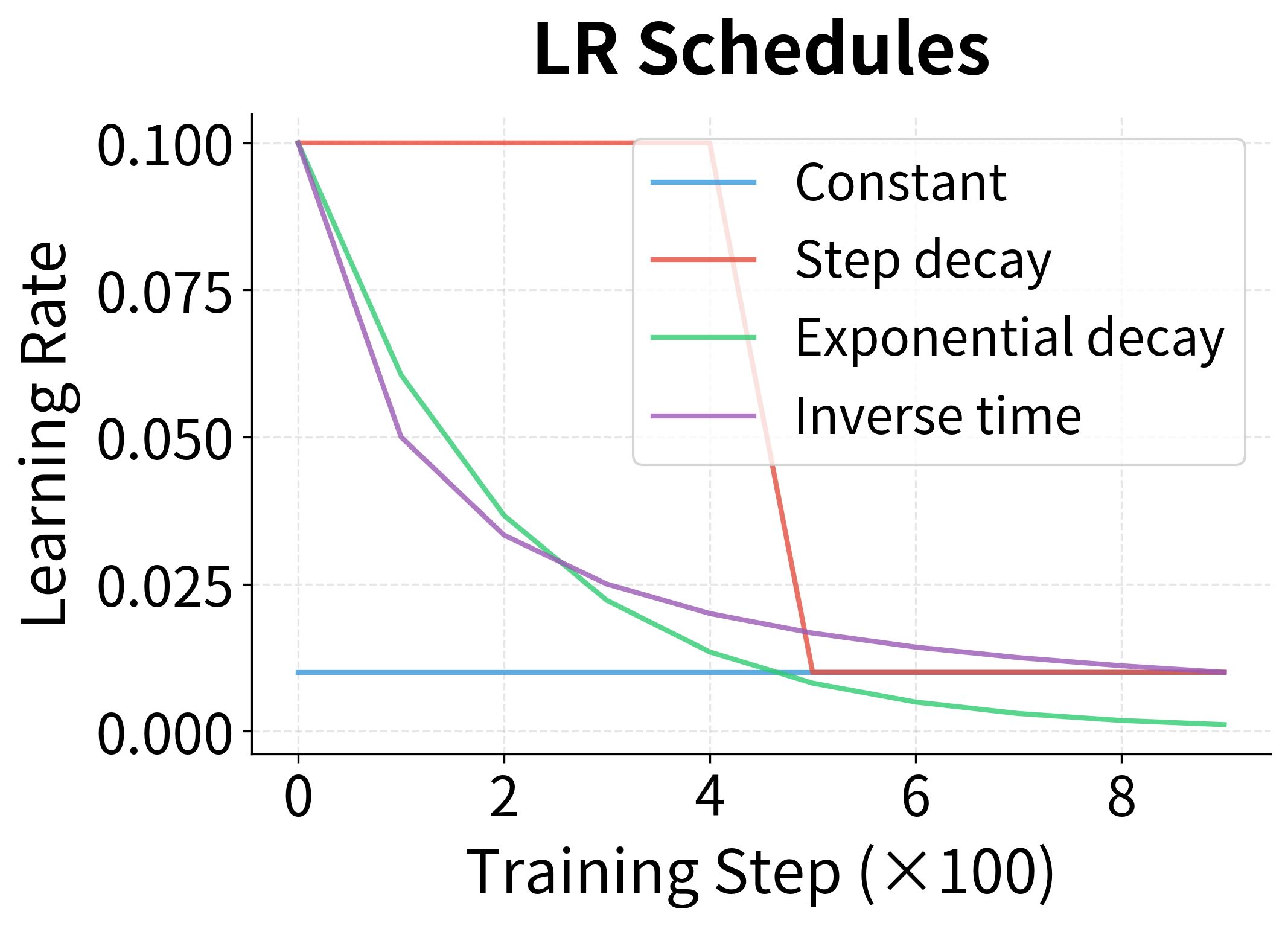
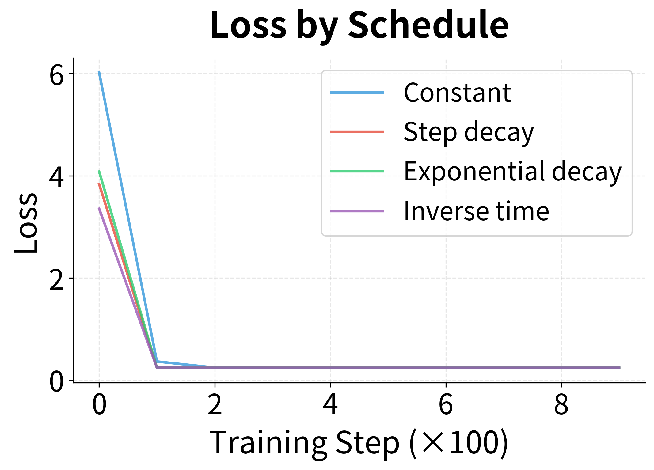
The left plot shows how each schedule reduces the learning rate over training steps. The constant schedule stays flat; step decay has sharp drops; exponential and inverse-time decay smoothly.
The right plot reveals the consequence: decaying schedules achieve lower final losses. The constant schedule converges quickly but then oscillates because it can't settle precisely into the minimum with such large steps. The decaying schedules take big steps early (making fast initial progress) then small steps late (settling precisely into the minimum).
Common Learning Rate Schedules in Practice
Several schedules have become standard, each with particular strengths:
| Schedule | Formula | Use Case |
|---|---|---|
| Step decay | Most common; drop by factor every steps | |
| Exponential | Smooth decay; can be too aggressive | |
| Cosine annealing | Popular for vision models; smooth with warm restarts | |
| Linear warmup | Increase linearly for first steps, then decay | Essential for transformers; prevents early instability |
In these formulas:
- : learning rate at step
- : initial learning rate
- : decay factor (typically 0.1 for step decay, 0.99-0.999 for exponential)
- : step interval for step decay
- : total number of training steps for cosine annealing
- : minimum learning rate (floor for cosine schedule)
- : number of warmup steps
Let's visualize all these schedules together, including cosine annealing and warmup:
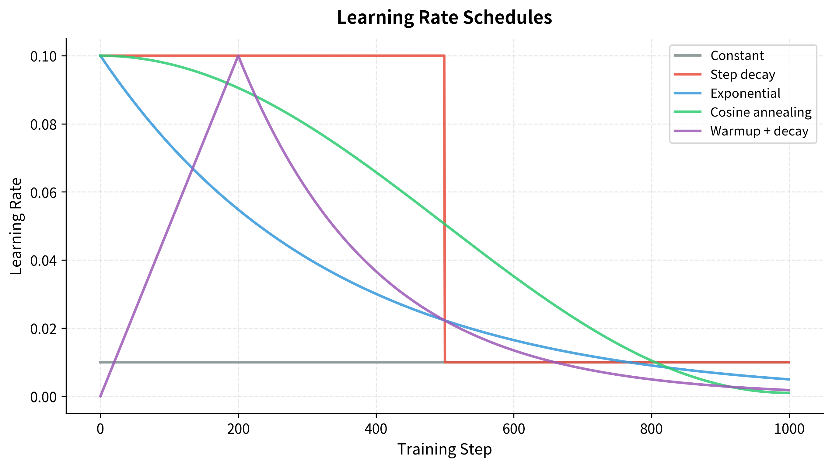
The choice of schedule often matters less than having a schedule. The key is reducing the learning rate as training progresses; the specific shape is secondary. That said, each schedule has its niche:
- Cosine annealing is particularly popular for training vision models, as the smooth curve avoids sudden drops that can destabilize training
- Warmup is essential for transformers and models with layer normalization, preventing early training instability
- Step decay remains the workhorse for many applications, offering predictable drops at known epochs
SGD Noise as Implicit Regularization
Everything we've discussed so far treats SGD's noise as a necessary evil, the cost of speed. But here's a surprising fact: the noise actually helps generalization. What looks like a bug is actually a feature.
The Generalization Puzzle
Consider two training runs that achieve the same final loss on the training set. Both fit the data equally well. Yet one might generalize better to new data than the other. Why?
The answer lies in where they ended up in the loss landscape, not just how low they got.
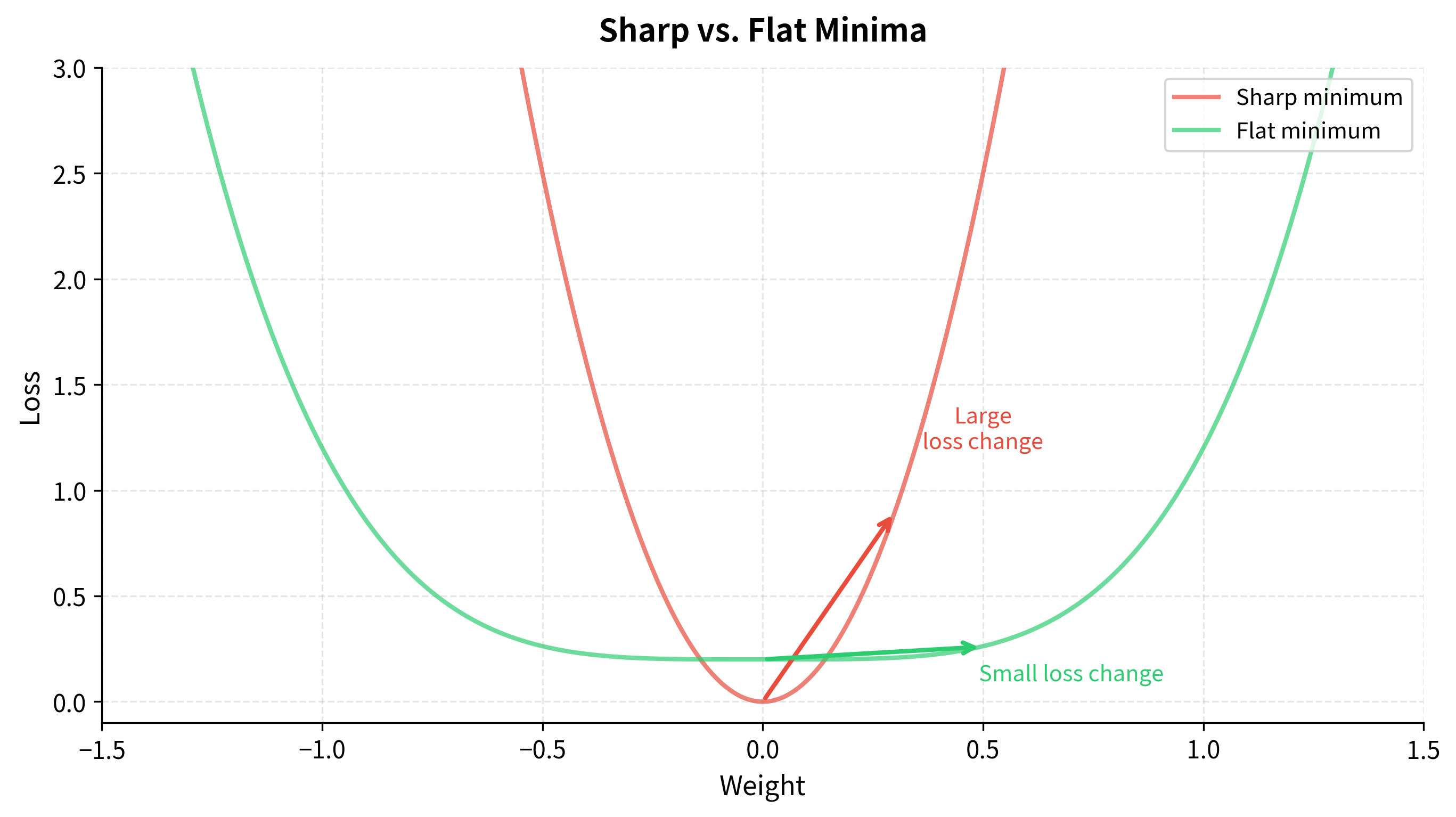
Sharp vs. Flat Minima
Neural network loss landscapes have many local minima, perhaps exponentially many. Some are sharp: the loss increases steeply as you move away from the minimum in any direction. Others are flat: the loss changes gradually, creating a broad basin.
Research suggests that flat minima generalize better. The intuition is straightforward: test data comes from a slightly different distribution than training data. This shifts the loss landscape slightly. If you're in a sharp minimum, even a small shift might push you up a steep wall, dramatically increasing loss. If you're in a flat minimum, the same shift barely matters because you're still near the bottom of a broad basin.
How SGD Noise Finds Flat Minima
Here's where SGD's noise becomes a feature rather than a bug. The gradient noise has a specific structure: it depends on the local curvature of the loss.
Near sharp minima with high curvature, gradient variance is high. The loss changes rapidly in all directions, so different training examples disagree sharply about which way to go. This disagreement translates to noisy, high-variance gradients.
Near flat minima with low curvature, gradient variance is low. The loss is nearly constant in the neighborhood, so all examples agree: "we're in a good spot." Gradients are small and consistent.
The consequence? SGD naturally bounces out of sharp minima while settling into flat ones. The noise is proportional to curvature, so sharp minima are inherently unstable under SGD dynamics.
This relationship can be quantified. The effective noise scale in SGD, measuring how much the optimization path fluctuates, is approximately:
where:
- : the learning rate (step size)
- : the batch size (number of examples per gradient computation)
- : the variance of per-example gradients
- : the noise-to-signal ratio of each update
Larger steps () amplify the noise, while larger batches () reduce it through averaging. The ratio controls the net noise level. This explains several well-known empirical observations:
- Smaller batches → better generalization: More noise helps bounce out of sharp minima into flatter ones
- Larger learning rates → better generalization (up to a point): Same mechanism, more exploration
- The ratio matters more than either alone: Doubling batch size while doubling learning rate maintains similar dynamics
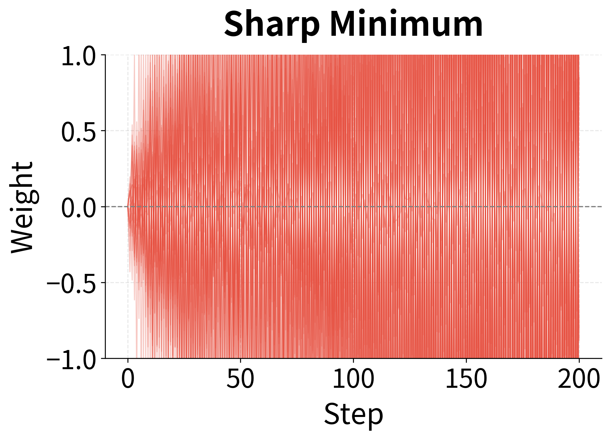
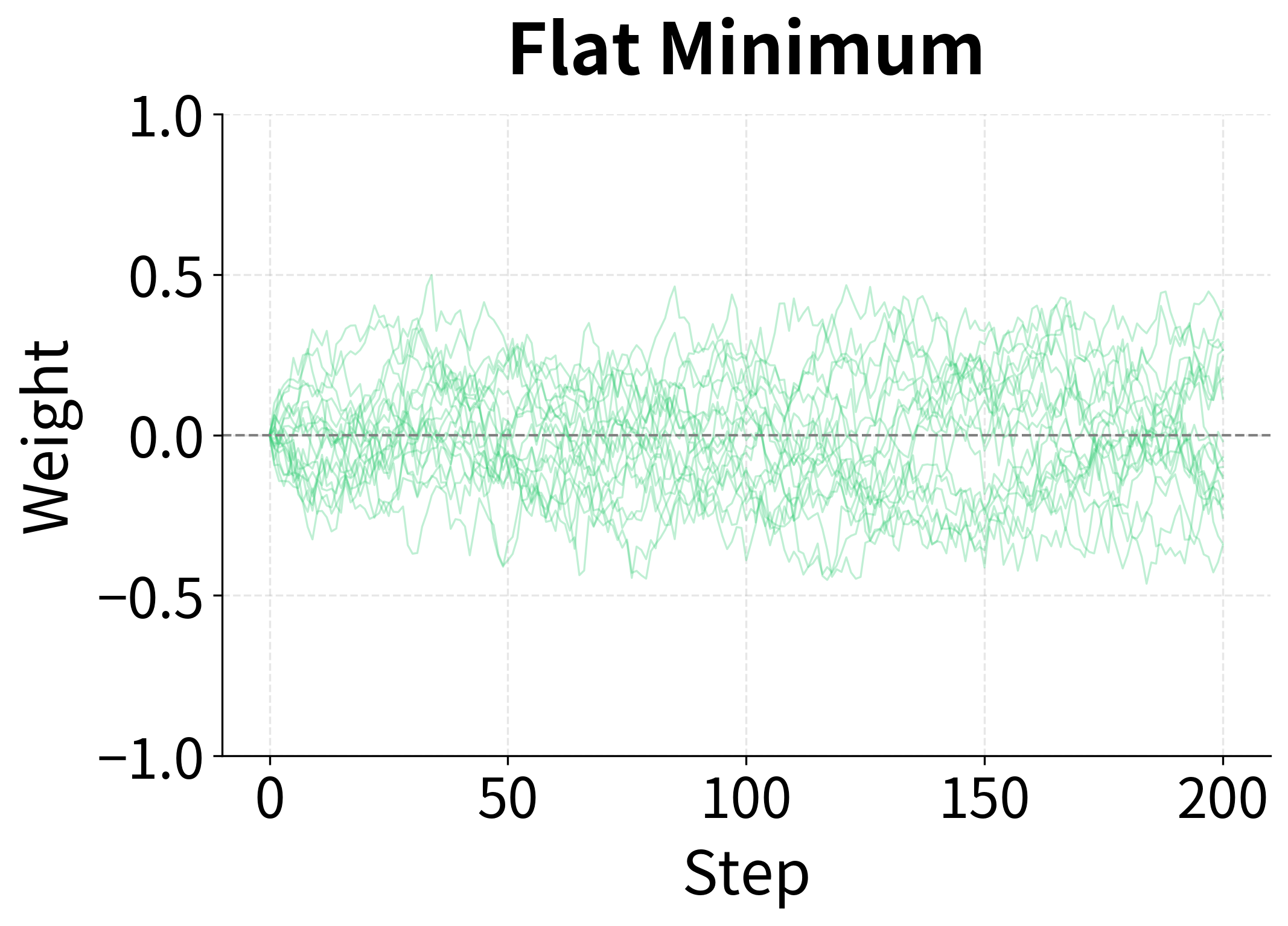
The contrast is striking. In the sharp minimum (left), SGD oscillates wildly because the high curvature creates high gradient variance, and the optimizer bounces around forever. In the flat minimum (right), SGD converges stably because the low curvature means low variance, and the optimizer settles down.
This isn't a flaw to be fixed; it's a feature to be exploited. The noise in SGD naturally selects for solutions that generalize well.
A Worked Example: Training a Classifier
We've explored SGD's mechanics through linear regression, a convex problem where the theory is clean. Now let's bring everything together with a more realistic example: training a neural network classifier from scratch using SGD. This will show how batch size, learning rate, and schedules interact when the loss landscape is non-convex.
The Dataset and Model
We'll use the "moons" dataset: two interleaved crescent shapes that require a nonlinear decision boundary. A simple 2-layer neural network with ReLU activations will learn to separate them.
The neural network implements the forward pass (input → hidden → output), the backward pass (computing gradients for each weight), and weight updates. The loss method computes binary cross-entropy, and accuracy measures classification performance.
Training with SGD
Now let's train this network with SGD, comparing constant vs. decaying learning rates:
Both configurations achieve strong test accuracy, and our simple 2-layer network successfully separates the crescents. The generalization gap (train minus test accuracy) is small, indicating the models are not overfitting. Learning rate decay achieves slightly better final performance by taking smaller steps as training progresses, allowing finer adjustments near the optimum.
Visualizing the Learning Process
Let's examine the training dynamics more closely:
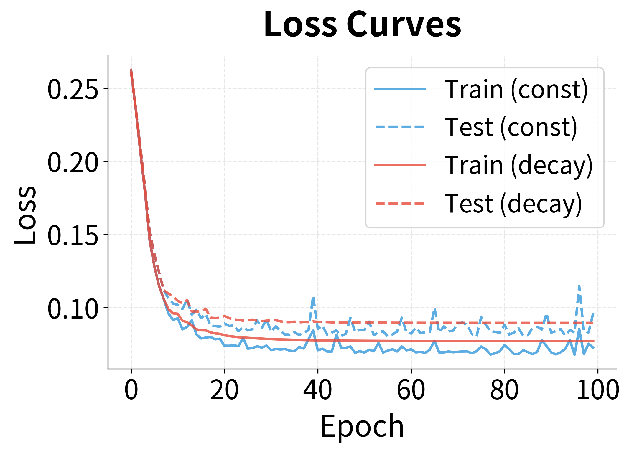
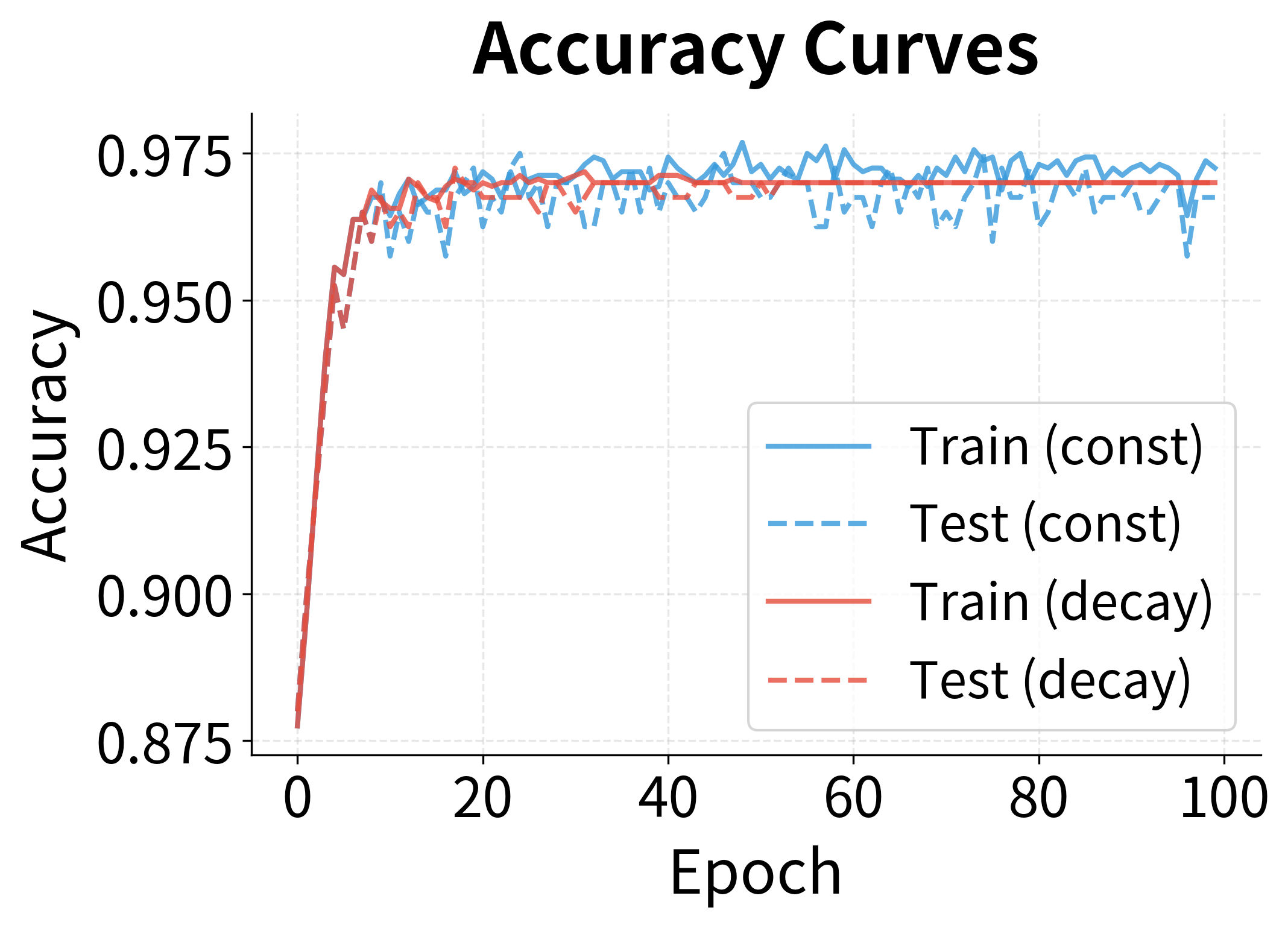
The loss curves show a familiar pattern: rapid initial decrease followed by slower refinement. The learning rate decay schedule (red) achieves lower final loss because it can take more precise steps late in training. The accuracy curves show corresponding behavior, with both reaching high accuracy quickly, though the decaying schedule achieves slightly better final values.
The Learned Decision Boundary
Finally, let's visualize what the network actually learned: the decision boundary separating the two classes.
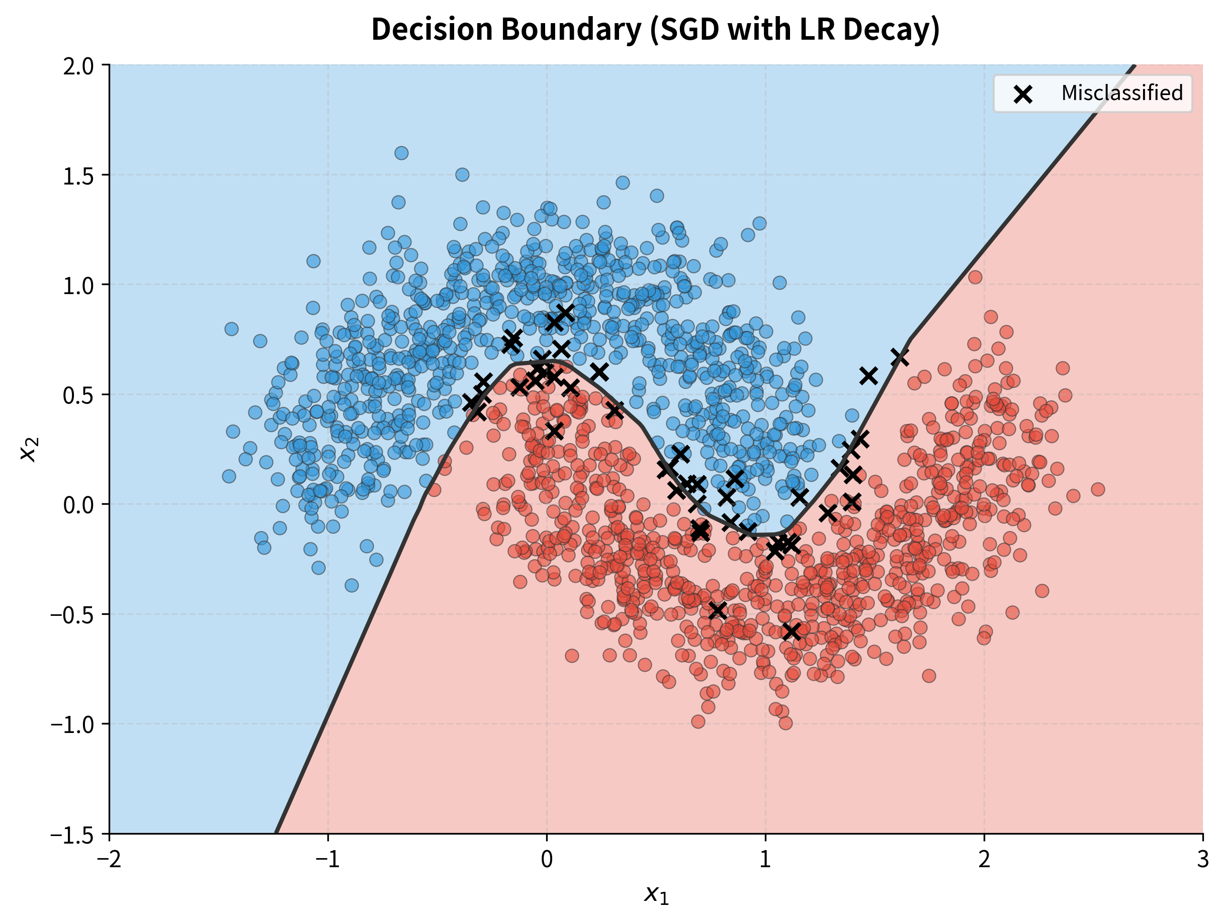
The network learned a smooth, curved boundary that follows the natural shape of the moons. Correctly classified points appear as circles; the rare misclassified points (near the boundary where the classes overlap) appear as X markers. SGD with learning rate decay found weights that generalize well. The boundary isn't overfit to individual training points but captures the underlying pattern.
Complete SGD Implementation
Having explored SGD's theory and applications, let's consolidate everything into a reusable implementation. This SGDOptimizer class encapsulates the key components: learning rate scheduling and minibatch generation.
The class has three main responsibilities:
get_lr(): Returns the current learning rate, applying the schedule if one is providedstep_update(params, gradients): Applies the SGD update rule:create_batches(X, y): Generates shuffled minibatches for one epoch
Here's how you would use the optimizer in a training loop:
The optimizer handles learning rate scheduling internally, so you don't need to manually track the step count. The create_batches method yields shuffled minibatches, ensuring each epoch sees the data in a different order (important for avoiding cyclic patterns that can hurt convergence).
Limitations and Challenges
SGD is remarkably effective. It's trained virtually every neural network you've ever used. But it has well-known limitations that motivate the more sophisticated optimizers we'll study next.
One Learning Rate for All Dimensions
The "optimal" learning rate varies across different dimensions of the parameter space. Dimensions with large gradients (steep loss surface) want small learning rates to avoid overshooting. Dimensions with small gradients (gentle slope) want large learning rates to make meaningful progress.
Vanilla SGD uses the same for all dimensions. This is a fundamental mismatch: the learning rate that works for steep dimensions is too small for gentle ones, and vice versa.
Difficulty with Saddle Points
In high-dimensional spaces, saddle points (where gradients are zero but it's not a minimum) are far more common than local minima. Near a saddle point, gradients become tiny, and SGD slows to a crawl. The optimizer might spend thousands of iterations in the "saddle" region before random noise eventually pushes it over the edge.
Oscillation in Ill-Conditioned Problems
When the loss surface is elongated, with high curvature in some directions and low curvature in others, SGD exhibits a characteristic pathology: it oscillates rapidly across the narrow valley while making slow progress along the long axis.
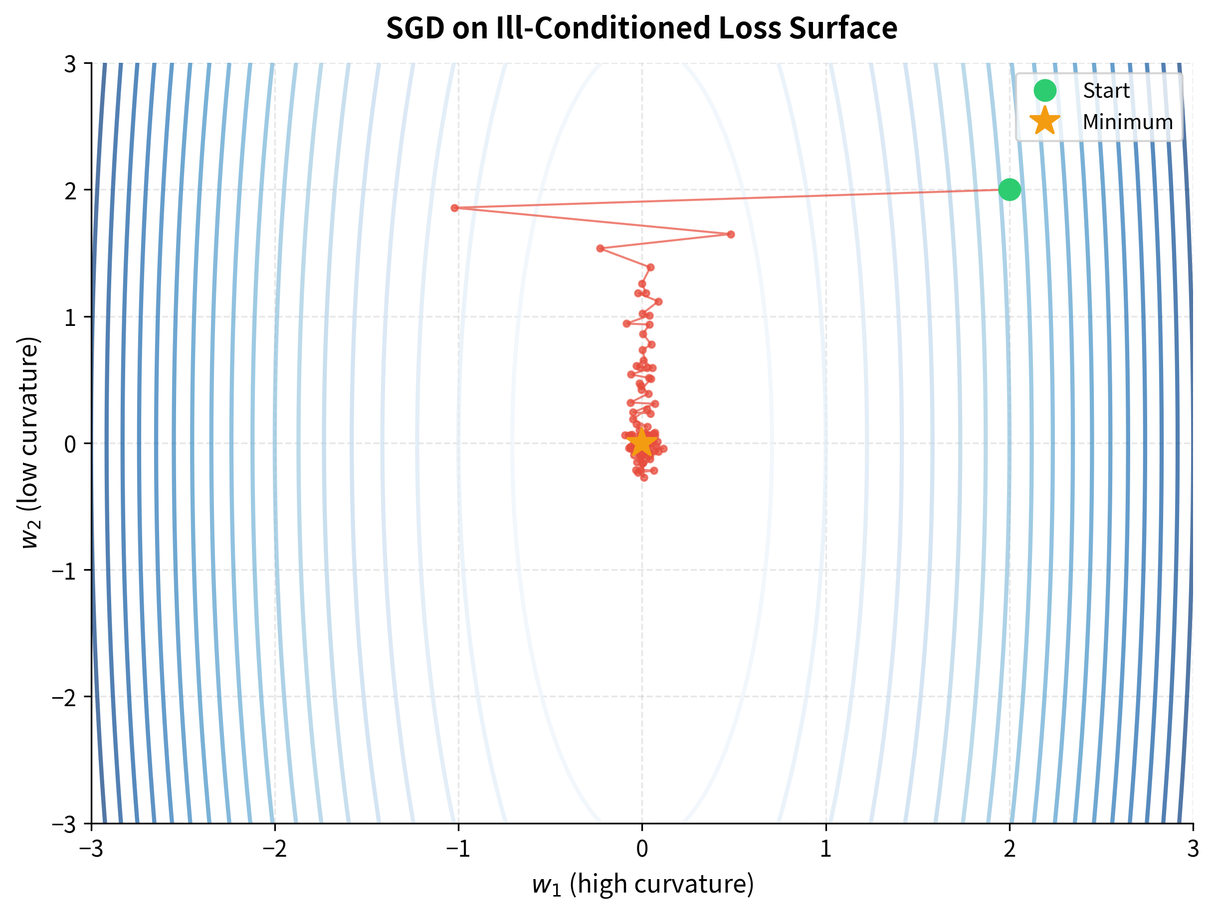
The oscillation pattern is unmistakable. In the steep direction (, horizontal axis), SGD overshoots repeatedly, bouncing back and forth across the valley. In the shallow direction (, vertical axis), it makes painfully slow progress because the gradients are small.
This is an ill-conditioned problem, where the ratio of largest to smallest curvature is high. For vanilla SGD, ill-conditioning is poison. The learning rate that's appropriate for the steep direction is far too small for the shallow one.
These limitations motivate momentum-based methods, which we'll explore in the next chapter. By accumulating a "velocity" that builds up along consistent gradient directions, momentum methods dampen the oscillations while accelerating progress along the valley floor.
Summary
Stochastic Gradient Descent trades exact gradients for speed, making neural network training practical at scale. The key ideas:
Core mechanics:
- Batch gradient descent uses all data for each update; computationally expensive but precise
- Pure SGD uses single examples; fast but noisy
- Minibatch SGD (the practical choice) uses small batches (32-256), balancing speed and stability
Learning rate:
- Too small: training is slow but stable
- Too large: training is fast but may diverge
- Learning rate finder helps identify a good starting point
- Decaying schedules (step, exponential, cosine) improve final convergence
Noise as regularization:
- SGD noise helps escape sharp minima that generalize poorly
- Smaller batches and larger learning rates increase effective noise
- The ratio controls the noise scale
Practical considerations:
- Shuffle data each epoch to avoid cycles
- Monitor both training and validation loss
- Use learning rate schedules for best convergence
- Gradient variance decreases as with batch size
SGD's limitations, sensitivity to learning rate, slow convergence on ill-conditioned problems, and difficulty with saddle points, motivate the momentum-based optimizers we'll explore in the next chapter.
Key Parameters
| Parameter | Typical Values | Effect |
|---|---|---|
| Learning rate () | 0.001-0.1 | Higher values mean faster but less stable training |
| Batch size () | 32-256 | Larger batches reduce gradient variance but may hurt generalization |
| Epochs | 50-500 | More epochs allow more updates; use early stopping to prevent overfitting |
| Learning rate decay | 0.1-0.5 every N steps | Enables convergence to precise minima |
When starting with a new problem, a reasonable baseline is:
- Batch size: 32 or 64
- Learning rate: Use a learning rate finder, or start with 0.01
- Schedule: Step decay by 0.1 every 30% of total training
- Shuffle: Always shuffle data each epoch
Quiz
Ready to test your understanding? Take this quick quiz to reinforce what you've learned about stochastic gradient descent and optimization.

Comments