Batch Normalization: Stabilizing Deep Network Training

Training deep neural networks is notoriously difficult. As networks grow deeper, the distribution of inputs to each layer shifts during training, forcing each layer to continuously adapt to new input statistics. This phenomenon, known as internal covariate shift, slows convergence and makes training unstable. Batch normalization, introduced by Ioffe and Szegedy in 2015, addresses this by normalizing layer inputs using batch statistics, fundamentally changing how we train deep networks.

Batch normalization became one of the most influential techniques in deep learning. It enables higher learning rates, reduces sensitivity to initialization, and acts as a regularizer. Almost every modern architecture, from ResNets to Transformers, incorporates some form of normalization. Understanding how batch normalization works, and its limitations, is essential for building and debugging deep networks.

When training a neural network, each layer receives inputs from the previous layer. As the weights of earlier layers update during training, the distribution of inputs to later layers changes. This constant shifting of input distributions is called internal covariate shift.

Consider a simple two-layer network. During a gradient update, the first layer's weights change, which alters the activations it produces. The second layer, which learned to expect inputs with a certain mean and variance, now receives inputs with different statistics. This forces the second layer to re-adapt, slowing learning.

The deeper the network, the worse this problem becomes. Each layer's output depends on all preceding layers, so small changes early in the network cascade into large distributional shifts later. Networks compensate by using small learning rates, but this dramatically slows training.

Batch normalization tackles this by explicitly normalizing the inputs to each layer, ensuring they maintain consistent statistics (zero mean, unit variance) throughout training. This stabilizes the learning process and allows for much more aggressive optimization.

The core idea of batch normalization is elegantly simple: take a group of activations, figure out their typical value and spread, then rescale everything so that the group has zero mean and unit variance. If you've ever standardized data before fitting a machine learning model, you've done something similar. The twist here is that we apply this standardization inside the network, at every layer, during training.

But why does this help? Think about what a layer in a neural network is trying to learn. Each neuron combines its inputs, applies weights, and produces an activation. If those incoming activations have wildly varying scales, some with values around 1000 and others around 0.01, the neuron faces an awkward optimization landscape. The gradients for large-scale features dominate, while small-scale features get ignored. By normalizing activations to a consistent scale, we give every feature an equal footing.

Let's walk through the mathematics step by step. We'll work with a single feature dimension (one neuron's output) and consider a mini-batch of $m$ samples. The same process applies independently to every feature dimension in the layer.

Given a mini-batch $\mathcal{B} = \{x_1, x_2, \ldots, x_m\}$ of $m$ activations for a particular feature, we first compute the average activation across the batch:

where:

• $\mu_\mathcal{B}$: the mean of activations computed over the current mini-batch
• $m$: the number of samples in the mini-batch (batch size)
• $x_i$: the activation value for sample $i$

This mean tells us where the "center" of the activations lies for this batch. If activations tend to be large and positive, the mean will be large and positive. Our goal is to shift the distribution so this center moves to zero.

Next, we measure how spread out the activations are around the mean:

where:

• $\sigma^2_\mathcal{B}$: the variance of activations over the mini-batch
• $(x_i - \mu_\mathcal{B})^2$: the squared deviation of sample $i$ from the batch mean

The variance captures the scale of the distribution. If activations range from -100 to +100, the variance will be large. If they cluster tightly between -0.5 and +0.5, the variance will be small. We need this information to rescale the distribution to unit variance.

With both the mean and variance in hand, we can now transform each activation:

where:

• $\hat{x}_i$: the normalized activation for sample $i$
• $\epsilon$: a small constant (typically $10^{-5}$) added for numerical stability

Let's unpack what this formula does. The numerator $x_i - \mu_\mathcal{B}$ centers the activation around zero by subtracting the batch mean. The denominator $\sqrt{\sigma^2_\mathcal{B} + \epsilon}$ is the standard deviation (with a tiny epsilon for safety), which rescales the centered value to have unit variance.

The epsilon term deserves special attention. In rare cases, all activations in a batch might be identical, giving a variance of exactly zero. Without epsilon, we would divide by zero and crash. Adding $10^{-5}$ prevents this while being small enough not to affect normal computations.

After this transformation, the batch of activations has mean zero and variance approximately one. This happens independently for each feature dimension, so a layer with 256 neurons computes 256 separate means and variances, producing 256 independently normalized distributions.

Let's implement batch normalization from scratch to see exactly how these formulas work together:

The input has varying means and standard deviations across features, but after batch normalization, each feature has mean approximately zero and standard deviation approximately one. The small deviations from exactly zero and one come from floating-point precision.

Let's visualize this transformation more clearly. We'll create a larger batch and plot the distribution of activations before and after normalization:

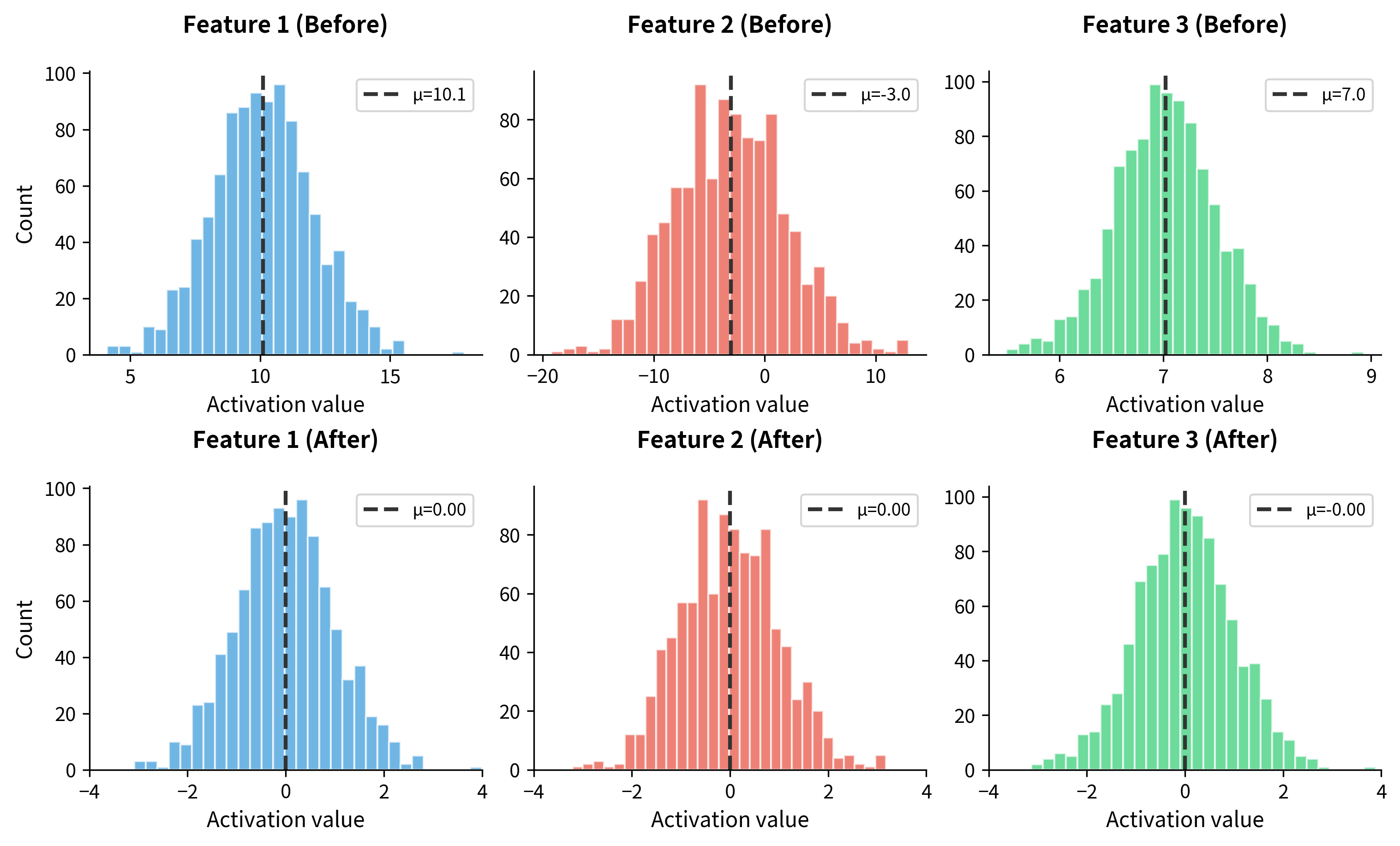
The visualization makes the effect immediately clear. Before normalization, each feature has a different center and spread, with Feature 1 centered around 10, Feature 2 around -3, and Feature 3 around 7. After normalization, all three features share the same standardized distribution, centered at zero with comparable spread. This consistency is what enables stable training.

We've just forced all activations to have zero mean and unit variance. But wait: what if the optimal representation for a particular layer actually needs activations centered around 3.7 with a spread of 0.5? By hardcoding zero mean and unit variance, we've potentially crippled the network's ability to learn the best representation.

This is where batch normalization gets clever. After normalizing, we apply a learnable affine transformation that can recover any mean and variance the network needs:

where:

• $y_i$: the final output of batch normalization for sample $i$
• $\gamma$: a learnable scale parameter (initialized to 1)
• $\hat{x}_i$: the normalized activation with zero mean and unit variance
• $\beta$: a learnable shift parameter (initialized to 0)

Think of $\gamma$ and $\beta$ as the network's way of saying "I understand you've normalized everything to standard form, but let me adjust it to what I actually need." The scale parameter $\gamma$ stretches or compresses the distribution, while the shift parameter $\beta$ moves it left or right along the number line.

Here's the beautiful part: if the network learns $\gamma = \sigma_\mathcal{B}$ and $\beta = \mu_\mathcal{B}$, it completely undoes the normalization, recovering the original activations. This means batch normalization can never hurt representational capacity. In the worst case, the network learns to bypass it entirely. In practice, the network finds some intermediate setting that benefits from the normalized optimization landscape while still representing the patterns it needs.

The crucial insight is what gets learned versus what gets computed. The mean and variance ($\mu_\mathcal{B}$, $\sigma^2_\mathcal{B}$) are computed from the batch data, not learned parameters. They stabilize the forward pass by keeping activations well-scaled. Meanwhile, $\gamma$ and $\beta$ are learned through backpropagation, giving the network control over the final representation. This separation decouples the mechanics of stable training from the semantics of learned features.

With custom parameters, the output mean equals $\beta$ and the standard deviation equals $|\gamma|$, as expected from the transformation $y = \gamma \hat{x} + \beta$ where $\hat{x}$ has zero mean and unit variance.

Let's visualize how different $\gamma$ and $\beta$ values transform the normalized distribution:

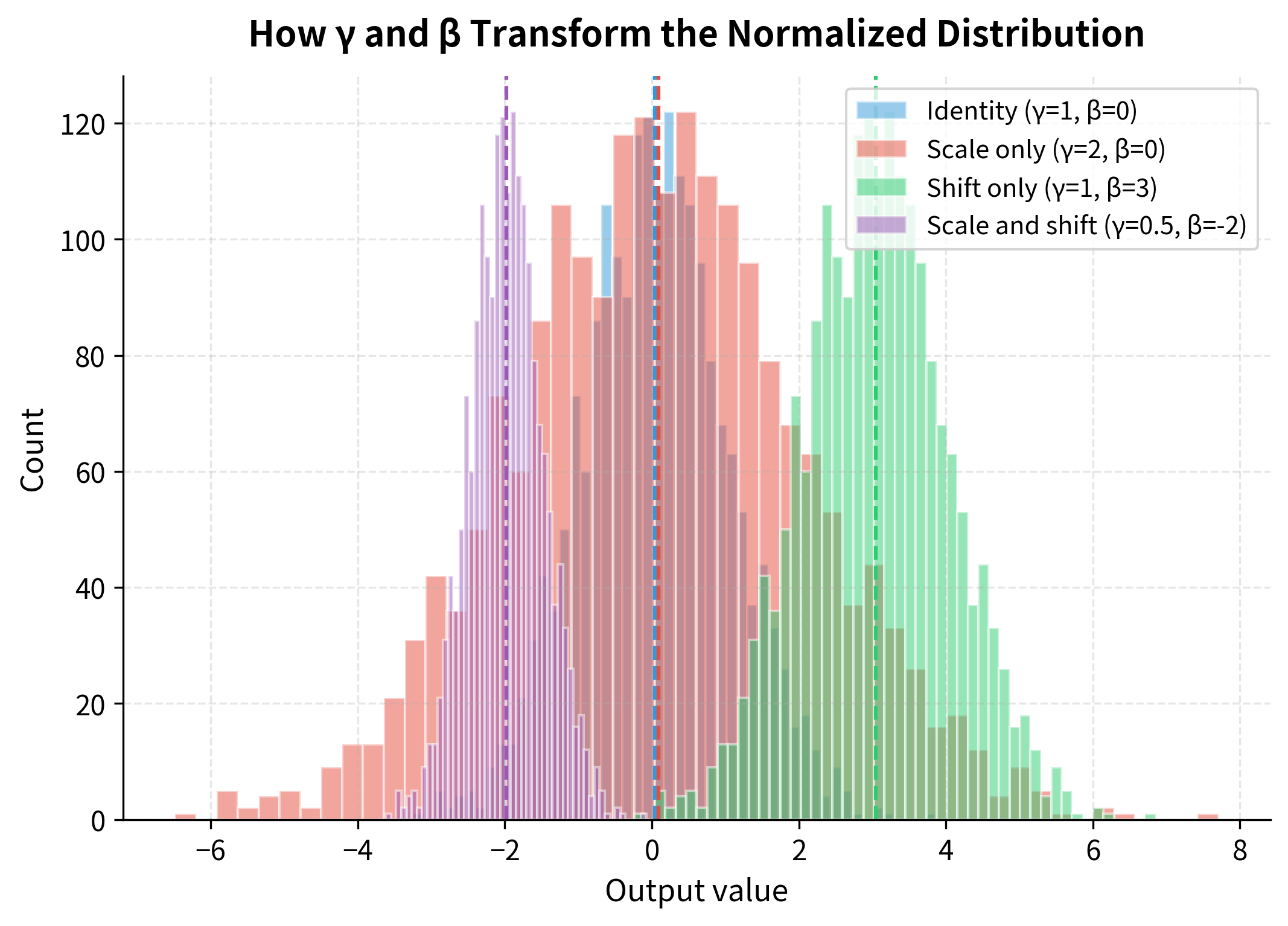
The visualization shows how the network can recover any distribution it needs. The blue distribution (identity) shows the standard normalized output. Scaling by $\gamma = 2$ (red) doubles the spread. Shifting by $\beta = 3$ (green) moves the center. Combining both (purple) demonstrates that the network can learn to place the distribution anywhere with any spread. This flexibility is crucial: batch normalization stabilizes training without constraining what the network can represent.

Batch normalization behaves differently during training and inference, which is a critical detail that often causes bugs.

During training, batch normalization uses the current mini-batch statistics ($\mu_\mathcal{B}$, $\sigma^2_\mathcal{B}$) for normalization. This introduces stochasticity since different batches have slightly different statistics, which acts as a regularizer.

During inference, using batch statistics is problematic. We might have a single sample (batch size 1), making batch statistics meaningless. We also want deterministic predictions. Instead, we use running averages of mean and variance accumulated during training. After each training batch, we update:

where:

• $\mu_{\text{running}}$: the exponential moving average of batch means, used at inference time
• $\sigma^2_{\text{running}}$: the exponential moving average of batch variances
• $\alpha$: the momentum coefficient (typically 0.9 or 0.99), controlling how much weight is given to the existing running average versus the new batch statistics
• $\mu_\mathcal{B}$, $\sigma^2_\mathcal{B}$: the mean and variance computed from the current mini-batch

These running statistics approximate the population statistics and are used for normalization at inference time.

Let's visualize how the running statistics evolve during training to see the convergence process:

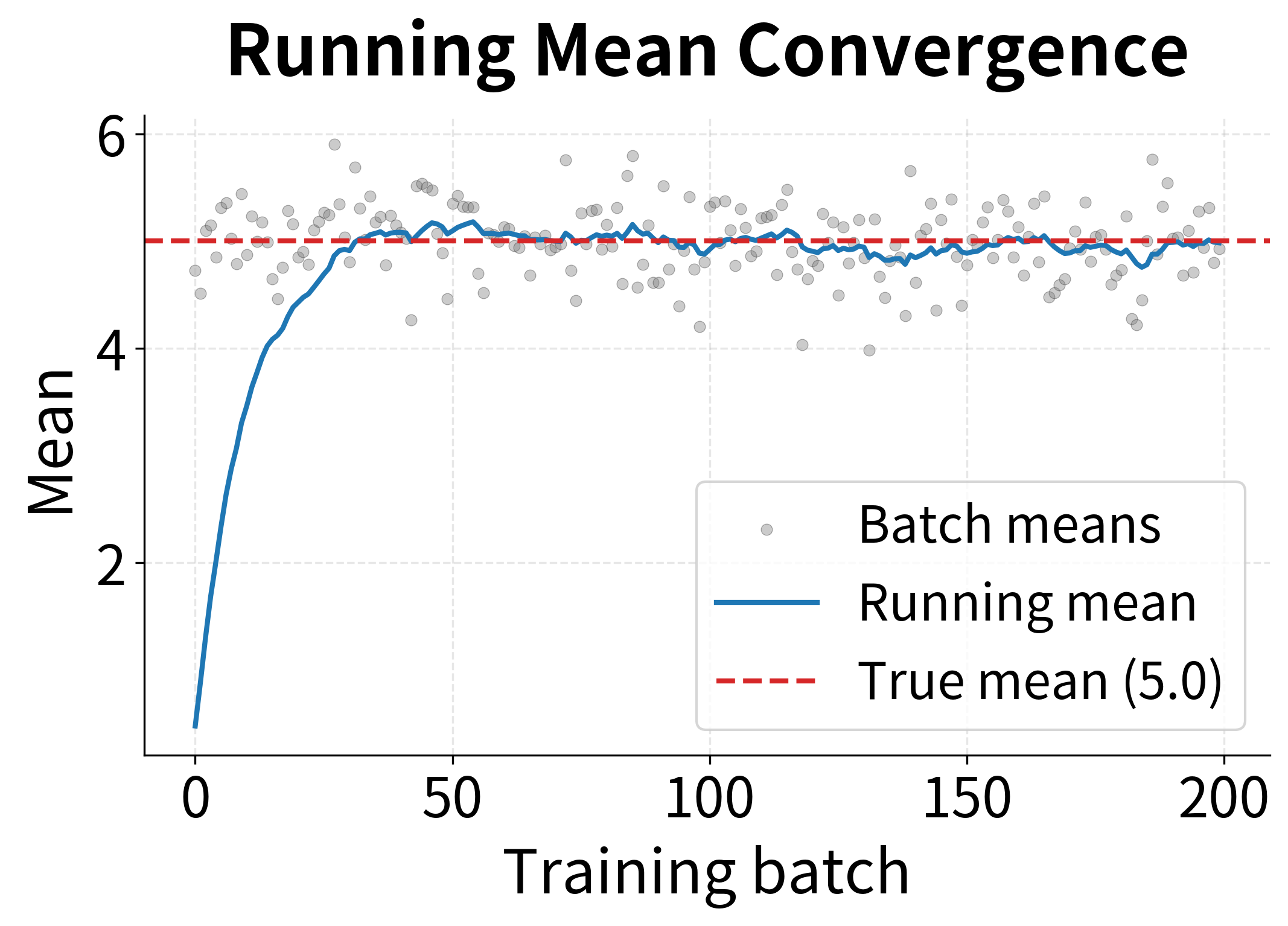
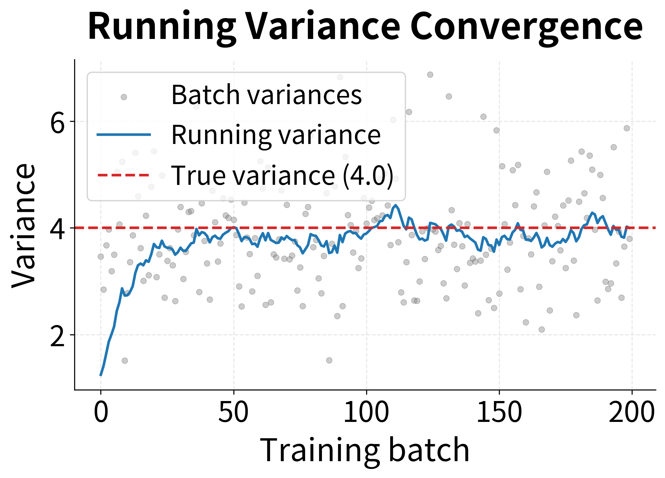
The visualization reveals an important property: individual batch statistics (gray dots) fluctuate considerably due to sampling noise, but the exponential moving average smooths out these fluctuations, converging steadily toward the true population values. This is why we use running statistics for inference rather than batch statistics. A single test sample would give meaningless batch statistics, but the running average provides stable, reliable normalization.

Understanding how gradients flow through batch normalization is essential for both implementation and debugging. The backward pass is more complex than the forward pass, and the reason reveals something fundamental about how batch normalization operates.

In a typical neural network layer, each input affects only its own output. The activation $x_1$ flows through the layer and contributes to $y_1$, independent of what $x_2$ or $x_3$ are doing. Batch normalization breaks this independence. When we compute the batch mean, every input contributes. When we compute the variance, every input contributes again. This means that changing $x_1$ affects not just $y_1$, but every output in the batch, because $x_1$ shifts the mean and variance that normalize everyone.

This interconnection makes the gradient computation more intricate. We can't just compute $\frac{\partial y_i}{\partial x_i}$ and call it a day. We need to account for how $x_i$ affects the batch statistics, and how those statistics affect all outputs. Let's work through this step by step.

Given the loss $L$ and the upstream gradient $\frac{\partial L}{\partial y}$, we need to compute gradients with respect to $\gamma$, $\beta$, and the input $x$.

Gradients for the learnable parameters. Since $y_i = \gamma \hat{x}_i + \beta$, the gradients follow directly from the chain rule:

where:

• $\frac{\partial L}{\partial y_i}$: the upstream gradient flowing back from the loss with respect to output $y_i$
• $\hat{x}_i$: the normalized activation, which acts as a scaling factor for the $\gamma$ gradient

The $\beta$ gradient is simply the sum of upstream gradients because $\beta$ shifts all outputs equally.

Gradient with respect to the normalized input. This requires applying the chain rule through the scale parameter:

Gradient with respect to variance. Here the derivation becomes more involved because the variance affects all normalized outputs. Recall that $\hat{x}_i = (x_i - \mu) / \sqrt{\sigma^2 + \epsilon}$, so the variance appears in the denominator:

The term $(\sigma^2 + \epsilon)^{-3/2}$ comes from differentiating $(\sigma^2 + \epsilon)^{-1/2}$ with respect to $\sigma^2$.

Gradient with respect to mean. The mean affects the normalized output both directly (in the numerator) and indirectly through the variance:

The first term captures the direct effect (the $-\mu$ in the numerator), while the second term captures how changing $\mu$ affects the variance calculation.

Gradient with respect to input. Finally, we combine all pathways through which $x_i$ affects the loss:

where:

• The first term: the direct effect of $x_i$ on its own normalized value $\hat{x}_i$
• The second term: the effect of $x_i$ on the batch variance (each input contributes to the variance)
• The third term: the effect of $x_i$ on the batch mean (each input contributes equally, hence the $\frac{1}{m}$ factor)

The key insight is that each input affects all outputs through the shared batch statistics. This creates dependencies that must be properly accounted for during backpropagation.

The analytical and numerical gradients match closely, confirming our backward pass implementation is correct. The small relative error is due to floating-point precision in the numerical approximation.

Where to place batch normalization in the network architecture has been debated since its introduction. The original paper proposed placing it before the activation function, but subsequent research and practice have explored alternatives.

Before activation (original proposal):

where $W$ is the weight matrix, $x$ is the input, $b$ is the bias, BN denotes batch normalization, and activation is the nonlinear function (e.g., ReLU). The reasoning: normalize the linear transformation's output before the nonlinearity, ensuring the activation receives well-conditioned inputs.

After activation (alternative):

Some practitioners find this works better for certain architectures. The intuition is that normalizing the activation's output directly controls what the next layer sees.

Without bias:

When using batch normalization before or after a linear layer, the bias term becomes redundant. The batch norm's $\beta$ parameter can learn any shift, so we simplify to:

Most frameworks use this optimization by default.

The placement choice often comes down to empirical performance on your specific task. Both approaches work well in practice, though the "before activation" pattern remains more common in modern architectures.

Let's see how batch normalization integrates into a complete training loop using PyTorch:

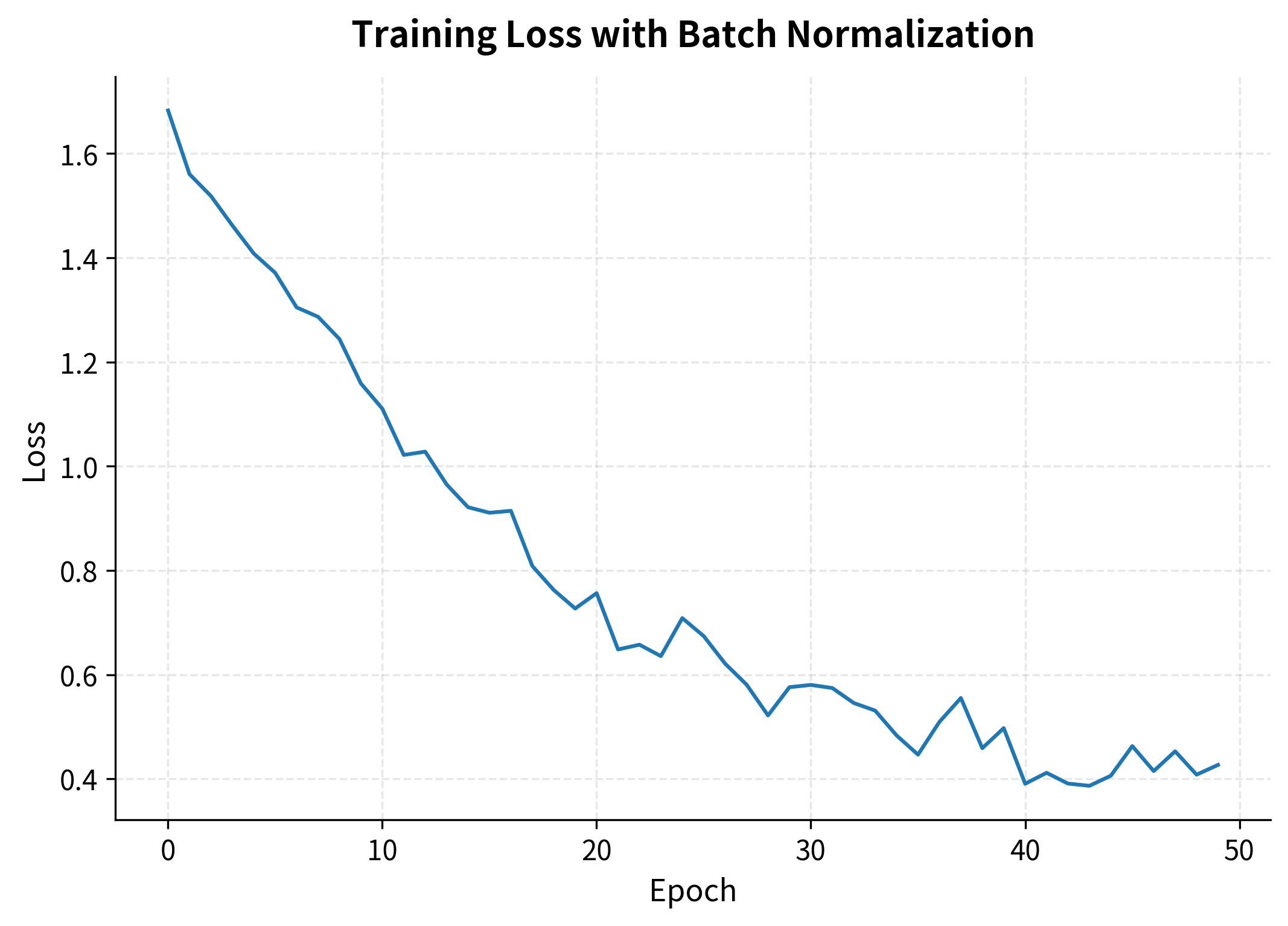
The training converges smoothly even with a relatively high learning rate of 0.01. Without batch normalization, the same network might require a much smaller learning rate or fail to converge at all.

The learned $\gamma$ values hover around 1 and $\beta$ values around 0, indicating the network hasn't needed to drastically rescale the normalized activations. The running statistics show the accumulated mean and variance from training.

To appreciate batch normalization's impact, let's compare identical networks with and without it:

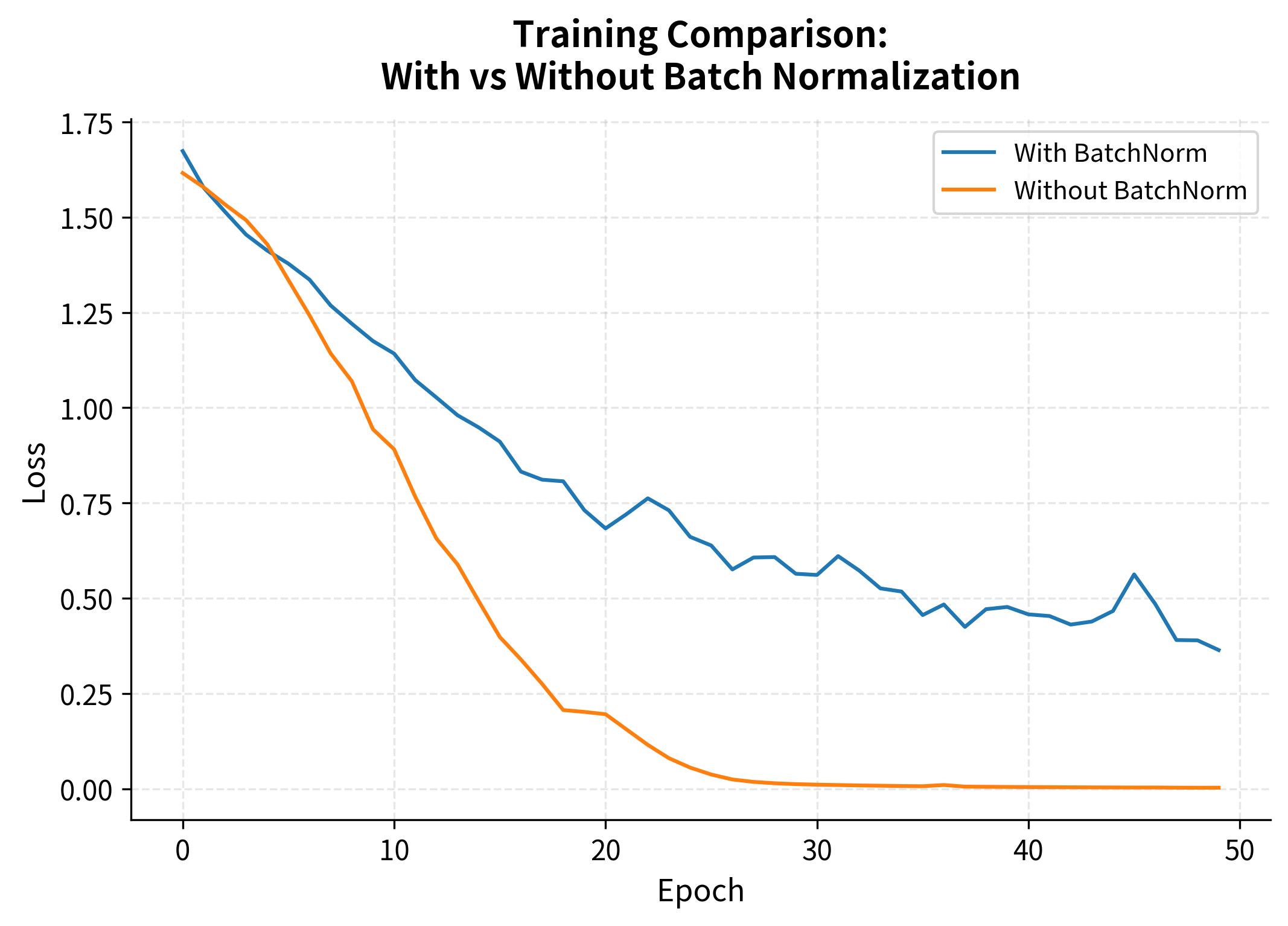
Both networks eventually converge, but the batch normalized version converges faster and more smoothly. The difference becomes more pronounced with deeper networks and higher learning rates.

Batch normalization transformed deep learning, but it comes with significant limitations that have motivated alternative normalization techniques.

The most fundamental limitation is batch size dependency. Batch normalization requires sufficiently large batches to compute meaningful statistics. With very small batches (fewer than 8-16 samples), the batch mean and variance become noisy estimates of the population statistics, destabilizing training. This is particularly problematic in domains like object detection and 3D medical imaging, where memory constraints force small batch sizes, or in reinforcement learning, where samples within a batch may be highly correlated. In these settings, practitioners either use alternative normalizations (Layer Norm, Group Norm, Instance Norm) or accumulate gradient updates across multiple forward passes before applying them.

The training/inference discrepancy is another source of subtle bugs. During training, batch statistics introduce stochasticity that can differ significantly from the running statistics used at inference. If the data distribution at test time differs from training, the running statistics may be inappropriate. A common symptom is a model that performs well during training but poorly at inference, often traced back to batch normalization layers that haven't accumulated representative statistics. Always ensure you process enough training data for running statistics to stabilize, and call model.eval() during inference.

Batch normalization also introduces dependencies between samples in a batch. Each sample's normalized value depends on all other samples through the shared mean and variance. This breaks the independence assumption used in some theoretical analyses and can cause issues when the batch composition is non-random (for example, when all samples in a batch come from the same class). In sequence models, this dependency is particularly problematic, which is why Transformers use Layer Normalization instead.

Finally, batch normalization adds computational overhead. Computing statistics, normalizing, and applying learnable parameters adds operations during both forward and backward passes. The overhead is typically small compared to the benefits, but it's not negligible in latency-sensitive applications.

Despite these limitations, batch normalization remains extremely popular because it works well for most feedforward and convolutional networks with reasonable batch sizes. Understanding when it's appropriate, and when to use alternatives, is a key practical skill.

When using batch normalization in PyTorch or implementing it from scratch, the following parameters control its behavior:

• num_features: The number of features (channels) to normalize. Must match the size of the feature dimension in the input tensor. For a fully connected layer with 128 outputs, use BatchNorm1d(128).

• eps (default: $10^{-5}$): A small constant added to the variance for numerical stability. Prevents division by zero when variance is very small. Rarely needs adjustment.

• momentum (default: 0.1 in PyTorch): Controls the running statistics update rate. PyTorch uses the convention $(1 - \text{momentum}) \cdot \text{running\_stat} + \text{momentum} \cdot \text{batch\_stat}$, so higher values mean faster adaptation to recent batches. Values between 0.01 and 0.1 work well for most cases.

• affine (default: True): Whether to include learnable $\gamma$ and $\beta$ parameters. Setting to False removes the scale and shift, which is rarely useful but can reduce parameters in specific architectures.

• track_running_stats (default: True): Whether to maintain running mean and variance for inference. Set to False only if you want batch statistics at inference time (unusual).

The most common configuration uses default values with bias=False on the preceding linear layer, since the batch norm's $\beta$ parameter subsumes the bias term.

Batch normalization addresses internal covariate shift by normalizing layer inputs using mini-batch statistics. For each feature, it computes the batch mean and variance, normalizes to zero mean and unit variance, then applies learnable scale ($\gamma$) and shift ($\beta$) parameters. This decoupling of activation statistics from learned representations stabilizes training and enables higher learning rates.

The key concepts covered in this chapter:

• Internal covariate shift: The shifting input distributions that make deep network training difficult
• Batch statistics: Mean and variance computed per feature across the mini-batch
• Learnable parameters: $\gamma$ and $\beta$ that preserve representational capacity
• Training vs inference: Batch statistics during training, running averages during inference
• Gradient flow: The backward pass accounts for how each input affects batch statistics
• Placement: Usually before activation, often without bias in preceding linear layers
• Limitations: Batch size dependency, training/inference discrepancy, sample dependencies

Batch normalization was a breakthrough that enabled training of much deeper networks. While alternatives like Layer Normalization have become preferred for certain architectures (particularly Transformers), understanding batch normalization remains essential, as it forms the foundation for the entire family of normalization techniques used in modern deep learning.

Ready to test your understanding? Take this quick quiz to reinforce what you've learned about batch normalization.