InteractiveCo-occurrence Matrices: Building Word Representations from Context

Co-occurrence MatricesLink Copied

The distributional hypothesis tells us that words appearing in similar contexts have similar meanings. But how do we actually capture and quantify these contextual patterns? The answer lies in co-occurrence matrices, the foundational data structures that transform raw text into numerical representations of word relationships.

In this chapter, you'll learn how to construct matrices that encode which words appear near which other words, and how different design choices affect what patterns these matrices capture. These matrices serve as the raw material for more sophisticated techniques like PMI weighting and dimensionality reduction, which we'll explore in subsequent chapters.

The Core Idea: Counting ContextLink Copied

At its heart, a co-occurrence matrix is simply a way to count how often words appear together. Consider a small corpus:

"The cat sat on the mat. The dog sat on the rug."

If we want to know what contexts the word "sat" appears in, we look at its neighbors. Both "cat" and "dog" appear before "sat," while "on" appears after it. By systematically counting these patterns across a large corpus, we build a picture of each word's distributional profile.

This approach is simple. We don't need linguistic rules, parse trees, or semantic annotations. We just count. And from these counts, meaningful patterns emerge.

Two Types of Co-occurrence MatricesLink Copied

There are two main flavors of co-occurrence matrices, each capturing different aspects of word relationships.

Word-Word Co-occurrence MatricesLink Copied

A word-word matrix counts how often pairs of words appear near each other within a local context window. If your vocabulary has $V$ words, you get a $V \times V$ matrix.

The key parameter is the context window size, which defines "near." A window of size 2 means we count words that appear within 2 positions to the left or right of the target word.

For our example sentence "The cat sat on the mat," with a window size of 2, the word "sat" has context words {the, cat, on, the}. We increment the co-occurrence counts for each of these pairs.

Word-Document Co-occurrence MatricesLink Copied

A word-document matrix (also called a term-document matrix) counts how often each word appears in each document. If you have $V$ vocabulary words and $D$ documents, you get a $V \times D$ matrix.

This representation is widely used in information retrieval and topic modeling. Documents with similar word distributions are likely about similar topics. Latent Semantic Analysis (LSA) applies SVD to exactly this type of matrix.

For this chapter, we'll focus primarily on word-word matrices, as they capture the fine-grained local context that's most relevant for learning word meanings.

Building a Word-Word Co-occurrence MatrixLink Copied

Let's build a co-occurrence matrix from scratch. We'll start with a small corpus to see exactly what's happening, then scale up to real text.

Our vocabulary contains 8 unique words. Each word gets a unique integer index that we'll use to address rows and columns in our matrix.

Now let's build the co-occurrence matrix with a context window of size 1, meaning we only count immediately adjacent words.

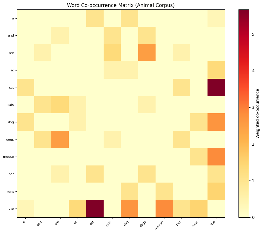
Each cell shows how many times the row word appeared adjacent to the column word. Notice that "the" co-occurs frequently with many words since it's a common function word. Meanwhile, "cat" and "dog" both co-occur with "the," "sat," and "chased," reflecting their similar syntactic roles.

Let's visualize this matrix to see the patterns more clearly.

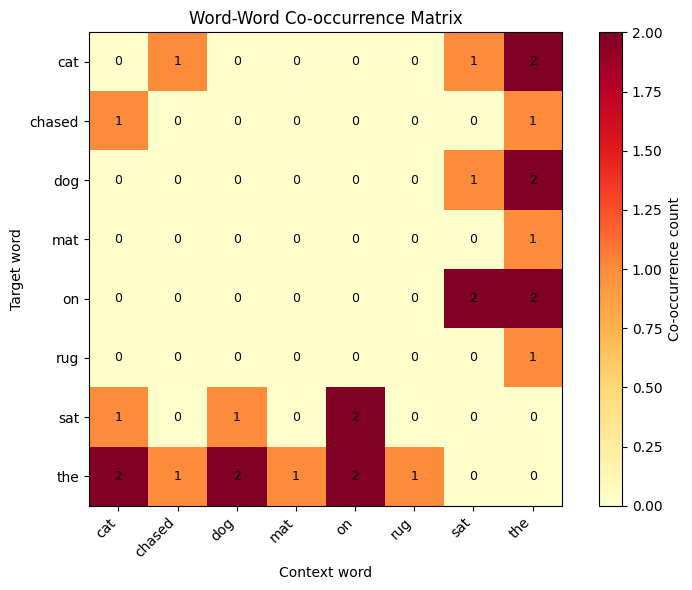
The heatmap reveals the structure of our tiny corpus. The bright row and column for "the" shows it co-occurs with almost everything, which is typical for function words. Content words like "cat," "dog," "mat," and "rug" show sparser patterns that reflect their actual usage.

Context Window Size EffectsLink Copied

The window size parameter has a major effect on what relationships your matrix captures. Let's explore this with a larger, more realistic corpus.

Now let's compare matrices built with different window sizes.

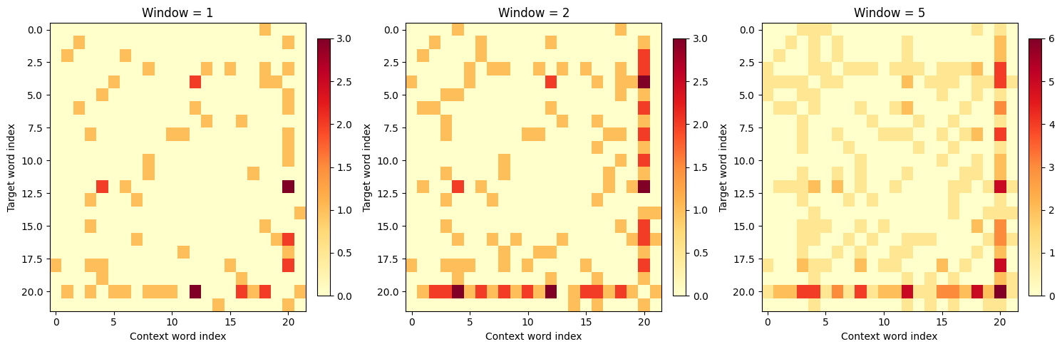
The visual difference is clear. With window size 1, the matrix is sparse, capturing only immediate neighbors. As we increase the window, more cells fill in, and the matrix becomes denser. By window size 5, nearly every word pair has some co-occurrence.

Let's quantify this sparsity difference.

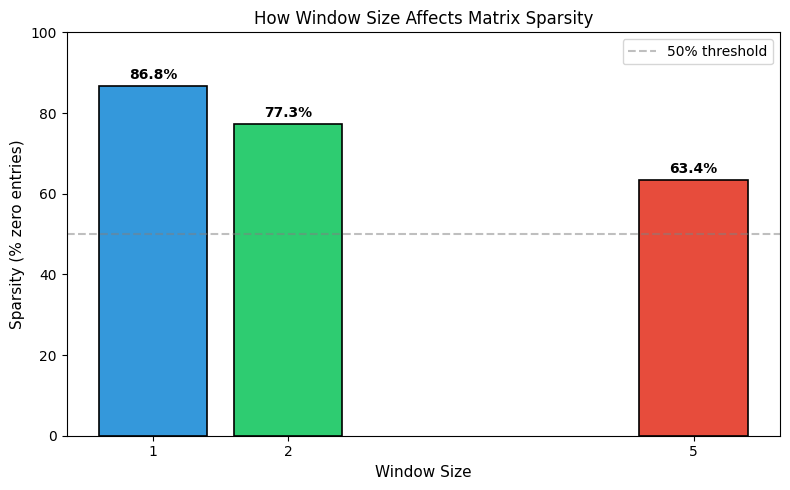
The bar chart makes the trade-off clear: window size 1 produces an extremely sparse matrix (mostly zeros), while window size 5 fills in substantially more entries.

The choice of window size depends on your downstream task. For syntax-focused applications like part-of-speech tagging, smaller windows work better. For semantic similarity and topic modeling, larger windows capture more meaningful relationships.

Weighting by DistanceLink Copied

Not all context positions are equally informative. A word immediately adjacent to your target is more relevant than one five positions away. Distance weighting addresses this by giving closer words higher counts.

The most common approach is harmonic weighting, where a context word at distance $d$ contributes $\frac{1}{d}$ instead of 1:

where:

• $d$: the distance (in word positions) between the target word and context word, always a positive integer

The following plot shows how harmonic weights decay with distance, compared to uniform weighting where all positions contribute equally.

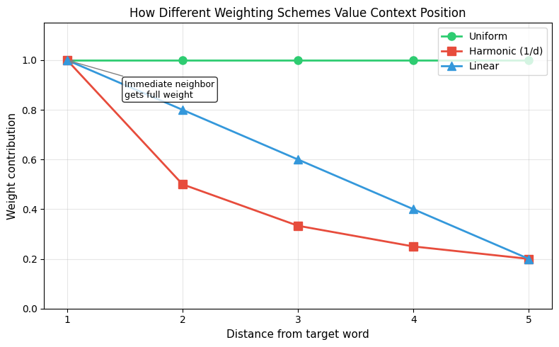
This makes sense: a word right next to your target is highly relevant, while one five positions away provides weaker evidence of association.

Let's implement this.

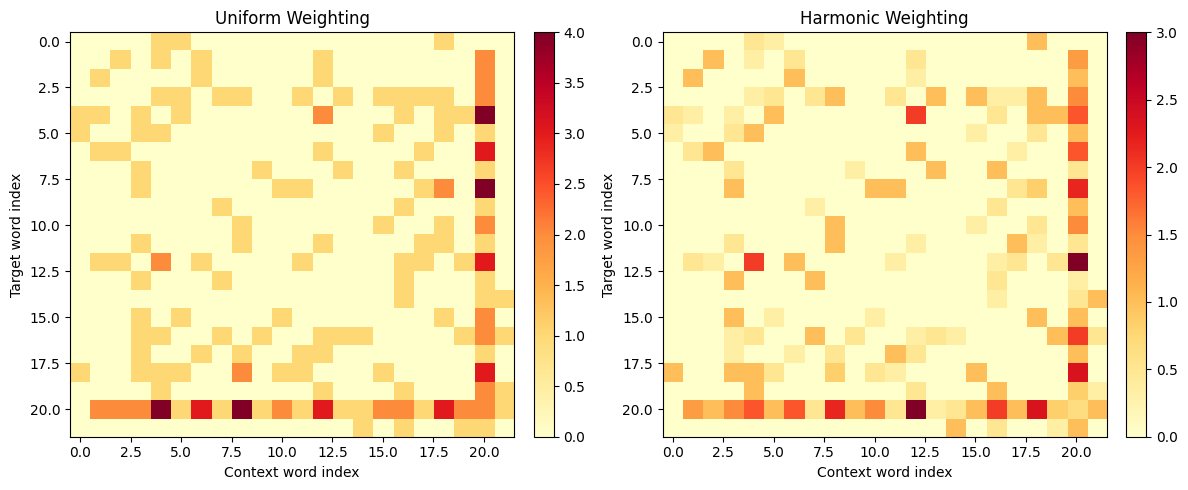
The harmonic-weighted matrix has lower overall values because distant context words contribute fractional amounts. This weighting scheme was popularized by GloVe and has become standard practice in modern word embedding methods.

Symmetric vs Directional ContextsLink Copied

So far, we've treated left and right context symmetrically. If "cat" appears before "sat," we count it the same as if it appeared after. But in some cases, you might want to distinguish direction.

Symmetric contexts treat position as irrelevant. This is the standard approach and what we've been doing. The resulting matrix is symmetric: $M_{ij} = M_{ji}$.

Directional contexts distinguish left from right. You might have separate matrices for "words that appear before" and "words that appear after," or double your vocabulary to include position markers.

Directional contexts can capture asymmetric relationships. For instance, in English, determiners almost always appear to the left of nouns. A directional matrix would capture this pattern, while a symmetric matrix would lose it.

Matrix Sparsity and StorageLink Copied

Real-world co-occurrence matrices are enormous and extremely sparse. With a vocabulary of 100,000 words, you'd have a $100,000 \times 100,000 = 10^{10}$ cell matrix. Most of these cells will be zero since any given word only co-occurs with a tiny fraction of the vocabulary.

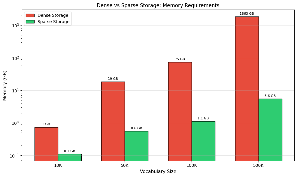
The numbers tell the story. A dense 100K vocabulary matrix would require 74 GB of memory. The same information stored sparsely needs only about 1 GB. This is why sparse matrix formats are necessary for practical applications.

Let's see how to use sparse matrices in practice with scipy.

For our tiny example, the overhead of sparse storage actually makes it larger. But as matrices grow, sparse storage becomes necessary.

Efficient Construction at ScaleLink Copied

When processing large corpora, naive implementations become prohibitively slow. Here are key optimizations for building co-occurrence matrices efficiently.

Streaming ConstructionLink Copied

Instead of loading the entire corpus into memory, process it in chunks.

Vocabulary FilteringLink Copied

In practice, you'll want to filter the vocabulary to exclude very rare words (which have unreliable statistics) and very common words (which dominate the matrix without adding much information).

The word "the" appears in every sentence, so it exceeds our 90% document frequency threshold and gets filtered out. This is a simple form of stopword removal based purely on statistics.

From Counts to SimilarityLink Copied

Once you have a co-occurrence matrix, you can compute word similarity by comparing rows. Words with similar co-occurrence patterns (those appearing in similar contexts) should have similar meanings.

The simplest approach is cosine similarity between row vectors.

To understand why certain words are similar, we can visualize their distributional profiles (the row vectors from the co-occurrence matrix).

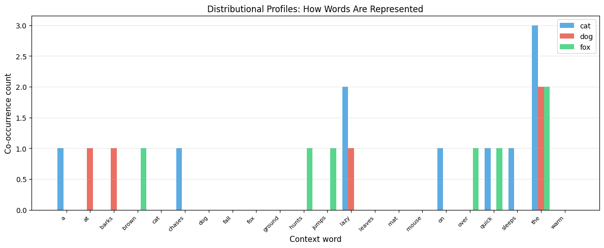
The bar chart reveals why "cat" and "dog" are similar: they share high co-occurrence with the same context words (like "the" and "lazy"). "Fox" has a different profile, co-occurring with different words.

Even with our tiny corpus, the similarity captures some meaningful patterns. "Cat" and "dog" are similar because they both appear with "the," "sat," and "chases/barks." The results would be much more meaningful with a larger corpus.

A Real-World ExampleLink Copied

Let's apply everything we've learned to a real text corpus. We'll use a subset of text to keep things manageable while demonstrating realistic patterns.

Now let's find similar words in this more meaningful corpus.

We can visualize the full similarity structure by computing pairwise cosine similarities between all words.

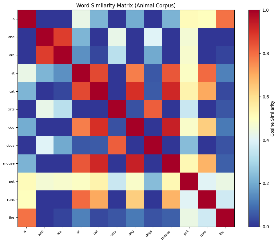
The similarity heatmap reveals the structure learned from co-occurrence patterns. The diagonal is always 1.0 (perfect self-similarity), and off-diagonal bright cells show which words have similar distributional profiles.

The results reflect the corpus content. "Cat" is similar to "the" (they co-occur frequently), "dog" (both are pets), and other contextually related words. With a larger corpus, these patterns become more reliable and meaningful.

Limitations and What Comes NextLink Copied

Raw co-occurrence counts have limitations that motivate the techniques in upcoming chapters.

Frequency bias: Common words dominate the matrix. "The" appears everywhere, so it has high co-occurrence with everything, even though this tells us little about word meaning. We need weighting schemes like PMI to address this.

Dimensionality: Even with a modest 50,000-word vocabulary, you have 50,000-dimensional vectors. This is computationally expensive and prone to noise. Dimensionality reduction techniques like SVD compress these vectors while preserving meaningful structure.

Sparsity: Most word pairs never co-occur, leaving the matrix mostly zeros. This sparsity makes similarity computations unreliable for rare words. Dense embeddings learned through neural methods address this limitation.

Despite these limitations, co-occurrence matrices remain the foundation of distributional semantics. Understanding how they work, what design choices matter, and what patterns they capture prepares you for the more sophisticated techniques built on top of them.

SummaryLink Copied

In this chapter, you learned how to transform raw text into numerical representations through co-occurrence matrices.

Key concepts:

• Word-word matrices count how often pairs of words appear near each other, capturing local context patterns
• Context window size controls what relationships you capture: small windows for syntax, large windows for semantics
• Distance weighting gives more importance to closer context words, typically using harmonic weights ($\frac{1}{d}$)
• Symmetric vs directional contexts trade off simplicity against capturing word order information
• Sparse storage is necessary for real-world vocabulary sizes, reducing memory by orders of magnitude

Practical considerations:

• Filter vocabulary by frequency to remove noise from rare words and uninformative function words
• Use streaming construction for large corpora that don't fit in memory
• Cosine similarity between row vectors gives a simple word similarity measure

The raw counts in co-occurrence matrices are just the starting point. In the next chapter, we'll see how Pointwise Mutual Information transforms these counts into more meaningful association scores that better capture word relationships.

Key ParametersLink Copied

When building co-occurrence matrices, these parameters have the greatest impact on the resulting representations:

Choosing window size: Start with 2-5 for general-purpose representations. Use smaller windows (1-2) if syntactic patterns matter, larger windows (5-10) for topic-level similarity.

Choosing weighting: Harmonic weighting is the default choice for most applications. It's used by GloVe and produces more balanced representations than uniform weighting.

Vocabulary filtering: For large corpora, use min_count=5 and max_freq=0.7 as starting points. Adjust based on corpus size and downstream task requirements.

QuizLink Copied

Ready to test your understanding? Take this quick quiz to reinforce what you've learned about co-occurrence matrices and distributional semantics.