Perplexity: The Standard Metric for Evaluating Language Models

Michael Brenndoerfer

Learn how perplexity measures language model quality through cross-entropy and information theory. Understand the branching factor interpretation, implement perplexity for n-gram models, and discover when perplexity predicts downstream performance.

Part of Language AI Handbook

This article is part of the free-to-read Language AI Handbook

Reading Level

Choose your expertise level to adjust how many terms are explained. Beginners see more tooltips, experts see fewer to maintain reading flow. Hover over underlined terms for instant definitions.

PerplexityLink Copied

You've built an n-gram language model and applied smoothing techniques. Now comes the critical question: how good is your model? Perplexity provides the answer. It's the standard metric for evaluating language models, used everywhere from academic papers to production systems. Understanding perplexity shows not just how to measure model quality, but what it means for a model to "understand" language.

This chapter develops perplexity from first principles. We'll derive it from information theory, connect it to intuitive concepts like "branching factor," implement it from scratch, and explore both its power and its limitations.

The Evaluation ProblemLink Copied

Consider two language models trained on the same corpus. Model A assigns $P(\text{"the cat sat on the mat"}) = 0.001$ . Model B assigns $P(\text{"the cat sat on the mat"}) = 0.0001$ . Which model is better?

At first glance, Model A seems superior because it assigns higher probability to a grammatical sentence. But this comparison is misleading. Model A might assign high probability to everything, including nonsense like "mat the on sat cat the." Model B might be more discriminating, reserving high probability for truly likely sequences.

We need a metric that rewards models for assigning high probability to actual language while penalizing them for wasting probability mass on unlikely sequences. Perplexity does exactly this by measuring how well a model predicts held-out test data.

Held-Out Evaluation

The practice of evaluating a model on data it wasn't trained on. This tests whether the model learned generalizable patterns rather than memorizing the training data. The held-out data is called the test set or evaluation set.

Cross-Entropy: The FoundationLink Copied

To measure how well a language model predicts text, we need a principled way to quantify "prediction quality." This is where information theory provides the perfect framework. The key insight is that prediction and compression are two sides of the same coin: if you can predict what comes next, you can compress it efficiently. Cross-entropy formalizes this connection, and perplexity translates it into an intuitive scale.

Let's build up to perplexity step by step, starting with the most fundamental question: how do we measure uncertainty?

Entropy: Quantifying UncertaintyLink Copied

Imagine you're playing a word-guessing game. Your friend thinks of a word, and you have to guess it using only yes/no questions. How many questions do you need?

The answer depends on how predictable the word is. If your friend always picks from {"cat", "dog"} with equal probability, you need exactly one question ("Is it cat?"). But if they pick from a thousand equally likely words, you need about 10 questions (since $2^{10} = 1024$ ). This number of questions is exactly what entropy measures.

For a probability distribution $P$ over a vocabulary $V$ , entropy is:

H(P) = -\sum_{w \in V} P(w) \log_2 P(w)

where:

$H(P)$ : entropy of distribution $P$ (measured in bits when using $\log_2$ )
$P(w)$ : probability of word $w$
The sum runs over all words in the vocabulary

The formula might look abstract, but it captures a clear intuition: each word contributes $-\log_2 P(w)$ bits (called the "surprisal" or "information content" of that word), weighted by how often it occurs. Rare words contribute more bits because they're more surprising, while common words contribute fewer.

Let's see this in action with a simple two-word vocabulary:

In[2]:

import numpy as np

def entropy(probs):
    """Calculate entropy of a probability distribution."""
    # Filter out zero probabilities to avoid log(0)
    probs = np.array([p for p in probs if p > 0])
    return -np.sum(probs * np.log2(probs))

# Different probability distributions over two words
distributions = [
    ([0.5, 0.5], "Equal probability"),
    ([0.9, 0.1], "Skewed (90/10)"),
    ([0.99, 0.01], "Very skewed (99/1)"),
    ([1.0, 0.0], "Certain"),
]

import numpy as np

def entropy(probs):
    """Calculate entropy of a probability distribution."""
    # Filter out zero probabilities to avoid log(0)
    probs = np.array([p for p in probs if p > 0])
    return -np.sum(probs * np.log2(probs))

# Different probability distributions over two words
distributions = [
    ([0.5, 0.5], "Equal probability"),
    ([0.9, 0.1], "Skewed (90/10)"),
    ([0.99, 0.01], "Very skewed (99/1)"),
    ([1.0, 0.0], "Certain"),
]

Out[3]:

Entropy for different distributions over {cat, dog}:
--------------------------------------------------
Equal probability         H = 1.0000 bits
Skewed (90/10)            H = 0.4690 bits
Very skewed (99/1)        H = 0.0808 bits
Certain                   H = -0.0000 bits

Notice the pattern: when both words are equally likely, entropy is maximal at 1 bit. You need one yes/no question. As one word dominates, entropy drops because the outcome becomes more predictable. When the outcome is certain, entropy is zero: no questions needed, no uncertainty remains.

Out[4]:

Visualization

Line plot showing entropy on y-axis versus probability of first outcome on x-axis, forming an inverted U shape with peak at 0.5. — Entropy as a function of probability distribution skew. When one outcome dominates (probability near 0 or 1), entropy approaches zero because the result is predictable. Maximum entropy occurs at equal probabilities (p=0.5), where uncertainty is highest.

This gives us our first key insight: entropy measures the inherent unpredictability of a distribution. A good language model should have low entropy on real text because it can predict what comes next.

Cross-Entropy: Measuring Model MismatchLink Copied

Entropy tells us about the true distribution, but we don't have access to that. We only have our model's predictions. This is where cross-entropy enters the picture.

Cross-entropy asks: "If the true distribution is $P$ , but we use model $Q$ to make predictions, how many bits do we need on average?" The answer is always at least as many as entropy, and usually more, because our model isn't perfect.

H(P, Q) = -\sum_{w \in V} P(w) \log_2 Q(w)

where:

$H(P, Q)$ : cross-entropy of $P$ relative to $Q$
$P(w)$ : true probability of word $w$ (from the data)
$Q(w)$ : model's predicted probability of word $w$

The key relationship is: $H(P, Q) \geq H(P)$ . Cross-entropy is always at least as large as entropy. The gap between them, called KL divergence, measures exactly how much our model's predictions differ from reality.

Think of it this way:

Entropy $H(P)$ : the minimum bits needed with a perfect model
Cross-entropy $H(P, Q)$ : the bits needed with our actual model $Q$
KL divergence $H(P, Q) - H(P)$ : the "cost" of using an imperfect model

Out[5]:

Visualization

Stacked bar chart showing how cross-entropy decomposes into entropy plus KL divergence for different model qualities. — Decomposition of cross-entropy into entropy and KL divergence. The entropy (blue) represents the inherent uncertainty in the data, the minimum bits needed with a perfect model. The KL divergence (orange) represents the additional cost of using an imperfect model. Better models have smaller KL divergence.

In practice, we don't know the true distribution $P$ . Instead, we approximate it using the empirical distribution from our test data. If word $w$ appears $C(w)$ times in a test corpus of $N$ words, we estimate:

\hat{P}(w) = \frac{C(w)}{N}

This leads to a simple practical formula:

H(\hat{P}, Q) = -\frac{1}{N} \sum_{i=1}^{N} \log_2 Q(w_i)

In words: cross-entropy is the average negative log probability that our model assigns to each word in the test corpus. Lower is better because it means the model assigned higher probabilities to the words that actually appeared.

Let's compute this for a simple unigram model:

In[6]:

def cross_entropy(test_tokens, model_probs):
    """
    Calculate cross-entropy of a model on test data.
    
    Args:
        test_tokens: List of tokens from test corpus
        model_probs: Function that returns P(token | context)
    """
    log_prob_sum = 0.0
    count = 0
    
    for i, token in enumerate(test_tokens):
        prob = model_probs(token, i, test_tokens)
        if prob > 0:
            log_prob_sum += np.log2(prob)
            count += 1
        else:
            # Handle zero probability (model assigns impossible)
            return float('inf')
    
    return -log_prob_sum / count

# Simple unigram model for demonstration
train_corpus = """
the cat sat on the mat
the dog sat on the rug
the cat chased the dog
the dog chased the cat
""".lower().split()

from collections import Counter
word_counts = Counter(train_corpus)
total_words = len(train_corpus)

def unigram_prob(token, position, tokens):
    """Return unigram probability P(token)."""
    count = word_counts.get(token, 0)
    # Add-1 smoothing to handle unseen words
    vocab_size = len(word_counts) + 1  # +1 for unknown
    return (count + 1) / (total_words + vocab_size)

# Test on held-out data
test_corpus = "the cat sat on the rug".split()

def cross_entropy(test_tokens, model_probs):
    """
    Calculate cross-entropy of a model on test data.
    
    Args:
        test_tokens: List of tokens from test corpus
        model_probs: Function that returns P(token | context)
    """
    log_prob_sum = 0.0
    count = 0
    
    for i, token in enumerate(test_tokens):
        prob = model_probs(token, i, test_tokens)
        if prob > 0:
            log_prob_sum += np.log2(prob)
            count += 1
        else:
            # Handle zero probability (model assigns impossible)
            return float('inf')
    
    return -log_prob_sum / count

# Simple unigram model for demonstration
train_corpus = """
the cat sat on the mat
the dog sat on the rug
the cat chased the dog
the dog chased the cat
""".lower().split()

from collections import Counter
word_counts = Counter(train_corpus)
total_words = len(train_corpus)

def unigram_prob(token, position, tokens):
    """Return unigram probability P(token)."""
    count = word_counts.get(token, 0)
    # Add-1 smoothing to handle unseen words
    vocab_size = len(word_counts) + 1  # +1 for unknown
    return (count + 1) / (total_words + vocab_size)

# Test on held-out data
test_corpus = "the cat sat on the rug".split()

Out[7]:

Test corpus: the cat sat on the rug
Cross-entropy: 2.8692 bits per word

The cross-entropy tells us how many bits on average our model needs to encode each word. This number has a concrete interpretation: if we used our model's probabilities to design a compression scheme, each word would require about this many bits on average.

From Cross-Entropy to PerplexityLink Copied

Cross-entropy is useful, but "2.7 bits per word" doesn't immediately convey how good a model is. Is that good? Bad? It depends on the vocabulary size and the inherent predictability of the text.

Perplexity solves this by converting bits back to a count, specifically the number of equally likely choices. The transformation is simple:

\text{PP}(W) = 2^{H(P, Q)}

where:

$\text{PP}(W)$ : perplexity of the model on word sequence $W$
$H(P, Q)$ : cross-entropy between the true distribution $P$ and model distribution $Q$

Why raise 2 to the power of cross-entropy? Because entropy measures bits, and each bit doubles the number of possibilities. A cross-entropy of 3 bits means $2^3 = 8$ equally likely choices; 10 bits means $2^{10} = 1024$ choices.

Expanding this using our practical cross-entropy formula:

\text{PP}(W) = 2^{-\frac{1}{N} \sum_{i=1}^{N} \log_2 Q(w_i)}

where:

$N$ : total number of words in the test sequence
$w_i$ : the $i$ -th word in the sequence
$Q(w_i)$ : model's probability for word $w_i$ (given its context)

Using properties of logarithms, we can rewrite this as:

\text{PP}(W) = \left( \prod_{i=1}^{N} Q(w_i) \right)^{-\frac{1}{N}}

This shows that perplexity is the geometric mean of the inverse probabilities. Equivalently:

\text{PP}(W) = \frac{1}{\sqrt[N]{\prod_{i=1}^{N} Q(w_i)}}

The geometric mean matters here. Unlike the arithmetic mean, it's sensitive to very small probabilities. A single word with near-zero probability will dramatically increase perplexity. This is exactly what we want: a good language model shouldn't assign tiny probabilities to words that actually occur.

Perplexity

The perplexity of a language model on a test set is the inverse probability of the test set, normalized by the number of words. It can be interpreted as the weighted average number of choices the model faces at each step. Lower perplexity means the model is less "perplexed" by the test data.

For language models that condition on context (like n-gram models), we use conditional probabilities:

\text{PP}(W) = \sqrt[N]{\prod_{i=1}^{N} \frac{1}{P(w_i | w_1, \ldots, w_{i-1})}}

where $P(w_i | w_1, \ldots, w_{i-1})$ is the probability of word $w_i$ given all preceding words.

In practice, we work with log probabilities to avoid numerical underflow (multiplying many small probabilities quickly approaches zero):

\text{PP}(W) = 2^{-\frac{1}{N} \sum_{i=1}^{N} \log_2 P(w_i | w_1, \ldots, w_{i-1})}

In[8]:

def perplexity(test_tokens, model_log_prob):
    """
    Calculate perplexity of a model on test data.
    
    Args:
        test_tokens: List of tokens from test corpus
        model_log_prob: Function returning log2 P(token | context)
    """
    log_prob_sum = 0.0
    count = 0
    
    for i, token in enumerate(test_tokens):
        log_p = model_log_prob(token, i, test_tokens)
        if log_p == float('-inf'):
            return float('inf')  # Zero probability encountered
        log_prob_sum += log_p
        count += 1
    
    cross_ent = -log_prob_sum / count
    return 2 ** cross_ent

def unigram_log_prob(token, position, tokens):
    """Return log2 P(token) for unigram model with smoothing."""
    count = word_counts.get(token, 0)
    vocab_size = len(word_counts) + 1
    prob = (count + 1) / (total_words + vocab_size)
    return np.log2(prob)

def perplexity(test_tokens, model_log_prob):
    """
    Calculate perplexity of a model on test data.
    
    Args:
        test_tokens: List of tokens from test corpus
        model_log_prob: Function returning log2 P(token | context)
    """
    log_prob_sum = 0.0
    count = 0
    
    for i, token in enumerate(test_tokens):
        log_p = model_log_prob(token, i, test_tokens)
        if log_p == float('-inf'):
            return float('inf')  # Zero probability encountered
        log_prob_sum += log_p
        count += 1
    
    cross_ent = -log_prob_sum / count
    return 2 ** cross_ent

def unigram_log_prob(token, position, tokens):
    """Return log2 P(token) for unigram model with smoothing."""
    count = word_counts.get(token, 0)
    vocab_size = len(word_counts) + 1
    prob = (count + 1) / (total_words + vocab_size)
    return np.log2(prob)

Out[9]:

Test corpus: the cat sat on the rug
Perplexity: 7.31

Now the interpretation is immediate: a perplexity around 6-7 means the model faces roughly the same uncertainty as choosing uniformly among 6-7 equally likely words at each position. For a simple unigram model on a small corpus, this is reasonable. The model has learned that some words (like "the") are much more common than others.

The Branching Factor InterpretationLink Copied

The most useful insight about perplexity comes from thinking of it as the effective branching factor. Imagine language as a tree where each node represents a word, and branches represent possible next words. At each step, the model must choose which branch to follow.

If all branches were equally likely, the number of branches would be the vocabulary size, potentially tens of thousands. But language isn't uniform. After "the," words like "cat" and "dog" are much more likely than words like "xylophone" or "quasar." A good model exploits this structure to effectively prune the tree.

Perplexity tells you the effective width of this tree. If perplexity is 100, the model is as uncertain as if it were choosing uniformly among 100 words at each step, even though the vocabulary might contain 50,000 words. The model has effectively eliminated 99.8% of possibilities based on context.

Out[10]:

Visualization

Diagram showing branching trees with different widths representing different perplexity values. — Perplexity as branching factor. A model with perplexity 4 faces the same average uncertainty as choosing among 4 equally likely options at each step. Lower perplexity means the model has effectively narrowed down the possibilities more.

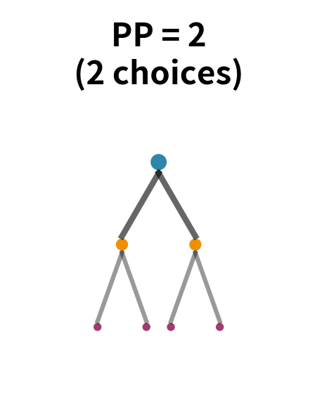
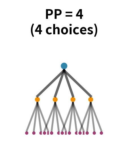
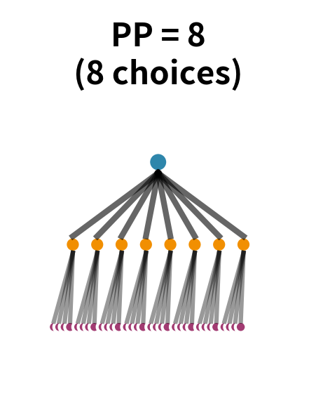
This interpretation explains why perplexity is so useful as an evaluation metric. A vocabulary of 50,000 words could theoretically produce perplexity of 50,000 (uniform distribution). A good language model achieves perplexity of 50-200 on typical text, meaning it has effectively reduced the uncertainty by orders of magnitude, from tens of thousands of possibilities to just dozens or hundreds.

Worked Example: Tracing Through the CalculationLink Copied

Let's make this concrete with a step-by-step calculation. Consider evaluating a bigram model on the sentence "the cat sat." We'll trace through exactly how perplexity emerges from the individual predictions.

Suppose our bigram model gives these probabilities:

Prediction	Probability	Interpretation
$P(\text{the} \mid \text{<s>})$	0.2	"the" is a common sentence starter
$P(\text{cat} \mid \text{the})$	0.1	"cat" is one of many words following "the"
$P(\text{sat} \mid \text{cat})$	0.05	"sat" is a plausible but not dominant verb
$P(\text{</s>} \mid \text{sat})$	0.1	sentences often end after simple verbs

The probability of the entire sequence is the product:

P(W) = 0.2 \times 0.1 \times 0.05 \times 0.1 = 0.0001

This tiny number is hard to interpret directly. But perplexity normalizes it by the sequence length. With $N = 4$ tokens:

\text{PP} = \left( \frac{1}{0.0001} \right)^{\frac{1}{4}} = (10{,}000)^{0.25} = 10

The model faces an average of 10 equally likely choices at each step. This matches our intuition from the table: some transitions are more predictable (like "the" starting a sentence with probability 0.2, equivalent to choosing among 5 options) while others are harder (like predicting "sat" after "cat" with probability 0.05, equivalent to choosing among 20 options). The geometric mean balances these out to 10.

Out[11]:

Visualization

Bar chart showing the inverse probability contribution of each word in the sequence, with a horizontal line indicating the geometric mean perplexity. — Per-word contribution to perplexity. Each word contributes differently based on how predictable it is in context. Words with lower probability (like 'sat' after 'cat') contribute more to the overall perplexity. The dashed line shows the geometric mean (final perplexity).

In[12]:

# Verify the calculation
probs = [0.2, 0.1, 0.05, 0.1]
n = len(probs)

# Method 1: Direct calculation
product = np.prod(probs)
pp_direct = (1 / product) ** (1 / n)

# Method 2: Log probability
log_probs = [np.log2(p) for p in probs]
avg_log_prob = sum(log_probs) / n
pp_log = 2 ** (-avg_log_prob)

# Verify the calculation
probs = [0.2, 0.1, 0.05, 0.1]
n = len(probs)

# Method 1: Direct calculation
product = np.prod(probs)
pp_direct = (1 / product) ** (1 / n)

# Method 2: Log probability
log_probs = [np.log2(p) for p in probs]
avg_log_prob = sum(log_probs) / n
pp_log = 2 ** (-avg_log_prob)

Out[13]:

Perplexity calculation for 'the cat sat':
--------------------------------------------------
Token probabilities: [0.2, 0.1, 0.05, 0.1]
Product of probabilities: 0.000100
Number of tokens: 4

Direct calculation: PP = (1/0.000100)^(1/4) = 10.00
Log probability method: PP = 2^(3.3219) = 10.00

Both methods give identical results, confirming our formulas are consistent. The log probability method is preferred in practice because it avoids numerical underflow. When computing products of many small probabilities, the result can become so small that floating-point arithmetic loses precision. Summing log probabilities keeps the numbers in a manageable range.

Bits Per Character and Bits Per WordLink Copied

Perplexity can be expressed in different units depending on what you're predicting.

Bits per word (BPW): This is the cross-entropy when predicting words. A perplexity of 100 corresponds to $\log_2(100) = 6.64$ bits per word.

Bits per character (BPC): When predicting characters instead of words, we use bits per character. Character-level models typically achieve 1-2 BPC on English text.

The relationship between word-level and character-level metrics depends on average word length. If the average word has $L$ characters, a rough approximation is:

\text{BPC} \approx \frac{\text{BPW}}{L + 1}

where:

$\text{BPC}$ : bits per character
$\text{BPW}$ : bits per word (cross-entropy at word level)
$L$ : average word length in characters
The $+1$ accounts for the space between words

This approximation assumes the model's uncertainty is distributed roughly uniformly across characters within words. In practice, character-level models often achieve better compression than this formula suggests because they can exploit subword regularities.

In[14]:

def perplexity_to_bits(pp):
    """Convert perplexity to bits (cross-entropy)."""
    return np.log2(pp)

def bits_to_perplexity(bits):
    """Convert bits (cross-entropy) to perplexity."""
    return 2 ** bits

# Example conversions
perplexities = [10, 50, 100, 500, 1000]

def perplexity_to_bits(pp):
    """Convert perplexity to bits (cross-entropy)."""
    return np.log2(pp)

def bits_to_perplexity(bits):
    """Convert bits (cross-entropy) to perplexity."""
    return 2 ** bits

# Example conversions
perplexities = [10, 50, 100, 500, 1000]

Out[15]:

Perplexity to Bits Conversion:
----------------------------------------
  Perplexity   Bits per word
----------------------------------------
          10            3.32
          50            5.64
         100            6.64
         500            8.97
        1000            9.97

Out[16]:

Visualization

Line plot showing the exponential relationship between bits per word and perplexity. — Relationship between perplexity and bits per word. The logarithmic relationship means that halving bits per word corresponds to squaring the perplexity. A reduction from 100 to 50 perplexity saves just 1 bit, while a reduction from 1000 to 500 also saves 1 bit.

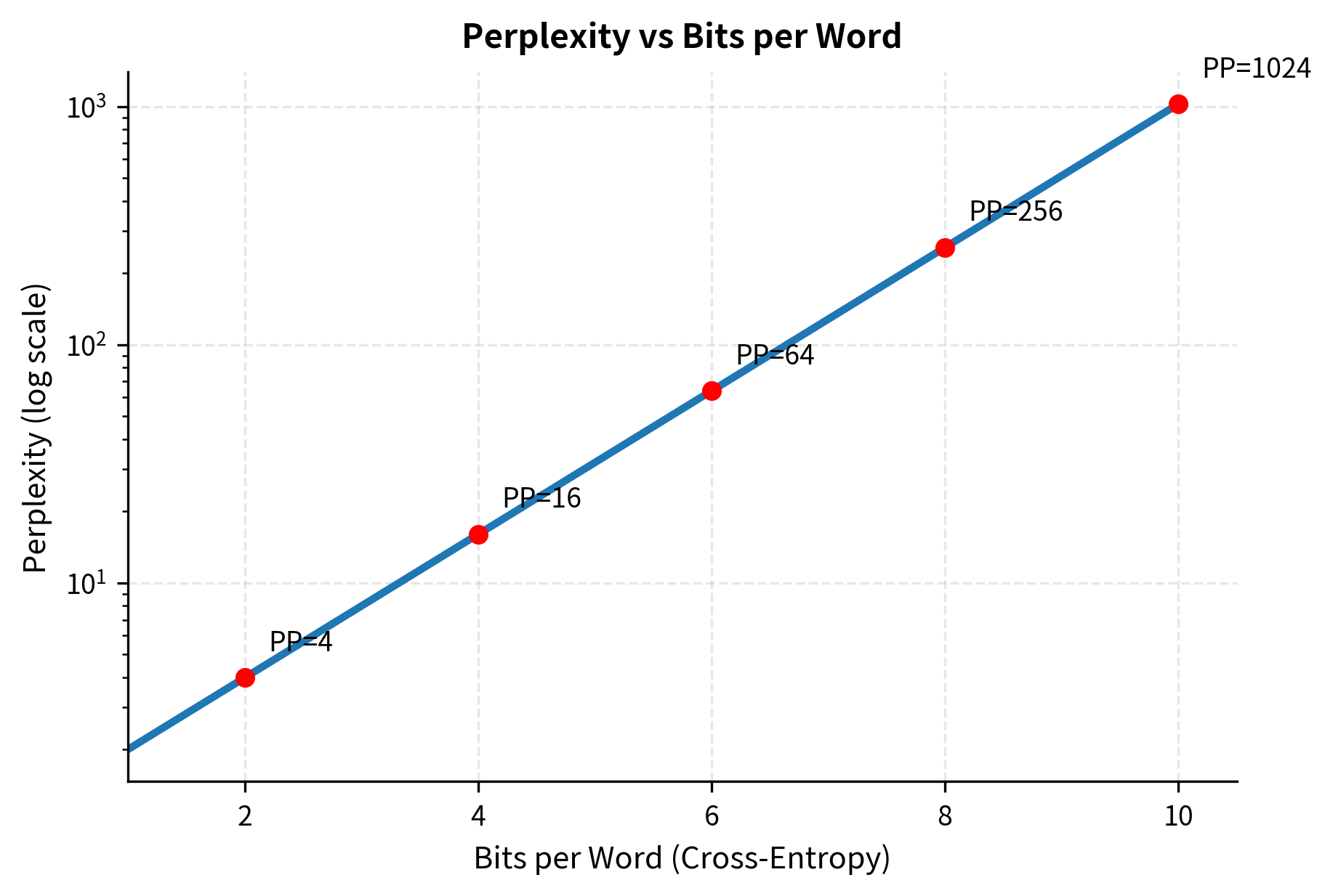
The logarithmic scale shows an important pattern: improvements in perplexity become harder as models get better. Reducing perplexity from 1000 to 500 saves the same number of bits as reducing from 100 to 50, but the latter is typically much harder to achieve.

Implementing Perplexity for N-gram ModelsLink Copied

Let's build a complete perplexity evaluation system for n-gram language models.

In[17]:

from collections import Counter, defaultdict
import math

class NgramModel:
    """N-gram language model with add-k smoothing."""
    
    def __init__(self, n=2, k=0.01):
        self.n = n
        self.k = k
        self.ngram_counts = Counter()
        self.context_counts = Counter()
        self.vocab = set()
        
    def train(self, sentences):
        """Train on a list of tokenized sentences."""
        for tokens in sentences:
            # Add start and end markers
            padded = ['<s>'] * (self.n - 1) + tokens + ['</s>']
            self.vocab.update(padded)
            
            # Count n-grams and contexts
            for i in range(len(padded) - self.n + 1):
                ngram = tuple(padded[i:i + self.n])
                context = tuple(padded[i:i + self.n - 1])
                self.ngram_counts[ngram] += 1
                self.context_counts[context] += 1
    
    def log_prob(self, word, context):
        """Return log2 P(word | context) with add-k smoothing."""
        if isinstance(context, list):
            context = tuple(context)
        
        ngram = context + (word,)
        ngram_count = self.ngram_counts.get(ngram, 0)
        context_count = self.context_counts.get(context, 0)
        
        V = len(self.vocab)
        
        # Add-k smoothing
        prob = (ngram_count + self.k) / (context_count + self.k * V)
        
        return math.log2(prob)
    
    def sentence_log_prob(self, tokens):
        """Return total log probability of a sentence."""
        padded = ['<s>'] * (self.n - 1) + tokens + ['</s>']
        
        total_log_prob = 0.0
        for i in range(self.n - 1, len(padded)):
            context = tuple(padded[i - self.n + 1:i])
            word = padded[i]
            total_log_prob += self.log_prob(word, context)
        
        return total_log_prob
    
    def perplexity(self, test_sentences):
        """Calculate perplexity on test sentences."""
        total_log_prob = 0.0
        total_words = 0
        
        for tokens in test_sentences:
            padded = ['<s>'] * (self.n - 1) + tokens + ['</s>']
            
            for i in range(self.n - 1, len(padded)):
                context = tuple(padded[i - self.n + 1:i])
                word = padded[i]
                total_log_prob += self.log_prob(word, context)
                total_words += 1
        
        avg_log_prob = total_log_prob / total_words
        return 2 ** (-avg_log_prob)

# Prepare training data
train_text = """
the cat sat on the mat
the dog sat on the rug  
the cat chased the dog
the dog chased the cat
the bird flew over the tree
the cat watched the bird
the dog watched the cat
a cat sat on a mat
a dog sat on a rug
"""

train_sentences = [line.lower().split() for line in train_text.strip().split('\n') if line.strip()]

# Train models of different orders
models = {}
for n in [1, 2, 3]:
    model = NgramModel(n=n, k=0.01)
    model.train(train_sentences)
    models[n] = model

from collections import Counter, defaultdict
import math

class NgramModel:
    """N-gram language model with add-k smoothing."""
    
    def __init__(self, n=2, k=0.01):
        self.n = n
        self.k = k
        self.ngram_counts = Counter()
        self.context_counts = Counter()
        self.vocab = set()
        
    def train(self, sentences):
        """Train on a list of tokenized sentences."""
        for tokens in sentences:
            # Add start and end markers
            padded = ['<s>'] * (self.n - 1) + tokens + ['</s>']
            self.vocab.update(padded)
            
            # Count n-grams and contexts
            for i in range(len(padded) - self.n + 1):
                ngram = tuple(padded[i:i + self.n])
                context = tuple(padded[i:i + self.n - 1])
                self.ngram_counts[ngram] += 1
                self.context_counts[context] += 1
    
    def log_prob(self, word, context):
        """Return log2 P(word | context) with add-k smoothing."""
        if isinstance(context, list):
            context = tuple(context)
        
        ngram = context + (word,)
        ngram_count = self.ngram_counts.get(ngram, 0)
        context_count = self.context_counts.get(context, 0)
        
        V = len(self.vocab)
        
        # Add-k smoothing
        prob = (ngram_count + self.k) / (context_count + self.k * V)
        
        return math.log2(prob)
    
    def sentence_log_prob(self, tokens):
        """Return total log probability of a sentence."""
        padded = ['<s>'] * (self.n - 1) + tokens + ['</s>']
        
        total_log_prob = 0.0
        for i in range(self.n - 1, len(padded)):
            context = tuple(padded[i - self.n + 1:i])
            word = padded[i]
            total_log_prob += self.log_prob(word, context)
        
        return total_log_prob
    
    def perplexity(self, test_sentences):
        """Calculate perplexity on test sentences."""
        total_log_prob = 0.0
        total_words = 0
        
        for tokens in test_sentences:
            padded = ['<s>'] * (self.n - 1) + tokens + ['</s>']
            
            for i in range(self.n - 1, len(padded)):
                context = tuple(padded[i - self.n + 1:i])
                word = padded[i]
                total_log_prob += self.log_prob(word, context)
                total_words += 1
        
        avg_log_prob = total_log_prob / total_words
        return 2 ** (-avg_log_prob)

# Prepare training data
train_text = """
the cat sat on the mat
the dog sat on the rug  
the cat chased the dog
the dog chased the cat
the bird flew over the tree
the cat watched the bird
the dog watched the cat
a cat sat on a mat
a dog sat on a rug
"""

train_sentences = [line.lower().split() for line in train_text.strip().split('\n') if line.strip()]

# Train models of different orders
models = {}
for n in [1, 2, 3]:
    model = NgramModel(n=n, k=0.01)
    model.train(train_sentences)
    models[n] = model

Out[18]:

Training corpus: 9 sentences
Vocabulary size: 16 tokens

1-gram model:
  Unique 1-grams: 15
  Unique contexts: 1
2-gram model:
  Unique 2-grams: 32
  Unique contexts: 15
3-gram model:
  Unique 3-grams: 43
  Unique contexts: 27

Now let's evaluate these models on held-out test data.

In[19]:

# Test sentences (some seen, some novel)
test_sentences = [
    "the cat sat on the mat".split(),      # Seen in training
    "the dog chased the bird".split(),     # Partially novel
    "a bird flew over the mat".split(),    # More novel combinations
    "the cat and the dog played".split(),  # Novel structure
]

# Calculate perplexity for each model
results = []
for n, model in models.items():
    pp = model.perplexity(test_sentences)
    results.append((n, pp))

# Test sentences (some seen, some novel)
test_sentences = [
    "the cat sat on the mat".split(),      # Seen in training
    "the dog chased the bird".split(),     # Partially novel
    "a bird flew over the mat".split(),    # More novel combinations
    "the cat and the dog played".split(),  # Novel structure
]

# Calculate perplexity for each model
results = []
for n, model in models.items():
    pp = model.perplexity(test_sentences)
    results.append((n, pp))

Out[20]:

Perplexity on Test Set:
----------------------------------------
       Model      Perplexity    Bits/Word
----------------------------------------
1-gram                 17.72         4.15
2-gram                  5.09         2.35
3-gram                  6.34         2.66

The results show a common pattern: higher-order models achieve lower perplexity when they have enough training data. The bigram model outperforms the unigram model because it captures local word dependencies. The trigram model may or may not improve further depending on corpus size and the specific test sentences.

Out[21]:

Visualization

Bar chart comparing perplexity values for unigram, bigram, and trigram models. — Perplexity comparison across n-gram orders. Higher-order models typically achieve lower perplexity by capturing longer-range dependencies, but gains diminish due to data sparsity. The bars show perplexity on the same test set for unigram, bigram, and trigram models.

Per-Sentence Perplexity AnalysisLink Copied

Aggregate perplexity hides important details. Let's examine how perplexity varies across individual sentences.

In[22]:

def sentence_perplexity(model, tokens):
    """Calculate perplexity for a single sentence."""
    padded = ['<s>'] * (model.n - 1) + tokens + ['</s>']
    
    total_log_prob = 0.0
    num_tokens = 0
    
    for i in range(model.n - 1, len(padded)):
        context = tuple(padded[i - model.n + 1:i])
        word = padded[i]
        total_log_prob += model.log_prob(word, context)
        num_tokens += 1
    
    avg_log_prob = total_log_prob / num_tokens
    return 2 ** (-avg_log_prob)

# Analyze each test sentence with bigram model
bigram_model = models[2]
sentence_analysis = []

for tokens in test_sentences:
    pp = sentence_perplexity(bigram_model, tokens)
    sentence_analysis.append((' '.join(tokens), pp))

def sentence_perplexity(model, tokens):
    """Calculate perplexity for a single sentence."""
    padded = ['<s>'] * (model.n - 1) + tokens + ['</s>']
    
    total_log_prob = 0.0
    num_tokens = 0
    
    for i in range(model.n - 1, len(padded)):
        context = tuple(padded[i - model.n + 1:i])
        word = padded[i]
        total_log_prob += model.log_prob(word, context)
        num_tokens += 1
    
    avg_log_prob = total_log_prob / num_tokens
    return 2 ** (-avg_log_prob)

# Analyze each test sentence with bigram model
bigram_model = models[2]
sentence_analysis = []

for tokens in test_sentences:
    pp = sentence_perplexity(bigram_model, tokens)
    sentence_analysis.append((' '.join(tokens), pp))

Out[23]:

Per-Sentence Perplexity (Bigram Model):
------------------------------------------------------------
PP =   2.32  "the cat sat on the mat"
PP =   2.69  "the dog chased the bird"
PP =   5.02  "a bird flew over the mat"
PP =  19.47  "the cat and the dog played"

Sentences that closely match training patterns have lower perplexity. Novel combinations increase perplexity because the model is less certain about them.

Out[24]:

Visualization

Horizontal bar chart showing perplexity values for different test sentences, sorted from lowest to highest. — Per-sentence perplexity shows how model confidence varies. Sentences with familiar patterns (like 'the cat sat on the mat') achieve lower perplexity than sentences with novel word combinations.

Held-Out Evaluation MethodologyLink Copied

Proper evaluation requires careful data splitting. The standard approach uses three sets:

Training set: Used to estimate model parameters (n-gram counts)
Development set (dev set): Used to tune hyperparameters (like smoothing constants)
Test set: Used only for final evaluation, never touched during development

In[25]:

def split_data(sentences, train_ratio=0.7, dev_ratio=0.15, seed=42):
    """Split data into train/dev/test sets."""
    import random
    random.seed(seed)
    
    shuffled = sentences.copy()
    random.shuffle(shuffled)
    
    n = len(shuffled)
    train_end = int(n * train_ratio)
    dev_end = int(n * (train_ratio + dev_ratio))
    
    return {
        'train': shuffled[:train_end],
        'dev': shuffled[train_end:dev_end],
        'test': shuffled[dev_end:]
    }

# Create a larger corpus for demonstration
larger_corpus = """
the quick brown fox jumps over the lazy dog
a quick brown dog runs through the green field
the lazy cat sleeps on the warm mat
a small bird sings in the tall tree
the big dog chases the small cat
a brown fox hides behind the old tree
the green field stretches to the blue horizon
a lazy dog lies in the warm sun
the tall tree provides cool shade
a quick cat catches the small mouse
the warm sun shines on the green grass
a big bird flies over the blue lake
the old tree stands in the open field
a small mouse hides in the tall grass
the blue lake reflects the clear sky
""".strip().split('\n')

corpus_sentences = [line.lower().split() for line in larger_corpus]
splits = split_data(corpus_sentences)

def split_data(sentences, train_ratio=0.7, dev_ratio=0.15, seed=42):
    """Split data into train/dev/test sets."""
    import random
    random.seed(seed)
    
    shuffled = sentences.copy()
    random.shuffle(shuffled)
    
    n = len(shuffled)
    train_end = int(n * train_ratio)
    dev_end = int(n * (train_ratio + dev_ratio))
    
    return {
        'train': shuffled[:train_end],
        'dev': shuffled[train_end:dev_end],
        'test': shuffled[dev_end:]
    }

# Create a larger corpus for demonstration
larger_corpus = """
the quick brown fox jumps over the lazy dog
a quick brown dog runs through the green field
the lazy cat sleeps on the warm mat
a small bird sings in the tall tree
the big dog chases the small cat
a brown fox hides behind the old tree
the green field stretches to the blue horizon
a lazy dog lies in the warm sun
the tall tree provides cool shade
a quick cat catches the small mouse
the warm sun shines on the green grass
a big bird flies over the blue lake
the old tree stands in the open field
a small mouse hides in the tall grass
the blue lake reflects the clear sky
""".strip().split('\n')

corpus_sentences = [line.lower().split() for line in larger_corpus]
splits = split_data(corpus_sentences)

Out[26]:

Data Split:
----------------------------------------
   train: 10 sentences
     dev: 2 sentences
    test: 3 sentences

With this split, most data goes to training, a smaller portion to development for tuning, and the rest is held out for final evaluation. The test set remains untouched until we've finalized all model choices.

Now let's use the development set to tune the smoothing parameter.

In[27]:

def tune_smoothing(train_sentences, dev_sentences, n=2):
    """Find optimal smoothing parameter k using dev set."""
    k_values = [0.001, 0.005, 0.01, 0.05, 0.1, 0.5, 1.0]
    results = []
    
    for k in k_values:
        model = NgramModel(n=n, k=k)
        model.train(train_sentences)
        pp = model.perplexity(dev_sentences)
        results.append((k, pp))
    
    return results

tuning_results = tune_smoothing(splits['train'], splits['dev'], n=2)
best_k, best_pp = min(tuning_results, key=lambda x: x[1])

def tune_smoothing(train_sentences, dev_sentences, n=2):
    """Find optimal smoothing parameter k using dev set."""
    k_values = [0.001, 0.005, 0.01, 0.05, 0.1, 0.5, 1.0]
    results = []
    
    for k in k_values:
        model = NgramModel(n=n, k=k)
        model.train(train_sentences)
        pp = model.perplexity(dev_sentences)
        results.append((k, pp))
    
    return results

tuning_results = tune_smoothing(splits['train'], splits['dev'], n=2)
best_k, best_pp = min(tuning_results, key=lambda x: x[1])

Out[28]:

Smoothing Parameter Tuning (Bigram Model):
----------------------------------------
         k  Dev Perplexity
----------------------------------------
     0.001          111.06
     0.005           59.89
     0.010           47.33
     0.050           32.07
     0.100           29.75 <-- best
     0.500           30.79
     1.000           33.06

The optimal smoothing parameter balances two competing effects. Too little smoothing (small k) assigns very low probabilities to unseen n-grams, causing high perplexity when the test set contains novel combinations. Too much smoothing (large k) flattens the probability distribution, making all words nearly equally likely regardless of context.

Out[29]:

Visualization

Line plot showing perplexity on development set as a function of smoothing parameter k, with a U-shaped curve. — Tuning the smoothing parameter k on held-out development data. Too little smoothing (small k) causes high perplexity due to very low probabilities for unseen n-grams. Too much smoothing (large k) flattens the distribution excessively. The optimal k balances these effects.

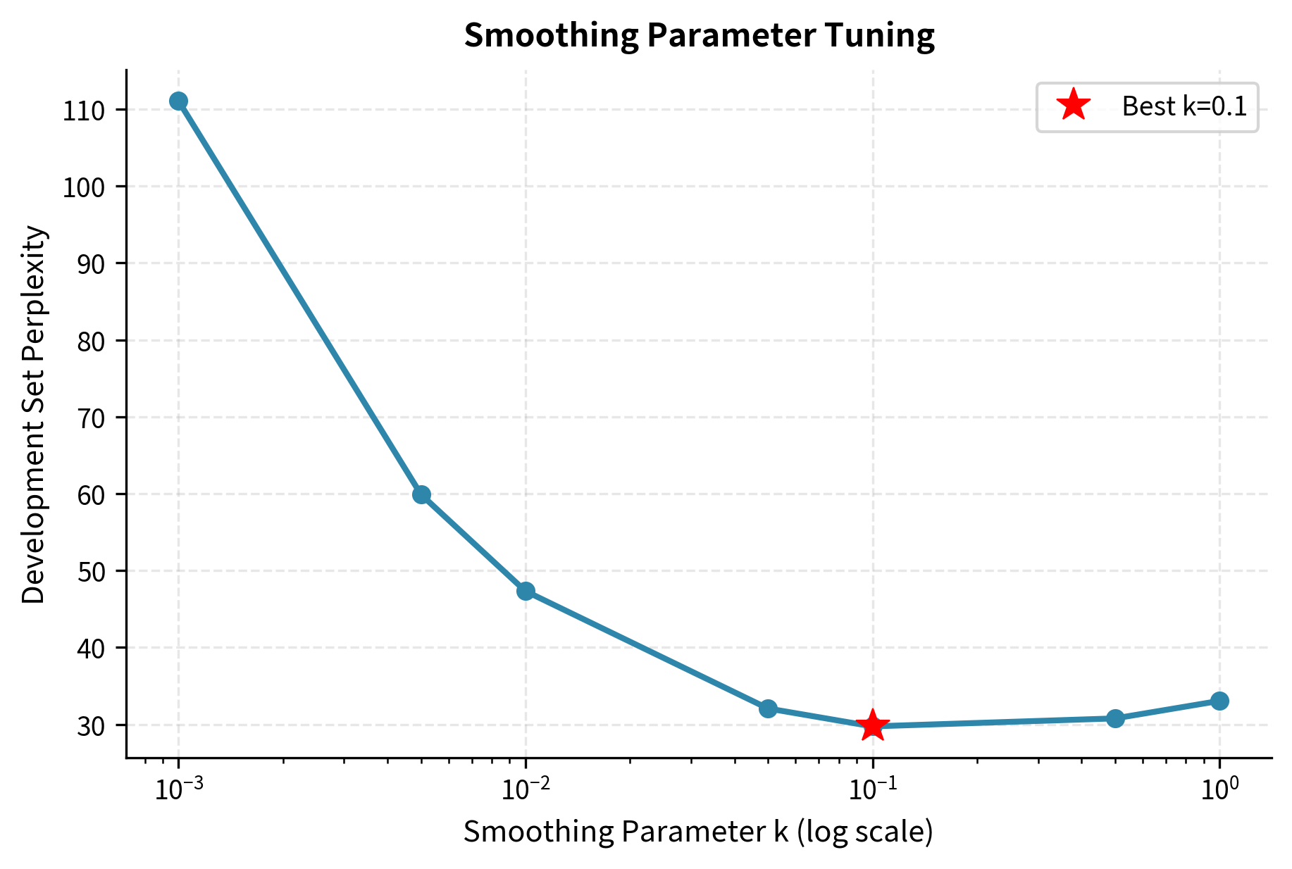
Finally, we evaluate on the test set using the tuned parameter.

In[30]:

# Train final model with best k
final_model = NgramModel(n=2, k=best_k)
final_model.train(splits['train'])

# Evaluate on test set
test_pp = final_model.perplexity(splits['test'])

# Train final model with best k
final_model = NgramModel(n=2, k=best_k)
final_model.train(splits['train'])

# Evaluate on test set
test_pp = final_model.perplexity(splits['test'])

Out[31]:

Final Evaluation:
----------------------------------------
Best smoothing parameter: k = 0.1
Development perplexity: 29.75
Test perplexity: 17.58

The test perplexity may differ from development perplexity because the test set contains different sentences. If test perplexity is much higher, it could indicate overfitting to the development set during tuning.

Comparing Models with PerplexityLink Copied

Perplexity enables fair comparison between different models, but some caveats apply.

Same Vocabulary RequirementLink Copied

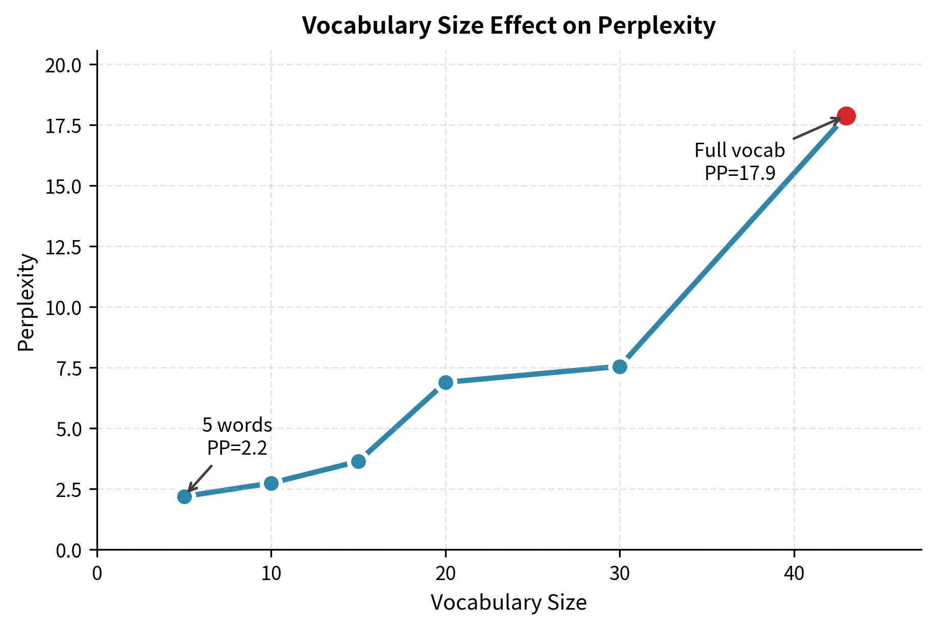
Models must use the same vocabulary for perplexity to be comparable. A model with a larger vocabulary faces a harder prediction problem because it has more choices at each step.

In[32]:

# Demonstrate vocabulary effect
def create_model_with_vocab_limit(sentences, n=2, k=0.01, max_vocab=None):
    """Create model with optional vocabulary limit."""
    model = NgramModel(n=n, k=k)
    
    if max_vocab:
        # Count word frequencies
        word_freq = Counter()
        for tokens in sentences:
            word_freq.update(tokens)
        
        # Keep only top words
        top_words = set(w for w, _ in word_freq.most_common(max_vocab))
        
        # Replace rare words with <UNK>
        filtered_sentences = []
        for tokens in sentences:
            filtered = [w if w in top_words else '<unk>' for w in tokens]
            filtered_sentences.append(filtered)
        
        model.train(filtered_sentences)
    else:
        model.train(sentences)
    
    return model

# Compare models with different vocabulary sizes
vocab_sizes = [10, 20, 50, None]  # None means full vocabulary
vocab_comparison = []

for max_v in vocab_sizes:
    model = create_model_with_vocab_limit(splits['train'], n=2, k=0.01, max_vocab=max_v)
    
    # Need to process test set with same vocabulary
    if max_v:
        word_freq = Counter()
        for tokens in splits['train']:
            word_freq.update(tokens)
        top_words = set(w for w, _ in word_freq.most_common(max_v))
        test_filtered = [[w if w in top_words else '<unk>' for w in tokens] 
                         for tokens in splits['test']]
    else:
        test_filtered = splits['test']
    
    pp = model.perplexity(test_filtered)
    vocab_comparison.append((max_v if max_v else len(model.vocab), pp))

# Demonstrate vocabulary effect
def create_model_with_vocab_limit(sentences, n=2, k=0.01, max_vocab=None):
    """Create model with optional vocabulary limit."""
    model = NgramModel(n=n, k=k)
    
    if max_vocab:
        # Count word frequencies
        word_freq = Counter()
        for tokens in sentences:
            word_freq.update(tokens)
        
        # Keep only top words
        top_words = set(w for w, _ in word_freq.most_common(max_vocab))
        
        # Replace rare words with <UNK>
        filtered_sentences = []
        for tokens in sentences:
            filtered = [w if w in top_words else '<unk>' for w in tokens]
            filtered_sentences.append(filtered)
        
        model.train(filtered_sentences)
    else:
        model.train(sentences)
    
    return model

# Compare models with different vocabulary sizes
vocab_sizes = [10, 20, 50, None]  # None means full vocabulary
vocab_comparison = []

for max_v in vocab_sizes:
    model = create_model_with_vocab_limit(splits['train'], n=2, k=0.01, max_vocab=max_v)
    
    # Need to process test set with same vocabulary
    if max_v:
        word_freq = Counter()
        for tokens in splits['train']:
            word_freq.update(tokens)
        top_words = set(w for w, _ in word_freq.most_common(max_v))
        test_filtered = [[w if w in top_words else '<unk>' for w in tokens] 
                         for tokens in splits['test']]
    else:
        test_filtered = splits['test']
    
    pp = model.perplexity(test_filtered)
    vocab_comparison.append((max_v if max_v else len(model.vocab), pp))

Out[33]:

Effect of Vocabulary Size on Perplexity:
----------------------------------------
  Vocab Size   Perplexity
----------------------------------------
          10         2.74
          20         6.89
          50        17.89
          43        17.89

Smaller vocabularies generally yield lower perplexity because the model has fewer options to choose from at each step. This illustrates why vocabulary size must be controlled when comparing models: a model with a 10-word vocabulary will always outperform one with 10,000 words on raw perplexity, even if the larger-vocabulary model is objectively better.

Out[34]:

Visualization

Line plot showing perplexity increasing as vocabulary size grows, demonstrating the relationship between vocabulary size and model perplexity. — Effect of vocabulary size on perplexity. Smaller vocabularies yield lower perplexity because the model has fewer choices at each step. This demonstrates why vocabulary size must be controlled when comparing models. Raw perplexity scores are not comparable across different vocabulary sizes.

Same Test Set RequirementLink Copied

Perplexity scores are only comparable when computed on the same test set. Different test sets may have different inherent difficulty levels.

Statistical SignificanceLink Copied

Small differences in perplexity may not be meaningful. Always consider whether improvements are statistically significant, especially when comparing on small test sets.

Perplexity vs Downstream PerformanceLink Copied

Perplexity measures how well a model predicts text, but this doesn't always translate to better performance on downstream tasks.

When Perplexity Correlates with Task PerformanceLink Copied

Perplexity tends to correlate well with tasks that directly involve predicting or generating text:

Speech recognition: Lower perplexity language models produce better transcriptions
Machine translation: Language model perplexity correlates with translation fluency
Text generation: Lower perplexity models generate more coherent text

When Perplexity Doesn't Tell the Whole StoryLink Copied

For other tasks, perplexity may be a poor predictor:

Sentiment analysis: A model might have excellent perplexity but poor sentiment predictions
Question answering: Predicting the next word well doesn't mean understanding content
Named entity recognition: Local word prediction doesn't capture entity boundaries

Out[35]:

Visualization

Bar chart showing correlation strength between perplexity and various NLP tasks, with speech recognition showing high correlation and sentiment analysis showing low correlation. — Perplexity correlates strongly with some tasks (like speech recognition) but weakly with others (like sentiment analysis). The strength of correlation depends on how closely the task relates to next-word prediction.

Limitations and CaveatsLink Copied

Out-of-Vocabulary WordsLink Copied

When the test set contains words not in the training vocabulary, standard perplexity calculation breaks. Solutions include:

Replace with <UNK>: Map unknown words to a special token
Character-level models: Avoid the OOV problem entirely
Open vocabulary: Use subword tokenization (BPE, WordPiece)

In[36]:

def perplexity_with_oov_handling(model, test_sentences, oov_token='<unk>'):
    """Calculate perplexity with OOV word handling."""
    total_log_prob = 0.0
    total_words = 0
    oov_count = 0
    
    for tokens in test_sentences:
        # Replace OOV words
        processed = []
        for w in tokens:
            if w in model.vocab:
                processed.append(w)
            else:
                processed.append(oov_token)
                oov_count += 1
        
        padded = ['<s>'] * (model.n - 1) + processed + ['</s>']
        
        for i in range(model.n - 1, len(padded)):
            context = tuple(padded[i - model.n + 1:i])
            word = padded[i]
            total_log_prob += model.log_prob(word, context)
            total_words += 1
    
    avg_log_prob = total_log_prob / total_words
    pp = 2 ** (-avg_log_prob)
    
    return pp, oov_count, total_words

# Test with sentences containing OOV words
oov_test = [
    "the elephant danced gracefully".split(),
    "a penguin swam in the ocean".split(),
]

pp, oov, total = perplexity_with_oov_handling(final_model, oov_test)

def perplexity_with_oov_handling(model, test_sentences, oov_token='<unk>'):
    """Calculate perplexity with OOV word handling."""
    total_log_prob = 0.0
    total_words = 0
    oov_count = 0
    
    for tokens in test_sentences:
        # Replace OOV words
        processed = []
        for w in tokens:
            if w in model.vocab:
                processed.append(w)
            else:
                processed.append(oov_token)
                oov_count += 1
        
        padded = ['<s>'] * (model.n - 1) + processed + ['</s>']
        
        for i in range(model.n - 1, len(padded)):
            context = tuple(padded[i - model.n + 1:i])
            word = padded[i]
            total_log_prob += model.log_prob(word, context)
            total_words += 1
    
    avg_log_prob = total_log_prob / total_words
    pp = 2 ** (-avg_log_prob)
    
    return pp, oov_count, total_words

# Test with sentences containing OOV words
oov_test = [
    "the elephant danced gracefully".split(),
    "a penguin swam in the ocean".split(),
]

pp, oov, total = perplexity_with_oov_handling(final_model, oov_test)

Out[37]:

OOV Handling Results:
----------------------------------------
Test sentences: 2
Total words: 12
OOV words: 6 (50.0%)
Perplexity (with OOV handling): 28.71

The high OOV rate reflects that these test sentences contain words like "elephant," "penguin," and "ocean" that never appeared in our training corpus. Mapping these to <unk> allows perplexity calculation to proceed, but the resulting value is less meaningful because the model treats all unknown words identically regardless of their actual likelihood.

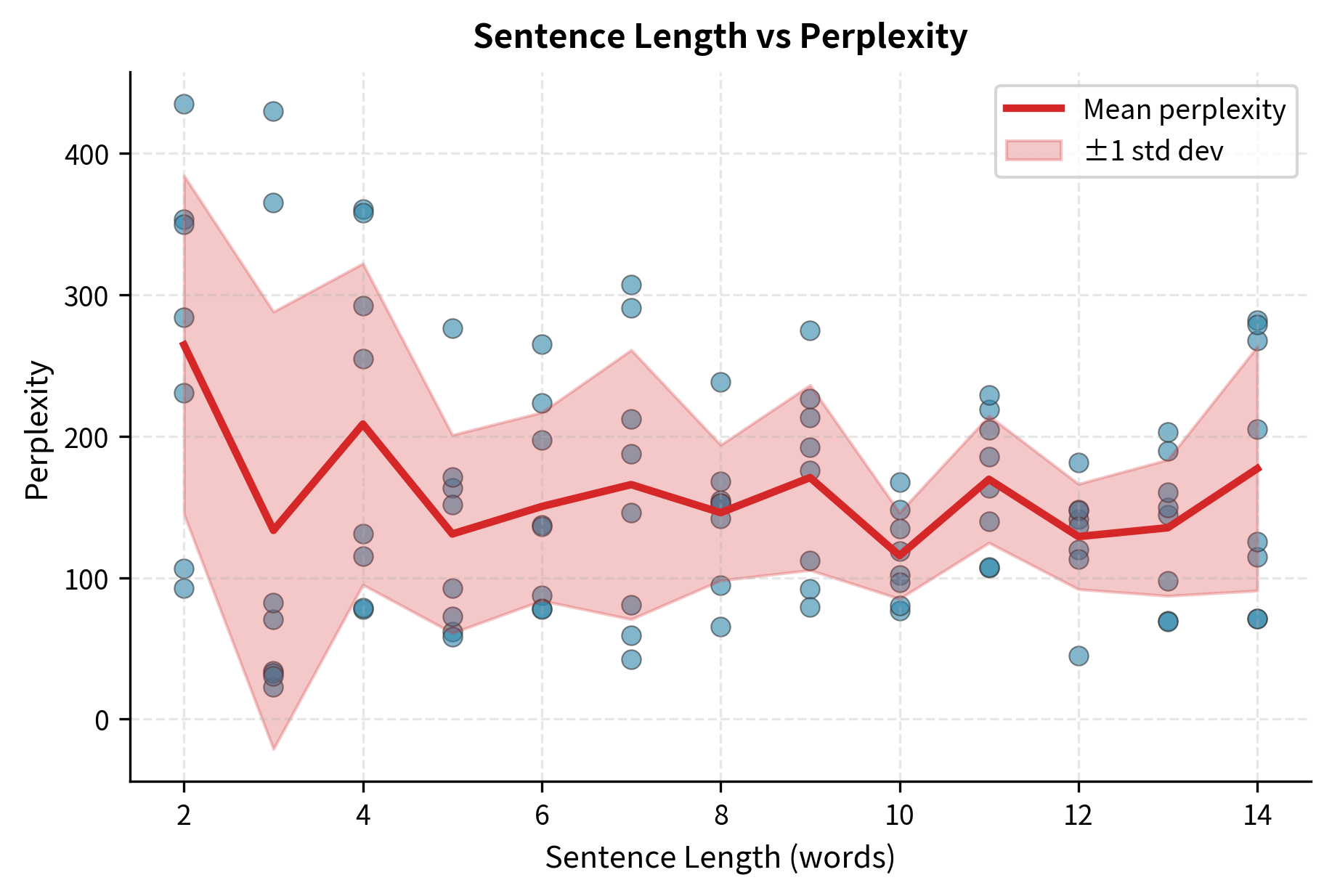
Sentence Length EffectsLink Copied

Perplexity can vary with sentence length. Very short sentences may have artificially low perplexity because they contain only common words. Very long sentences may have higher perplexity due to accumulated uncertainty.

Out[38]:

Visualization

Scatter plot showing perplexity values for sentences of different lengths, with a trend line showing how perplexity stabilizes for longer sentences. — Relationship between sentence length and perplexity. Shorter sentences tend to have more variable perplexity, while longer sentences converge toward the model's average performance. This variability in short sentences can make comparisons unreliable.

Domain MismatchLink Copied

A model trained on news text will have high perplexity on social media text, even if both are "English." This domain mismatch makes cross-domain perplexity comparisons problematic.

The Perplexity TrapLink Copied

Optimizing solely for perplexity can lead to models that are good at predicting common patterns but poor at handling rare but important cases. A model might achieve low perplexity by always predicting "the" but be useless for real applications.

Historical Context and Modern UsageLink Copied

Perplexity has been the standard language model metric since the 1980s, when it was used to evaluate early speech recognition systems. Its continued relevance speaks to its utility, but modern usage has evolved.

Classical Era (1980s-2000s)Link Copied

N-gram models were evaluated primarily by perplexity. A trigram model with Kneser-Ney smoothing might achieve perplexity around 100-200 on news text. Improvements of even 5-10% in perplexity were considered significant.

Neural Era (2010s)Link Copied

Recurrent neural networks (RNNs) and LSTMs dramatically reduced perplexity. Models achieved perplexity below 100, then below 50. Perplexity remained the primary metric for comparing architectures.

Transformer Era (2017-present)Link Copied

Transformer models pushed perplexity even lower. GPT-2 achieved perplexity around 20 on certain benchmarks. However, researchers increasingly recognize that perplexity alone doesn't capture model capabilities like reasoning, factual accuracy, or safety.

Out[39]:

Visualization

Timeline showing decreasing perplexity values from n-gram models in the 1990s to transformer models in the 2020s. — Historical progression of language model perplexity on standard benchmarks. Each architectural innovation brought significant perplexity reductions, though modern evaluation increasingly emphasizes task-specific metrics alongside perplexity.

SummaryLink Copied

Perplexity measures how well a language model predicts held-out text. It's derived from cross-entropy and can be interpreted as the effective branching factor: the average number of equally likely choices the model faces at each prediction step.

Key takeaways:

Cross-entropy measures the average bits needed to encode test data using the model's probability distribution
Perplexity equals $2^{\text{cross-entropy}}$ , converting bits to an interpretable scale
Lower perplexity means the model assigns higher probability to actual text, indicating better predictions
Branching factor interpretation: perplexity of 100 means the model is as uncertain as choosing among 100 equally likely words
Held-out evaluation prevents overfitting by testing on unseen data
Same vocabulary and test set are required for fair model comparison
Perplexity doesn't always predict task performance, especially for tasks beyond text prediction
OOV handling is essential when test data contains words not in training vocabulary

Perplexity remains the standard intrinsic evaluation metric for language models. While it doesn't capture everything important about model quality, it provides a principled, comparable measure of a model's core capability: predicting what comes next in natural language.

Key ParametersLink Copied

When computing and interpreting perplexity, these factors have the most impact:

Parameter	Typical Values	Effect
Vocabulary size	10K - 100K words	Larger vocabularies increase perplexity because the model has more choices. Always compare models with the same vocabulary.
N-gram order	2 - 5	Higher orders typically reduce perplexity but require more data. Diminishing returns beyond trigrams for most corpora.
Smoothing parameter	0.001 - 0.5	Affects perplexity through probability estimates. Tune on development data, not test data.
Test set size	10K+ words	Larger test sets give more stable perplexity estimates. Small test sets may have high variance.
OOV rate	< 5% ideal	High OOV rates make perplexity less meaningful. Consider subword tokenization for open-vocabulary evaluation.
Log base	2 or e	Using $\log_2$ gives bits; using $\ln$ gives nats. Both are valid but not directly comparable.

QuizLink Copied

Ready to test your understanding? Take this quick quiz to reinforce what you've learned about perplexity and language model evaluation.

Loading component...

Back to Language AI Handbook

Reference

BIBTEXAcademic

@misc{perplexitythestandardmetricforevaluatinglanguagemodels, author = {Michael Brenndoerfer}, title = {Perplexity: The Standard Metric for Evaluating Language Models}, year = {2025}, url = {https://mbrenndoerfer.com/writing/perplexity-language-model-evaluation-metric}, organization = {mbrenndoerfer.com}, note = {Accessed: 2025-12-08} }

APAAcademic

Michael Brenndoerfer (2025). Perplexity: The Standard Metric for Evaluating Language Models. Retrieved from https://mbrenndoerfer.com/writing/perplexity-language-model-evaluation-metric

MLAAcademic

Michael Brenndoerfer. "Perplexity: The Standard Metric for Evaluating Language Models." 2025. Web. 12/8/2025. <https://mbrenndoerfer.com/writing/perplexity-language-model-evaluation-metric>.

CHICAGOAcademic

Michael Brenndoerfer. "Perplexity: The Standard Metric for Evaluating Language Models." Accessed 12/8/2025. https://mbrenndoerfer.com/writing/perplexity-language-model-evaluation-metric.

HARVARDAcademic

Michael Brenndoerfer (2025) 'Perplexity: The Standard Metric for Evaluating Language Models'. Available at: https://mbrenndoerfer.com/writing/perplexity-language-model-evaluation-metric (Accessed: 12/8/2025).

SimpleBasic

Michael Brenndoerfer (2025). Perplexity: The Standard Metric for Evaluating Language Models. https://mbrenndoerfer.com/writing/perplexity-language-model-evaluation-metric

Direct link:

https://mbrenndoerfer.com/writing/perplexity-language-model-evaluation-metric

Part of Language AI Handbook

This article is part of the free-to-read Language AI Handbook

About the author: Michael Brenndoerfer

All opinions expressed here are my own and do not reflect the views of my employer.

Michael currently works as an Associate Director of Data Science at EQT Partners in Singapore, where he drives AI and data initiatives across private capital investments.

With over a decade of experience spanning private equity, management consulting, and software engineering, he specializes in building and scaling analytics capabilities from the ground up. He has published research in leading AI conferences and holds expertise in machine learning, natural language processing, and value creation through data.

View Full Resume Publications Contact Books

InteractivePerplexity: The Standard Metric for Evaluating Language Models

PerplexityLink Copied

The Evaluation ProblemLink Copied

Cross-Entropy: The FoundationLink Copied

Entropy: Quantifying UncertaintyLink Copied

Cross-Entropy: Measuring Model MismatchLink Copied

From Cross-Entropy to PerplexityLink Copied

The Branching Factor InterpretationLink Copied

Worked Example: Tracing Through the CalculationLink Copied

Bits Per Character and Bits Per WordLink Copied

Implementing Perplexity for N-gram ModelsLink Copied

Per-Sentence Perplexity AnalysisLink Copied

Held-Out Evaluation MethodologyLink Copied

Comparing Models with PerplexityLink Copied

Same Vocabulary RequirementLink Copied

Same Test Set RequirementLink Copied

Statistical SignificanceLink Copied

Perplexity vs Downstream PerformanceLink Copied

When Perplexity Correlates with Task PerformanceLink Copied

When Perplexity Doesn't Tell the Whole StoryLink Copied

Limitations and CaveatsLink Copied

Out-of-Vocabulary WordsLink Copied

Sentence Length EffectsLink Copied

Domain MismatchLink Copied

The Perplexity TrapLink Copied

Historical Context and Modern UsageLink Copied

Classical Era (1980s-2000s)Link Copied

Neural Era (2010s)Link Copied

Transformer Era (2017-present)Link Copied

SummaryLink Copied

Key ParametersLink Copied

QuizLink Copied

Reference

About the author: Michael Brenndoerfer

Related Content

Inverse Document Frequency: How Rare Words Reveal Document Meaning

TF-IDF: Term Frequency-Inverse Document Frequency for Text Representation

BM25: Complete Guide to the Search Algorithm Behind Elasticsearch

Stay updated